
Excel for Microsoft 365 Excel for Microsoft 365 for Mac Excel for the web Excel 2021 Excel 2021 for Mac Excel 2019 Excel 2019 for Mac Excel 2016 Excel 2016 for Mac Excel 2013 Excel 2010 Excel 2007 Excel for Mac 2011 Excel Starter 2010 More…Less
Use Excel’s DATE function when you need to take three separate values and combine them to form a date.
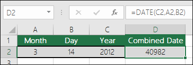
The DATE function returns the sequential serial number that represents a particular date.
Syntax: DATE(year,month,day)
The DATE function syntax has the following arguments:
-
Year Required. The value of the year argument can include one to four digits. Excel interprets the year argument according to the date system your computer is using. By default, Microsoft Excel for Windows uses the 1900 date system, which means the first date is January 1, 1900.
Tip: Use four digits for the year argument to prevent unwanted results. For example, «07» could mean «1907» or «2007.» Four digit years prevent confusion.
-
If year is between 0 (zero) and 1899 (inclusive), Excel adds that value to 1900 to calculate the year. For example, DATE(108,1,2) returns January 2, 2008 (1900+108).
-
If year is between 1900 and 9999 (inclusive), Excel uses that value as the year. For example, DATE(2008,1,2) returns January 2, 2008.
-
If year is less than 0 or is 10000 or greater, Excel returns the #NUM! error value.
-
-
Month Required. A positive or negative integer representing the month of the year from 1 to 12 (January to December).
-
If month is greater than 12, month adds that number of months to the first month in the year specified. For example, DATE(2008,14,2) returns the serial number representing February 2, 2009.
-
If month is less than 1, month subtracts the magnitude of that number of months, plus 1, from the first month in the year specified. For example, DATE(2008,-3,2) returns the serial number representing September 2, 2007.
-
-
Day Required. A positive or negative integer representing the day of the month from 1 to 31.
-
If day is greater than the number of days in the month specified, day adds that number of days to the first day in the month. For example, DATE(2008,1,35) returns the serial number representing February 4, 2008.
-
If day is less than 1, day subtracts the magnitude that number of days, plus one, from the first day of the month specified. For example, DATE(2008,1,-15) returns the serial number representing December 16, 2007.
-
Note: Excel stores dates as sequential serial numbers so that they can be used in calculations. January 1, 1900 is serial number 1, and January 1, 2008 is serial number 39448 because it is 39,447 days after January 1, 1900. You will need to change the number format (Format Cells) in order to display a proper date.
Syntax: DATE(year,month,day)
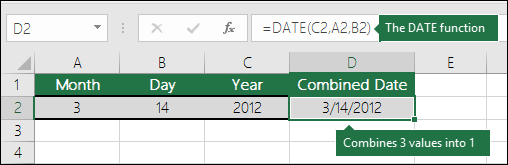
For example: =DATE(C2,A2,B2) combines the year from cell C2, the month from cell A2, and the day from cell B2 and puts them into one cell as a date. The example below shows the final result in cell D2.
Need to insert dates without a formula? No problem. You can insert the current date and time in a cell, or you can insert a date that gets updated. You can also fill data automatically in worksheet cells.
-
Right-click the cell(s) you want to change. On a Mac, Ctrl-click the cells.
-
On the Home tab click Format > Format Cells or press Ctrl+1 (Command+1 on a Mac).
-
3. Choose the Locale (location) and Date format you want.
-
For more information on formatting dates, see Format a date the way you want.

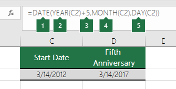
You can use the DATE function to create a date that is based on another cell’s date. For example, you can use the YEAR, MONTH, and DAY functions to create an anniversary date that’s based on another cell. Let’s say an employee’s first day at work is 10/1/2016; the DATE function can be used to establish his fifth year anniversary date:
-
The DATE function creates a date.
=DATE(YEAR(C2)+5,MONTH(C2),DAY(C2))
-
The YEAR function looks at cell C2 and extracts «2012».
-
Then, «+5» adds 5 years, and establishes «2017» as the anniversary year in cell D2.
-
The MONTH function extracts the «3» from C2. This establishes «3» as the month in cell D2.
-
The DAY function extracts «14» from C2. This establishes «14» as the day in cell D2.
If you open a file that came from another program, Excel will try to recognize dates within the data. But sometimes the dates aren’t recognizable. This is may be because the numbers don’t resemble a typical date, or because the data is formatted as text. If this is the case, you can use the DATE function to convert the information into dates. For example, in the following illustration, cell C2 contains a date that is in the format: YYYYMMDD. It is also formatted as text. To convert it into a date, the DATE function was used in conjunction with the LEFT, MID, and RIGHT functions.

-
The DATE function creates a date.
=DATE(LEFT(C2,4),MID(C2,5,2),RIGHT(C2,2))
-
The LEFT function looks at cell C2 and takes the first 4 characters from the left. This establishes “2014” as the year of the converted date in cell D2.
-
The MID function looks at cell C2. It starts at the 5th character, and then takes 2 characters to the right. This establishes “03” as the month of the converted date in cell D2. Because the formatting of D2 set to Date, the “0” isn’t included in the final result.
-
The RIGHT function looks at cell C2 and takes the first 2 characters starting from the very right and moving left. This establishes “14” as the day of the date in D2.
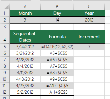
To increase or decrease a date by a certain number of days, simply add or subtract the number of days to the value or cell reference containing the date.
In the example below, cell A5 contains the date that we want to increase and decrease by 7 days (the value in C5).
See Also
Add or subtract dates
Insert the current date and time in a cell
Fill data automatically in worksheet cells
YEAR function
MONTH function
DAY function
TODAY function
DATEVALUE function
Date and time functions (reference)
All Excel functions (by category)
All Excel functions (alphabetical)
Need more help?
Содержание
- DATE function
- Format numbers as dates or times
- In this article
- Display numbers as dates or times
- Create a custom date or time format
- Tips for displaying dates or times
- Need more help?
- Excel Date and Time
- Download the Files
- Regional Settings
- Excel Date and Time 101
- In a nutshell
- Dates
- Date & Time Together
- Entering Dates & Times in Excel
- Entering Dates
- Entering Dates with Two Digit Years
- Entering Time
- Entering Dates & Time Together
- Simple Date & Time Math
- Adding/Subtracting Days from Dates
- Subtracting Dates from one another
- Adding Times to one another
- Subtracting Time from Times
- Subtracting Times from one another
- Excel Date and Time Shortcuts
- ‘Good to Know’ Stuff about Excel Date and Time
- Date Modes
- More Excel Date and Time Tips
DATE function
Use Excel’s DATE function when you need to take three separate values and combine them to form a date.
The DATE function returns the sequential serial number that represents a particular date.
The DATE function syntax has the following arguments:
Year Required. The value of the year argument can include one to four digits. Excel interprets the year argument according to the date system your computer is using. By default, Microsoft Excel for Windows uses the 1900 date system, which means the first date is January 1, 1900.
Tip: Use four digits for the year argument to prevent unwanted results. For example, «07» could mean «1907» or «2007.» Four digit years prevent confusion.
If year is between 0 (zero) and 1899 (inclusive), Excel adds that value to 1900 to calculate the year. For example, DATE(108,1,2) returns January 2, 2008 (1900+108).
If year is between 1900 and 9999 (inclusive), Excel uses that value as the year. For example, DATE(2008,1,2) returns January 2, 2008.
If year is less than 0 or is 10000 or greater, Excel returns the #NUM! error value.
Month Required. A positive or negative integer representing the month of the year from 1 to 12 (January to December).
If month is greater than 12, month adds that number of months to the first month in the year specified. For example, DATE(2008,14,2) returns the serial number representing February 2, 2009.
If month is less than 1, month subtracts the magnitude of that number of months, plus 1, from the first month in the year specified. For example, DATE(2008,-3,2) returns the serial number representing September 2, 2007.
Day Required. A positive or negative integer representing the day of the month from 1 to 31.
If day is greater than the number of days in the month specified, day adds that number of days to the first day in the month. For example, DATE(2008,1,35) returns the serial number representing February 4, 2008.
If day is less than 1, day subtracts the magnitude that number of days, plus one, from the first day of the month specified. For example, DATE(2008,1,-15) returns the serial number representing December 16, 2007.
Note: Excel stores dates as sequential serial numbers so that they can be used in calculations. January 1, 1900 is serial number 1, and January 1, 2008 is serial number 39448 because it is 39,447 days after January 1, 1900. You will need to change the number format (Format Cells) in order to display a proper date.
For example: =DATE(C2,A2,B2) combines the year from cell C2, the month from cell A2, and the day from cell B2 and puts them into one cell as a date. The example below shows the final result in cell D2.
Need to insert dates without a formula? No problem. You can insert the current date and time in a cell, or you can insert a date that gets updated. You can also fill data automatically in worksheet cells.
Right-click the cell(s) you want to change. On a Mac, Ctrl-click the cells.
On the Home tab click Format > Format Cells or press Ctrl+1 (Command+1 on a Mac).
3. Choose the Locale (location) and Date format you want.
For more information on formatting dates, see Format a date the way you want.
You can use the DATE function to create a date that is based on another cell’s date. For example, you can use the YEAR, MONTH, and DAY functions to create an anniversary date that’s based on another cell. Let’s say an employee’s first day at work is 10/1/2016; the DATE function can be used to establish his fifth year anniversary date:
The DATE function creates a date.
The YEAR function looks at cell C2 and extracts «2012».
Then, «+5» adds 5 years, and establishes «2017» as the anniversary year in cell D2.
The MONTH function extracts the «3» from C2. This establishes «3» as the month in cell D2.
The DAY function extracts «14» from C2. This establishes «14» as the day in cell D2.
If you open a file that came from another program, Excel will try to recognize dates within the data. But sometimes the dates aren’t recognizable. This is may be because the numbers don’t resemble a typical date, or because the data is formatted as text. If this is the case, you can use the DATE function to convert the information into dates. For example, in the following illustration, cell C2 contains a date that is in the format: YYYYMMDD. It is also formatted as text. To convert it into a date, the DATE function was used in conjunction with the LEFT, MID, and RIGHT functions.
The DATE function creates a date.
The LEFT function looks at cell C2 and takes the first 4 characters from the left. This establishes “2014” as the year of the converted date in cell D2.
The MID function looks at cell C2. It starts at the 5th character, and then takes 2 characters to the right. This establishes “03” as the month of the converted date in cell D2. Because the formatting of D2 set to Date, the “0” isn’t included in the final result.
The RIGHT function looks at cell C2 and takes the first 2 characters starting from the very right and moving left. This establishes “14” as the day of the date in D2.
To increase or decrease a date by a certain number of days, simply add or subtract the number of days to the value or cell reference containing the date.
In the example below, cell A5 contains the date that we want to increase and decrease by 7 days (the value in C5).
Источник
Format numbers as dates or times
When you type a date or time in a cell, it appears in a default date and time format. This default format is based on the regional date and time settings that are specified in Control Panel, and changes when you adjust those settings in Control Panel. You can display numbers in several other date and time formats, most of which are not affected by Control Panel settings.
In this article
Display numbers as dates or times
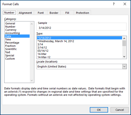
You can format dates and times as you type. For example, if you type 2/2 in a cell, Excel automatically interprets this as a date and displays 2-Feb in the cell. If this isn’t what you want—for example, if you would rather show February 2, 2009 or 2/2/09 in the cell—you can choose a different date format in the Format Cells dialog box, as explained in the following procedure. Similarly, if you type 9:30 a or 9:30 p in a cell, Excel will interpret this as a time and display 9:30 AM or 9:30 PM. Again, you can customize the way the time appears in the Format Cells dialog box.
On the Home tab, in the Number group, click the Dialog Box Launcher next to Number.

You can also press CTRL+1 to open the Format Cells dialog box.
In the Category list, click Date or Time.
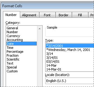
In the Type list, click the date or time format that you want to use.
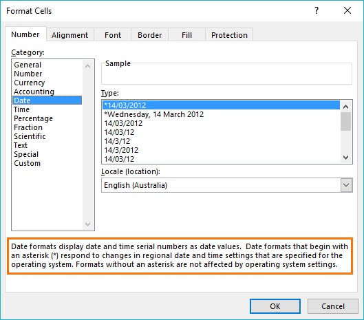
Note: Date and time formats that begin with an asterisk (*) respond to changes in regional date and time settings that are specified in Control Panel. Formats without an asterisk are not affected by Control Panel settings.
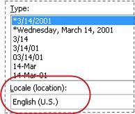
To display dates and times in the format of other languages, click the language setting that you want in the Locale (location) box.
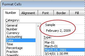
The number in the active cell of the selection on the worksheet appears in the Sample box so that you can preview the number formatting options that you selected.
Create a custom date or time format
On the Home tab, click the Dialog Box Launcher next to Number.
You can also press CTRL+1 to open the Format Cells dialog box.
In the Category box, click Date or Time, and then choose the number format that is closest in style to the one you want to create. (When creating custom number formats, it’s easier to start from an existing format than it is to start from scratch.)
In the Category box, click Custom. In the Type box, you should see the format code matching the date or time format you selected in the step 3. The built-in date or time format can’t be changed or deleted, so don’t worry about overwriting it.
In the Type box, make the necessary changes to the format. You can use any of the codes in the following tables:
Days, months, and years
Months as Jan–Dec
Months as January–December
Months as the first letter of the month
Days as Sunday–Saturday
Years as 1900–9999
If you use «m» immediately after the «h» or «hh» code or immediately before the «ss» code, Excel displays minutes instead of the month.
Hours, minutes, and seconds
Minutes as 00–59
Seconds as 00–59
Time as 4:36:03 P
Elapsed time in hours; for example, 25.02
Elapsed time in minutes; for example, 63:46
Elapsed time in seconds
Fractions of a second
AM and PM If the format contains an AM or PM, the hour is based on the 12-hour clock, where «AM» or «A» indicates times from midnight until noon and «PM» or «P» indicates times from noon until midnight. Otherwise, the hour is based on the 24-hour clock. The «m» or «mm» code must appear immediately after the «h» or «hh» code or immediately before the «ss» code; otherwise, Excel displays the month instead of minutes.
Creating custom number formats can be tricky if you haven’t done it before. For more information about how to create custom number formats, see Create or delete a custom number format.
Tips for displaying dates or times
To quickly use the default date or time format, click the cell that contains the date or time, and then press CTRL+SHIFT+# or CTRL+SHIFT+@.
If a cell displays ##### after you apply date or time formatting to it, the cell probably isn’t wide enough to display the data. To expand the column width, double-click the right boundary of the column containing the cells. This automatically resizes the column to fit the number. You can also drag the right boundary until the columns are the size you want.
When you try to undo a date or time format by selecting General in the Category list, Excel displays a number code. When you enter a date or time again, Excel displays the default date or time format. To enter a specific date or time format, such as January 2010, you can format it as text by selecting Text in the Category list.
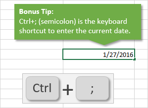
To quickly enter the current date in your worksheet, select any empty cell, and then press CTRL+; (semicolon), and then press ENTER, if necessary. To insert a date that will update to the current date each time you reopen a worksheet or recalculate a formula, type =TODAY() in an empty cell, and then press ENTER.
Need more help?
You can always ask an expert in the Excel Tech Community or get support in the Answers community.
Источник
Excel Date and Time

The objective of this post is to teach you how Excel handles date and time and provide you with all the tools you will need.
It’s designed to be read in conjunction with the accompanying Excel file, which you can download below.
Download the Files
Enter your email address below to download the comprehensive Excel workbook and PDF.
Regional Settings
When reading this post keep in mind that my regional settings format dates as dd/mm/yyyy and so the screenshots throughout this post are in this format. However, if you open the accompanying Excel file you may see some dates have switched to match your regional settings, which may be different to mine e.g. mm/dd/yyyy.
Dates and times with a format that begins with an asterisk (*) automatically update based on your PC’s regional settings. You can see an example in the Format Cells dialog box below:
Ok, let’s crack on.
Excel Date and Time 101
In a nutshell
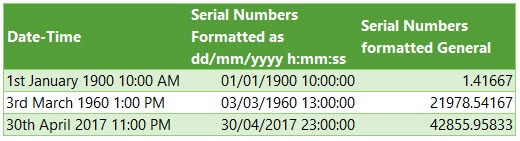
Excel stores dates and time as a number known as the date serial number, or date-time serial number.
When you look at a date in Excel it’s actually a regular number that has been formatted to look like a date. If you change the cell format to ‘General’ you’ll see the underlying date serial number.
The integer portion of the date serial number represents the day, and the decimal portion is the time. Dates start from 1st January 1900 i.e. 1/1/1900 has a date serial number of 1.
Caution! Excel dates after 28th February 1900 are actually one day out. Excel behaves as though the date 29th February 1900 existed, which it didn’t.
Microsoft intentionally included this bug in Excel so that it would remain compatible with the spreadsheet program that had the majority market share at the time; Lotus 1-2-3.
Lotus 1-2-3 was incorrectly programmed as though 1900 was a leap year. This isn’t a problem as long as all your dates are later than 1st March 1900.
Dates
Excel gives each date a numeric value starting at 1 st January 1900. 1 st January 1900 has a numeric value of 1, the 2 nd January 1900 has a numeric value of 2 and so on. These are called ‘date serial numbers’, and they enable us to do math calculations and use dates in formulas.
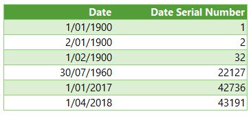
The Date Serial Number column displays the Date column values in their date serial number equivalent.
e.g. 1/1/2017 has a date serial number of 42736. i.e. 1 st January 2017 is 42,736 days since 31st December 1899.
Tip: format the date serial number column as a Date and you’ll see they look the same as the Date column values.
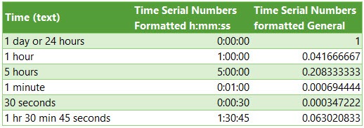
Times also use a serial number format and are represented as decimal fractions.
Hours: since 24 hours = 1 day, we can infer that 24 hours has a time serial number of 1, which can be formatted as time to display 24:00 or 12:00 AM or 0:00. Whereas 12 hours or the time 12:00 has a value of 0.50 because it is half of 24 hours or half of a day, and 1 hour is 0.41666′ because it’s 1/24 of a day.
Minutes: since 1 hour is 1/24 of a day, and 1 minute is 1/60 of an hour, we can also say that 1 minute is 1/1440 of a day, or its time serial number is 0.00069444′
Seconds: since a second is 1/60 of a minute, which is 1/60 of an hour, which is 1/24 of a day. We can also say one second is 1/86400 of a day or in time serial number form it’s 0.0000115740740740741.
Date & Time Together
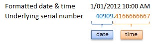
Now that we know how dates and times are stored we can put them together — ddddd.tttttt
For example, the date and time of 1 st January 2012 10:00:00 AM has a date-time serial value of 40909 . 4166666667
40909 being the serial value representing the date 1 st January 2012, and . 4166666667 being the decimal value for the time 10:00 AM and 00 seconds.
More examples below.
Entering Dates & Times in Excel
Entering Dates
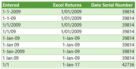
You can type in various configurations of a date and Excel will automatically recognise it as a date and upon pressing ENTER it will convert it to a date serial number and apply a date format on the cell.
For example, try typing (or even copy and paste) the following dates into an empty cell:
| 1-1-2009 |
| 1-1-09 |
| 1/1/2009 |
| 1/1/09 |
| 1-Jan-09 |
| 1-Jan 09 |
| 1-Jan-2009 |
| 1 Jan 09 |
| 1/1 |
You can see in the table above that entering numbers that look like dates and are separated by a forward slash or hyphen will be recognised as a date. Even typing in a date with the month name gets converted to a date.
However, dates separated with a period like this 1.1.2009, or with spaces between numbers like this 01 01 2009, will end up as text, not a date. Gotta have some limits!
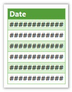
Tip: Dates that display ##### in a cell usually indicate that the column is simply not wide enough to display it.
However, if you make the cell really wide and it still displays ##### then this indicates that the date is a negative value and Excel can’t display negative dates.
Entering Dates with Two Digit Years
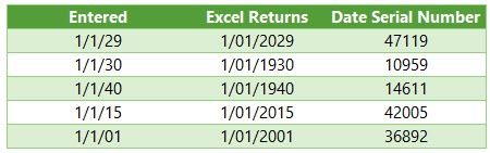
When you enter a date with two digits for the year e.g. 1/1/09, Excel has to decide if you mean 2009 or 1909.
It goes by the rule that dates with years 29 or before, are treated as 20xx and dates with the year 30 or older are treated as 19xx. See examples below.
Tip: You can enter the day and month portions of a date and Excel will insert the year based on your computer’s clock. Nice to know for data entry.
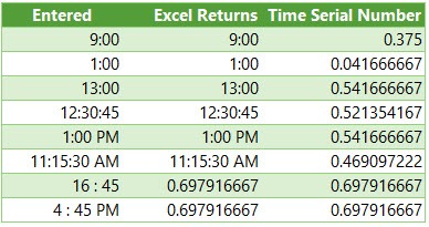
Entering Time
When you enter time you must follow a strict format of at least h:mm. i.e. the hour and minutes are separated by a colon with no spaces either side. Entering the h:mm components will result in a time formatted in military time e.g. 2:00 PM is 14:00 in military time.
If you enter a time that includes a seconds component e.g. 3:15:40, Excel will automatically format the cell in h:mm:ss.
If you want the time to be formatted with AM/PM you can simply enter a space after the time and then type AM or PM, or apply the number format to the cell later. Here are some examples:
Entering Dates & Time Together
Now that we know how to enter dates and time separately we can put them together to enter a date and time in the same cell.
You can even enter time then date and Excel will fix the order for you.
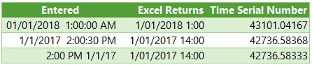
You’ll find that even if you enter AM/PM, that Excel will convert it to military time by default. You can override this with a custom number format. More on that later.
Simple Date & Time Math
Now that we understand that Excel stores dates and time as serial numbers, you’ll see how logical it is to perform math operations on these values. We’ll look at some simple examples here and tackle the more complex scenarios later when we look at Date and Time Functions.
Adding/Subtracting Days from Dates
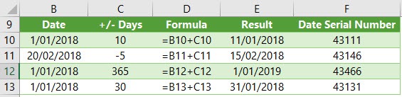
Tip: you can also add/subtract the days directly in the formula e.g. =B10+10 or =B11-5 Although, it’s better to place the values you’re adjusting by in their own cell or a named range.
Subtracting Dates from one another
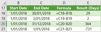
Tip: format the cell to General or Number to see the number of days between two dates.
Note: the ‘result’ is exclusive of the start day i.e. it assumes the start day is at the end of that day.
Adding Times to one another
The time being added is input as a time serial number. Notice there are no negative times in the table below. Remember we can’t display negative times. Instead we need to use the math operator to tell Excel to subtract time. See examples below.
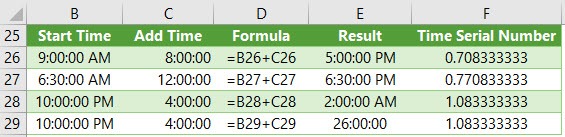
Note: Times that roll over to the next day result in a time-date serial number >= 1. Cell E28 actually contains a time-serial number of 1.08333′, but since the cell is formatted to display time formatted as h:mm:ss, only the time portion is visible.
If you want to show the cumulative time (like cell E29) then you need to surround the ‘h’ part of the time format in square brackets like so: [h]:mm:ss
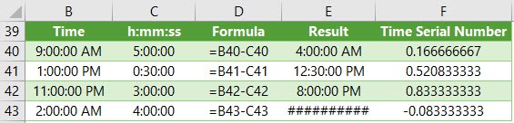
Subtracting Time from Times
Notice the last result in the table below shows ######, this is because it results in a negative time and Excel can’t display that, but notice it can return a negative time serial number. More on how to solve this later.
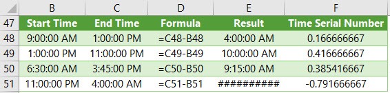
Subtracting Times from one another
Again, here the last result shows ###### because it results in a negative time.
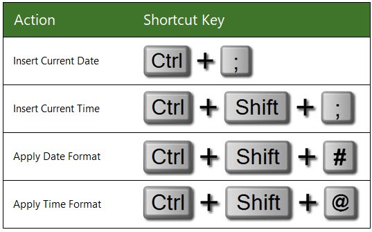
Excel Date and Time Shortcuts
‘Good to Know’ Stuff about Excel Date and Time
— Dates prior to 1st January 1900 are not recognised in Excel.
— A negative date will display in the cell as #######
— Times stored without a date effectively inherit the date 0 Jan 1900 i.e. the month is Jan and the year 1900 and the day is zero. Remember, there are no dates prior to 1/1/1900 from Excel’s perspective. This means that times stored without a date e.g. 0.50 for 12:00 PM is the equivalent of 0 Jan 1900 12:00 PM.
This is important because if you try to take 14 hours from 12 hours (without a date) you’ll get the dreaded ###### display in the cell, because negative dates and times cannot be displayed. We’ll cover workarounds for this later, but for now keep in mind that math on dates and time that result in negative date-time serial numbers cannot be formatted as a date.
Date Modes
— Excel actually has two date modes. The other mode is called 1904 Date System and is used for compatibility with Excel 2008 for Mac and earlier Mac versions. You can change the date system in the Advanced Options.
In the 1904 date system dates are calculated using 1st January 1904 as the starting point. The difference between the two date systems is 1,462 days. This means that the serial number of a date in the 1900 date system is always 1,462 days greater than the serial number of the same date in the 1904 date system. 1,462 days is equal to four years and one day (including one leap day).
Caution; the date setting you choose applies to all dates within the workbook. You can’t mix and match modes and you shouldn’t reference workbooks that use a different date system in formulas.
Bottom line; don’t use the 1904 date system unless absolutely necessary! Click here for more on date systems in Excel.
— Excel applies date number formats based on your system region settings. For example, my system is set to display dates in dd/mm/yyyy format, but if you’re in the U.S. your system is likely to format them as mm/dd/yyyy. Excel will automatically convert the format of date serial numbers to suit your system settings as long as it’s one of the default date formats and not a custom number format.
More Excel Date and Time Tips
This post is just the beginning, the next steps in mastering Excel Date and Time are below:
Tip: Avoid waiting, download the workbook and get the above topics now.
Enter your email address below to download the comprehensive Excel workbook and PDF.
Источник
Bottom line: With Valentine’s Day rapidly approaching I thought it would be good to explain how you can get a date with your Excel skills. Just kidding! 🙂 This post and video explain how the date calendar system works in Excel.
Skill level: Beginner
Dates in Excel can be just as complicated as your date for Valentine’s Day. We are going to stick with dates in Excel for this article because I’m not qualified to give any other type of dating advice. 🙂
Video Tutorial on How Dates Work in Excel
The following is a video from The Ultimate Lookup Formulas Course on how the date system works in Excel.
Watch the Video on YouTube
There are over 100 short videos just like the one above included in the Ultimate Lookup Formulas Course.
This course has been designed to help you master Excel’s most important functions and formulas in an easy step-by-step manner.
The Ultimate Lookup Formulas course is now part of our comprehensive Elevate Excel Training Program.
Click Here to Learn More About Elevate Excel
What is a Date in Excel?
I should first make it clear that I am referring to a date that is stored in a cell.
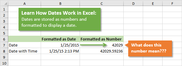
The dates in Excel are actually stored as numbers, and then formatted to display the date. The default date format for US dates is “m/d/yyyy” (1/27/2016).
The dates are referred to as serial numbers in Excel. You will see this in some of the date functions like DAY(), MONTH(), YEAR(), etc.
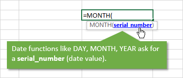
So then, what is a serial number? Well let’s start from the beginning.
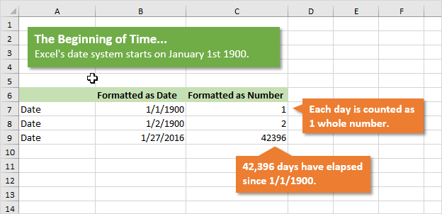
The date calendar in Excel starts on January 1st, 1900. As far as Excel is concerned this day starts the beginning of time.
Each Day is a Whole Number
Each day is represented by one whole number in Excel. Type a 1 in any cell and then format it as a date. You will get 1/1/1900. The first day of the calendar system.
Type a 2 in a cell and format it as a date. You will get 1/2/1900, or January 2nd. This means that one whole day is represented by one whole number is Excel.
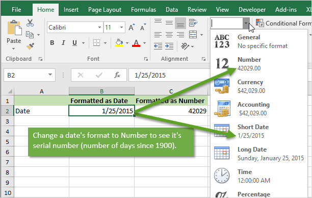
You can also take a cell that contains a date and format it as a number.
For example, this post was published on 1/27/2016. Put that number in a cell (the keyboard shortcut to enter today’s date is Ctrl+;), and then format it as a number or General.
You will see the number 42,396. This is the number of days that have elapsed since 1/1/1900.
Date Based Calculations
It is important to know that dates are stored as the number of days that have elapsed since the beginning of Excel’s calendar system (1/1/1900).
When you calculate the difference between two dates by subtraction, the result will be the number of days between the two dates.
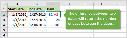
1/27/2016 – 1/1/2016 = 26 days
6/30/2016 – 1/1/2016 = 181 days
There are a lot of Date functions in Excel that can help with these calculations. Last week we learned about the DAY function for month-to-date calculations with pivot tables.
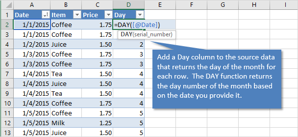
We won’t go into all the date functions here, but understanding that the serial number represents one day will give you a good foundation for working with dates.
What About Dates with Times?
Do you ever work with dates that contain time values?
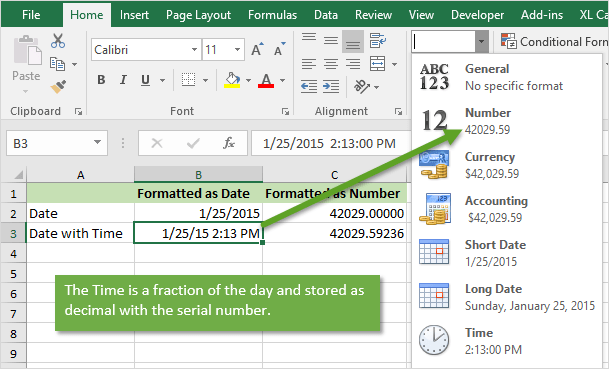
These dates are still stored as serial numbers in Excel. When you convert the date with a time to the number format, you will see a decimal number.
This decimal is a fraction of the day.
One hour in Excel is represented by the number: 1/24 = 0.04167
One minute in Excel is represented by the number: 1/(24*60) = 1/1440 = 0.000694
So 8:30 AM can be calculated as: (8 * (1/24)) + (30 * (1/1440)) = .354167
An easier way to calculate this is by typing 8:30 AM in a cell, then changing the format to Number.
So if you are running a half hour late and want to let your boss know, text him/her and say you will be there at 0.354167. 🙂
Checkout my article on 3 ways to group times in Excel for more date time based calculations.
Don’t Talk About Excel Dates with Your Date
Unless your Valentine shares a similar passion for Excel, I strongly recommend NOT sharing this information on your date.
I remember the first time I met my wife, and told her I worked in finance. The first word out of her mouth was, “BORING!”. Awe… it was love at first sight… LOL 🙂
But you should now be able to use Excel to determine how many days it has been since you last spoke to your date. That’s the only dating advice I can give.
Please leave a comment below with any questions on Excel dates. Thanks!
In Excel’s date system, dates are serial numbers beginning on January 1, 1900. January 1, 1900 is 1, January 2, 1900 is 2, and so on. More recent dates are much larger numbers. For example, January 1, 1999 is 36161, and January 1, 2010 is 40179. The table below shows a few examples of dates and their corresponding serial numbers:
| Date | Number |
|---|---|
| 1-Jan-1900 | 1 |
| 2-Jan-1900 | 2 |
| 3-Jan-1900 | 3 |
| 1-Jan-1999 | 36161 |
| 1-Jan-2010 | 40179 |
| 1-Jan-2020 | 43831 |
| 2-Jan-2020 | 43832 |
| 3-Jan-2020 | 43833 |
Because dates are just numbers, you can easily perform arithmetic on dates. For example, with the date June 1, 2020 in A1, you can add 10 days like this:
=A1+10
=43983+10
=43993
=June 11, 2020
And subtract 7 days:
=A1-7
=43983-7
=43976
=May 25, 2020
Date formats
Because Excel dates are serial numbers, you’ll sometimes see the raw numbers on a worksheet when you expect a date. To display date values in a human-readable date format, apply a number format of your choice. The easiest way to choose a date format is to use the shortcut Control + 1 to open the Format Cells dialog box:

If you can’t find the format you need in the list, you can use a custom number format to display the date.
Dates not recognized
A common problem in Excel is that dates are not correctly recognized, usually because Excel thinks the dates are text. This article explains various ways to convert text values to proper dates.
Note: to check that Excel is correctly recognizing a date, you can temporarily format the date as a number. If Excel doesn’t display the date as a number it means the date is not correctly recognized.
Create date with DATE function
You can use the DATE function to create a date with a formula using individual year, month, and day components. For example, the following formula creates the date «March 10, 2020»:
=DATE(2020,3,10)
Dates with Times
Dates can include times as well, since time values are just fractions of a 24-hour day. To create a date with a time using a formula, you can use the DATE and TIME function together. For example, the following formula creates the date value for «March 10, 2020 9:00 PM»:
=DATE(2020,3,10)+TIME(21,0,0)
Note: Excel will only handle dates after 1/1/1900.
The objective of this post is to teach you how Excel handles date and time and provide you with all the tools you will need.
It’s designed to be read in conjunction with the accompanying Excel file, which you can download below.
Download the Files
Enter your email address below to download the comprehensive Excel workbook and PDF.
By submitting your email address you agree that we can email you our Excel newsletter.
Regional Settings
When reading this post keep in mind that my regional settings format dates as dd/mm/yyyy and so the screenshots throughout this post are in this format. However, if you open the accompanying Excel file you may see some dates have switched to match your regional settings, which may be different to mine e.g. mm/dd/yyyy.
Dates and times with a format that begins with an asterisk (*) automatically update based on your PC’s regional settings. You can see an example in the Format Cells dialog box below:
Ok, let’s crack on.
Excel Date and Time 101
Excel stores dates and time as a number known as the date serial number, or date-time serial number.
When you look at a date in Excel it’s actually a regular number that has been formatted to look like a date. If you change the cell format to ‘General’ you’ll see the underlying date serial number.
The integer portion of the date serial number represents the day, and the decimal portion is the time. Dates start from 1st January 1900 i.e. 1/1/1900 has a date serial number of 1.
Caution! Excel dates after 28th February 1900 are actually one day out. Excel behaves as though the date 29th February 1900 existed, which it didn’t.
Microsoft intentionally included this bug in Excel so that it would remain compatible with the spreadsheet program that had the majority market share at the time; Lotus 1-2-3.
Lotus 1-2-3 was incorrectly programmed as though 1900 was a leap year. This isn’t a problem as long as all your dates are later than 1st March 1900.
Excel gives each date a numeric value starting at 1st January 1900. 1st January 1900 has a numeric value of 1, the 2nd January 1900 has a numeric value of 2 and so on. These are called ‘date serial numbers’, and they enable us to do math calculations and use dates in formulas.
The Date Serial Number column displays the Date column values in their date serial number equivalent.
e.g. 1/1/2017 has a date serial number of 42736. i.e. 1st January 2017 is 42,736 days since 31st December 1899.
Tip: format the date serial number column as a Date and you’ll see they look the same as the Date column values.
Time
Times also use a serial number format and are represented as decimal fractions.
Hours: since 24 hours = 1 day, we can infer that 24 hours has a time serial number of 1, which can be formatted as time to display 24:00 or 12:00 AM or 0:00. Whereas 12 hours or the time 12:00 has a value of 0.50 because it is half of 24 hours or half of a day, and 1 hour is 0.41666′ because it’s 1/24 of a day.
Minutes: since 1 hour is 1/24 of a day, and 1 minute is 1/60 of an hour, we can also say that 1 minute is 1/1440 of a day, or its time serial number is 0.00069444′
Seconds: since a second is 1/60 of a minute, which is 1/60 of an hour, which is 1/24 of a day. We can also say one second is 1/86400 of a day or in time serial number form it’s 0.0000115740740740741…
Date & Time Together
Now that we know how dates and times are stored we can put them together — ddddd.tttttt
For example, the date and time of 1st January 2012 10:00:00 AM has a date-time serial value of 40909.4166666667
40909 being the serial value representing the date 1st January 2012, and .4166666667 being the decimal value for the time 10:00 AM and 00 seconds.
More examples below.
Entering Dates & Times in Excel
Entering Dates
You can type in various configurations of a date and Excel will automatically recognise it as a date and upon pressing ENTER it will convert it to a date serial number and apply a date format on the cell.
For example, try typing (or even copy and paste) the following dates into an empty cell:
| 1-1-2009 |
| 1-1-09 |
| 1/1/2009 |
| 1/1/09 |
| 1-Jan-09 |
| 1-Jan 09 |
| 1-Jan-2009 |
| 1 Jan 09 |
| 1/1 |
You can see in the table above that entering numbers that look like dates and are separated by a forward slash or hyphen will be recognised as a date. Even typing in a date with the month name gets converted to a date.
However, dates separated with a period like this 1.1.2009, or with spaces between numbers like this 01 01 2009, will end up as text, not a date. Gotta have some limits!
Tip: Dates that display ##### in a cell usually indicate that the column is simply not wide enough to display it.
However, if you make the cell really wide and it still displays ##### then this indicates that the date is a negative value and Excel can’t display negative dates.
Entering Dates with Two Digit Years
When you enter a date with two digits for the year e.g. 1/1/09, Excel has to decide if you mean 2009 or 1909.
It goes by the rule that dates with years 29 or before, are treated as 20xx and dates with the year 30 or older are treated as 19xx. See examples below.
Tip: You can enter the day and month portions of a date and Excel will insert the year based on your computer’s clock. Nice to know for data entry.
Entering Time
When you enter time you must follow a strict format of at least h:mm. i.e. the hour and minutes are separated by a colon with no spaces either side. Entering the h:mm components will result in a time formatted in military time e.g. 2:00 PM is 14:00 in military time.
If you enter a time that includes a seconds component e.g. 3:15:40, Excel will automatically format the cell in h:mm:ss.
If you want the time to be formatted with AM/PM you can simply enter a space after the time and then type AM or PM, or apply the number format to the cell later. Here are some examples:
Entering Dates & Time Together
Now that we know how to enter dates and time separately we can put them together to enter a date and time in the same cell.
You can even enter time then date and Excel will fix the order for you.
You’ll find that even if you enter AM/PM, that Excel will convert it to military time by default. You can override this with a custom number format. More on that later.
Simple Date & Time Math
Now that we understand that Excel stores dates and time as serial numbers, you’ll see how logical it is to perform math operations on these values. We’ll look at some simple examples here and tackle the more complex scenarios later when we look at Date and Time Functions.
Adding/Subtracting Days from Dates
Tip: you can also add/subtract the days directly in the formula e.g. =B10+10 or =B11-5 Although, it’s better to place the values you’re adjusting by in their own cell or a named range.
Subtracting Dates from one another
Tip: format the cell to General or Number to see the number of days between two dates.
Note: the ‘result’ is exclusive of the start day i.e. it assumes the start day is at the end of that day.
Adding Times to one another
The time being added is input as a time serial number. Notice there are no negative times in the table below. Remember we can’t display negative times. Instead we need to use the math operator to tell Excel to subtract time. See examples below.
Note: Times that roll over to the next day result in a time-date serial number >= 1. Cell E28 actually contains a time-serial number of 1.08333′, but since the cell is formatted to display time formatted as h:mm:ss, only the time portion is visible.
If you want to show the cumulative time (like cell E29) then you need to surround the ‘h’ part of the time format in square brackets like so: [h]:mm:ss
Subtracting Time from Times
Notice the last result in the table below shows ######, this is because it results in a negative time and Excel can’t display that, but notice it can return a negative time serial number. More on how to solve this later.
Subtracting Times from one another
Again, here the last result shows ###### because it results in a negative time.
Excel Date and Time Shortcuts
‘Good to Know’ Stuff about Excel Date and Time
— Dates prior to 1st January 1900 are not recognised in Excel.
— A negative date will display in the cell as #######
— Times stored without a date effectively inherit the date 0 Jan 1900 i.e. the month is Jan and the year 1900 and the day is zero. Remember, there are no dates prior to 1/1/1900 from Excel’s perspective. This means that times stored without a date e.g. 0.50 for 12:00 PM is the equivalent of 0 Jan 1900 12:00 PM.
This is important because if you try to take 14 hours from 12 hours (without a date) you’ll get the dreaded ###### display in the cell, because negative dates and times cannot be displayed. We’ll cover workarounds for this later, but for now keep in mind that math on dates and time that result in negative date-time serial numbers cannot be formatted as a date.
Date Modes
— Excel actually has two date modes. The other mode is called 1904 Date System and is used for compatibility with Excel 2008 for Mac and earlier Mac versions. You can change the date system in the Advanced Options.
In the 1904 date system dates are calculated using 1st January 1904 as the starting point. The difference between the two date systems is 1,462 days. This means that the serial number of a date in the 1900 date system is always 1,462 days greater than the serial number of the same date in the 1904 date system. 1,462 days is equal to four years and one day (including one leap day).
Caution; the date setting you choose applies to all dates within the workbook. You can’t mix and match modes and you shouldn’t reference workbooks that use a different date system in formulas.
Bottom line; don’t use the 1904 date system unless absolutely necessary! Click here for more on date systems in Excel.
— Excel applies date number formats based on your system region settings. For example, my system is set to display dates in dd/mm/yyyy format, but if you’re in the U.S. your system is likely to format them as mm/dd/yyyy. Excel will automatically convert the format of date serial numbers to suit your system settings as long as it’s one of the default date formats and not a custom number format.
More Excel Date and Time Tips
This post is just the beginning, the next steps in mastering Excel Date and Time are below:
- Every Excel Date and Time Function explained
- Formatting Date and Time in Excel
- Common Date and Time Calculations
Tip: Avoid waiting, download the workbook and get the above topics now.
Enter your email address below to download the comprehensive Excel workbook and PDF.
By submitting your email address you agree that we can email you our Excel newsletter.