
Excel for Microsoft 365 Excel for Microsoft 365 for Mac Excel for the web Excel 2021 Excel 2021 for Mac Excel 2019 Excel 2019 for Mac Excel 2016 Excel 2016 for Mac Excel 2013 Excel 2010 Excel 2007 Excel for Mac 2011 Excel Starter 2010 More…Less
This article describes the formula syntax and usage of the AVERAGE function in Microsoft Excel.
Description
Returns the average (arithmetic mean) of the arguments. For example, if the range A1:A20 contains numbers, the formula =AVERAGE(A1:A20) returns the average of those numbers.
Syntax
AVERAGE(number1, [number2], …)
The AVERAGE function syntax has the following arguments:
-
Number1 Required. The first number, cell reference, or range for which you want the average.
-
Number2, … Optional. Additional numbers, cell references or ranges for which you want the average, up to a maximum of 255.
Remarks
-
Arguments can either be numbers or names, ranges, or cell references that contain numbers.
-
Logical values and text representations of numbers that you type directly into the list of arguments are not counted.
-
If a range or cell reference argument contains text, logical values, or empty cells, those values are ignored; however, cells with the value zero are included.
-
Arguments that are error values or text that cannot be translated into numbers cause errors.
-
If you want to include logical values and text representations of numbers in a reference as part of the calculation, use the AVERAGEA function.
-
If you want to calculate the average of only the values that meet certain criteria, use the AVERAGEIF function or the AVERAGEIFS function.
Note: The AVERAGE function measures central tendency, which is the location of the center of a group of numbers in a statistical distribution. The three most common measures of central tendency are:
-
Average, which is the arithmetic mean, and is calculated by adding a group of numbers and then dividing by the count of those numbers. For example, the average of 2, 3, 3, 5, 7, and 10 is 30 divided by 6, which is 5.
-
Median, which is the middle number of a group of numbers; that is, half the numbers have values that are greater than the median, and half the numbers have values that are less than the median. For example, the median of 2, 3, 3, 5, 7, and 10 is 4.
-
Mode, which is the most frequently occurring number in a group of numbers. For example, the mode of 2, 3, 3, 5, 7, and 10 is 3.
For a symmetrical distribution of a group of numbers, these three measures of central tendency are all the same. For a skewed distribution of a group of numbers, they can be different.
Tip: When you average cells, keep in mind the difference between empty cells and those containing the value zero, especially if you have cleared the Show a zero in cells that have a zero value check box in the Excel Options dialog box in the Excel desktop application. When this option is selected, empty cells are not counted, but zero values are.
To locate the Show a zero in cells that have a zero value check box:
-
On the File tab, click Options, and then, in the Advanced category, look under Display options for this worksheet.
Example
Copy the example data in the following table, and paste it in cell A1 of a new Excel worksheet. For formulas to show results, select them, press F2, and then press Enter. If you need to, you can adjust the column widths to see all the data.
|
Data |
||
|
10 |
15 |
32 |
|
7 |
||
|
9 |
||
|
27 |
||
|
2 |
||
|
Formula |
Description |
Result |
|
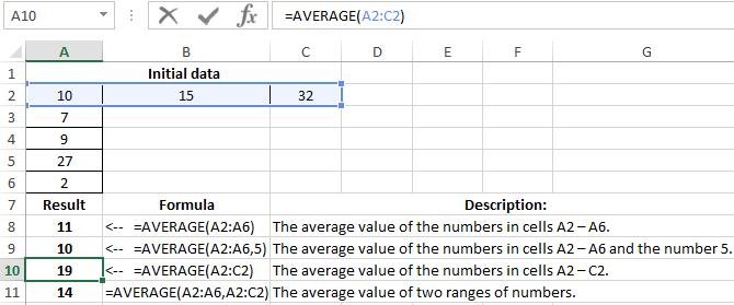
=AVERAGE(A2:A6) |
Average of the numbers in cells A2 through A6. |
11 |
|
=AVERAGE(A2:A6, 5) |
Average of the numbers in cells A2 through A6 and the number 5. |
10 |
|
=AVERAGE(A2:C2) |
Average of the numbers in cells A2 through C2. |
19 |
Need more help?
Want more options?
Explore subscription benefits, browse training courses, learn how to secure your device, and more.
Communities help you ask and answer questions, give feedback, and hear from experts with rich knowledge.
The AVERAGE function calculates the average of numbers provided as arguments. To calculate the average, Excel sums all numeric values and divides by the count of numeric values.
AVERAGE takes multiple arguments in the form number1, number2, number3, etc. up to 255 total. Arguments can include numbers, cell references, ranges, arrays, and constants. Empty cells, and cells that contain text or logical values are ignored. However, zero (0) values are included. You can ignore zero (0) values with the AVERAGEIFS function, as explained below.
The AVERAGE function will ignore logical values and numbers entered as text. If you need to include these values in the average, see the AVERAGEA function.
If the values given to AVERAGE contain errors, AVERAGE returns an error. You can use the AGGREGATE function to ignore errors.
Basic usage
A typical way to use the AVERAGE function is to provide a range, as seen below. The formula in F3, copied down, is:
=AVERAGE(C3:E3)

At each new row, AVERAGE calculates an average of the quiz scores for each person.
Blank cells
The AVERAGE function automatically ignores blank cells. In the screen below, notice cell C4 is empty, and AVERAGE simply ignores it and computes an average with B4 and D4 only:

However, note the zero (0) value in C5 is included in the average, since it is a valid numeric value. To exclude zero values, use AVERAGEIF or AVERAGEIFS instead. In the example below, AVERAGEIF is used to exclude zero values. Like the AVERAGE function, AVERAGEIF automatically excludes empty cells.
=AVERAGEIF(B3:D3,">0") // exclude zero

Mixed arguments
The numbers provided to AVERAGE can be a mix of references and constants:

=AVERAGE(A1,A2,4) // returns 3
Average with criteria
To calculate an average with criteria, use AVERAGEIF or AVERAGEIFS. In the example below, AVERAGEIFS is used to calculate the average score for Red and Blue groups:

=AVERAGEIFS(C5:C14,D5:D14,"red") // red average
=AVERAGEIFS(C5:C14,D5:D14,"blue") // blue average
The AVERAGEIFS function can also apply multiple criteria.
Average top 3
By combining the AVERAGE function with the LARGE function, you can calculate an average of top n values. In the example below, the formula in column I computes an average of the top 3 quiz scores in each row:

Detailed explanation here.
Weighted average
To calculate a weighted average, you’ll want to use the SUMPRODUCT function, as shown below:

Read a complete explanation here.
Average without #DIV/0!
The average function automatically ignores empty cells in a set of data. However, if the range contains no numeric values, AVERAGE will return a #DIV/0! error. To avoid this problem, you can check the count of values with the COUNT function and the IF function like this:
=IF(COUNT(range)>0,AVERAGE(range),"") // check count first
When the count of numeric values is zero, IF returns an empty string («»). When the count is greater than zero, AVERAGE returns the average. This example explains this idea in more detail.
Manual average
To calculate the average, AVERAGE sums all numeric values and divides by the count of numeric values. This behavior can be replicated with the SUM and COUNT functions manually like this:
=SUM(range)/COUNT(range) // manual average calculation
Notes
- AVERAGE automatically ignores empty cells and cells with text values.
- AVERAGE includes zero values. Use AVERAGEIF or AVERAGEIFS to ignore zero values.
- Arguments can be supplied as constants, ranges, named ranges, or cell references.
- AVERAGE can handle up to 255 total arguments.
- To see a quick average without a formula, you can use the status bar.
The AVERAGE function in Excel calculates the arithmetic mean of the supplied values. Such values can be numbers, percentages or times. In the mean (or average), the sum of all the items is divided by the number of items on the list. Apart from numbers, an average of Boolean values (true and false) can also be found if they are typed directly in the AVERAGE formula.
For example, the formula “=AVERAGE(10,24,35,true,false)” returns 14. The “true” and “false” values are counted as 1 and 0 respectively. So, the mean is (10+24+35+1+0)/5=14.
The purpose of using the AVERAGE function in Excel is to calculate the center or meanArithmetic mean denotes the average of all the observations of a data series. It is the aggregate of all the values in a data set divided by the total count of the observations.read more of a list. A mean includes every value of the list in the calculation. As a result, it is impacted by the extreme values or outliers (very small or very big values) of a list. The AVERAGE function is categorized as a Statistical function of Excel.
Table of contents
- What is Average Function in Excel?
- Syntax of the AVERAGE Function of Excel
- Features of the AVERAGE function of Excel
- How to Use the AVERAGE Function of Excel?
- Example #1–Average in Five Different Cases
- Example #2–Average by Supplying a Horizontal Range Reference
- Example #3–Average and Maximum Average Revenue by AVERAGE, LOOKUP, and MAX Functions
- Example #4–Average of Top Four Scores by AVERAGE and LARGE Functions
- Example #5–Average of Last Three Numbers by AVERAGE, LOOKUP, LARGE, IF, ISNUMBER, and ROW Functions
- Frequently Asked Questions
- AVERAGE Function in Excel Video
- Recommended Articles
Syntax of the AVERAGE Function of Excel
The syntax of the AVERAGE function of Excel is shown in the following image:

The AVERAGE function of Excel accepts the following arguments:
- Number 1: This is the first number for which the average is to be calculated.
- Number 2, number 3,…number n: These are the subsequent numbers for which the average is to be calculated.
The numbers can be supplied as direct numbers, named ranges or cell referencesCell reference in excel is referring the other cells to a cell to use its values or properties. For instance, if we have data in cell A2 and want to use that in cell A1, use =A2 in cell A1, and this will copy the A2 value in A1.read more containing numeric values. The first number is required, while the subsequent numbers are optional. However, for computing an average, at least two numbers are needed.
Note: The output of other Excel functions can also serve as an input to the AVERAGE function. However, such an output must necessarily be a numeric value.
Features of the AVERAGE function of Excel
The features of the AVERAGE function of Excel are listed as follows:
- It can be supplied with a maximum of 255 arguments in a single formula.
- It ignores the logical values (or Boolean values) if they have been supplied as cell references. However, logical values entered directly in the formula are counted by the function.
- It counts those cell references that contain numbers formatted as text.
- It treats the text strings as follows:
- If the entire range reference consists of a few numbers and some text strings, the average of only the numbers is returned. In this case, the text strings supplied in the range reference are ignored by the function.
- If the entire range reference consists of text strings, the “#DIV/0!” error is returned by the function.
- If text strings are entered directly in the formula, it returns the “#VALUE!” error.
- It excludes the empty cells from the count. But, the cells containing the number zero are counted.
- It returns an error if the arguments supplied are error values.
Note: To include the zero values and exclude the empty cells from the count, follow the listed steps:
- Click “options” from the File tab. The “Excel options” window opens.
- Click “advanced” displayed on the left side.
- Under “display options for this worksheet,” select the checkbox of “show a zero in cells that have zero value.”
The zero values of cells will be displayed and included in the count by the AVERAGE function of Excel. Deselecting the checkbox in point “c” will hide the zero values and display empty cells in their place.
How to Use the AVERAGE Function of Excel?
The AVERAGE function is one of the most used functions of Excel. It is frequently used in the financial sectorThe financial sector refers to businesses, firms, banks, and institutions providing financial services and supporting the economy. It encompasses several industries, including banking and investment, consumer finance, mortgage, money markets, real estate, insurance, retail, etc.read more to calculate the average revenue generated by an organization in a specific time period. It is also used to do financial modelingFinancial modeling refers to the use of excel-based models to reflect a company’s projected financial performance. Such models represent the financial situation by taking into account risks and future assumptions, which are critical for making significant decisions in the future, such as raising capital or valuing a business, and interpreting their impact.read more and analyze datasets.
Let us consider a few examples to understand the working of the AVERAGE function of Excel.
You can download this AVERAGE Function Excel Template here – AVERAGE Function Excel Template
Example #1–Average in Five Different Cases
The following image shows a list of numbers in the range B3:B7. Use the AVERAGE function of Excel to perform the tasks stated within the following cases:
- Case 1: Calculate the average by supplying a vertical range reference.
- Case 2: Calculate the average by supplying the numbers directly to the function.
- Case 3: Calculate the average by supplying the numbers in words. Enclose the text strings within double quotation marks.
- Case 4: Calculate the average by supplying the references of cells containing the number names.
- Case 5: Calculate the average by supplying the numbers directly within double quotation marks.
Write a conclusion for each case.

Case 1: Supply a vertical range reference
The steps are listed as follows:
Step 1: Enter the following formula in cell C3.
“=AVERAGE(B3:B7)”
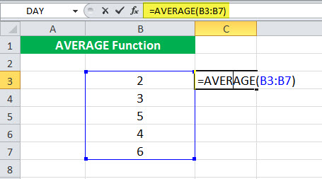
Step 2: Press the “Enter” key. The output in cell C3 is 4. So, the mean of the given numbers is 4. This is shown within a red box in the following image.

Conclusion: For calculating the average, the numbers can be supplied as a range reference. It is also possible to supply cell referencesCell reference in excel is referring the other cells to a cell to use its values or properties. For instance, if we have data in cell A2 and want to use that in cell A1, use =A2 in cell A1, and this will copy the A2 value in A1.read more of non-adjacent cells.
Simply select the cell or range in order to supply it to the AVERAGE function. Further, ensure that the non-contiguous cells or ranges are separated by commas.
Case 2: Supply the numbers directly to the AVERAGE function
The steps are listed as follows:
Step 1: Enter the following formula in cell C4.
“=AVERAGE(2,3,5,4,6)”

Step 2: Press the “Enter” key. The output is shown in cell C4 of the following image. Hence, the mean is again 4.

Conclusion: It is possible to supply the numbers directly to the AVERAGE function. One need not enclose such numbers within double quotation marks.
However, when there are too many numbers in the list, it becomes difficult to enter them directly. In such cases, it is easier to supply cell references.
Case 3: Supply the numbers in words
The steps are listed as follows:
Step 1: Enter the following formula in cell C5.
“=AVERAGE(“Two”,”Three”,”Five”,”Four”,”Six”)”

Step 2: Press the “Enter” key. The output in cell C5 is the “#VALUE!” error. This is shown in the following image.

Conclusion: When the number names are supplied directly to the AVERAGE function, it returns the“#VALUE!” error. This implies that the AVERAGE function does not work with text strings, even if such strings are enclosed within double quotation marks.
Case 4: Supply the references to cells containing the number names
The steps are listed as follows:
Step 1: Write the names of the numbers in the range A3:A7. Next, enter the following formula in cell C6.
“=AVERAGE(A3:A7)”

Step 2: Press the “Enter” key. The output in cell C6 is the “#DIV/0!” error. This is shown in the following image.

Conclusion: If number names are supplied as cell references, the AVERAGE function returns the “#DIV/0!” error. This implies that whether text strings are supplied directly or as cell references, the AVERAGE function does not work with them.
Notice the green triangles appearing on the top-left corner of cells C5 and C6. These triangles indicate that there is an error in the formulas of these cells.
Note: To include the text strings supplied as cell references, use the AVERAGEA function of Excel. This function counts such text strings as zero and ignores the empty cells. However, the text strings entered directly in the AVERAGEA formula can cause errors.
Case 5: Supply the numbers directly within double quotation marks
The steps are listed as follows:
Step 1: Enter the following formula in cell C7.
“=AVERAGE(“2”,“3”,“5”,“4”,“6”)”

Step 2: Press the “Enter” key. The output in cell C7 is 4. Hence, the mean is 4. This is shown within a red box in the following image.

Conclusion: If numbers are supplied directly within double quotation marks, the AVERAGE function returns their average (or mean). Hence, whether numbers are supplied as cell references or direct values (with or without double quotation marks), the AVERAGE function returns their mean.
Example #2–Average by Supplying a Horizontal Range Reference
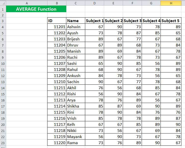
The following image shows the names (column C), IDs (column B), and scores (in five subjects in columns D to H) of 20 students of a class. Given that the maximum marks of each subject are 100, calculate the average score obtained by each student.
Use the AVERAGE function of Excel.
The steps to calculate the average are listed as follows:
Step 1: Enter the following formula in cell I4.
“=AVERAGE(D4:H4)”
So, we have supplied the cell references of row 4 to the AVERAGE function of Excel.

Step 2: Press the “Enter” key. The output in cell I4 is 79.4. Hence, the average score of the student Ashwin is 79.4.

Step 3: Drag the formula of cell I4 till cell I23. For dragging, use the excel fill handleThe fill handle in Excel allows you to avoid copying and pasting each value into cells and instead use patterns to fill out the information. This tiny cross is a versatile tool in the Excel suite that can be used for data entry, data transformation, and many other applications.read more appearing at the bottom-right side of cell I4.
The outputs are shown in the following image. The formula bar shows the formula of the currently selected cell (I23).

Example #3–Average and Maximum Average Revenue by AVERAGE, LOOKUP, and MAX Functions
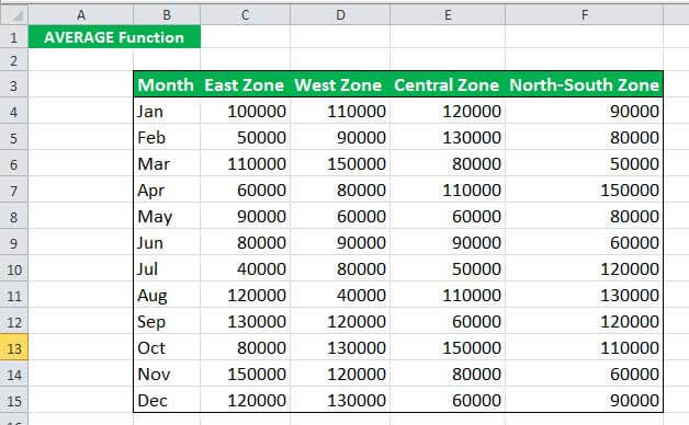
The following image shows the monthly revenuesRevenue is the amount of money that a business can earn in its normal course of business by selling its goods and services. In the case of the federal government, it refers to the total amount of income generated from taxes, which remains unfiltered from any deductions.read more (in $ in columns C to F) generated by an organization from four zones, namely, east, west, central, and north-south. We want to perform the listed tasks:
- Calculate the average revenue for each month.
- Calculate the average revenue for each zone.
- Find the zone with the maximum average revenue.
Use the AVERAGE function of Excel for tasks “a” and “b.” For task “c,” use the LOOKUP and MAX functions. Further, explain the formula used for task “c.”
a. The steps to calculate the average revenue for each month are listed as follows:
Step 1: Enter the following formula in cell C18.
“=AVERAGE(C4:F4)”
Since the average for each row of the dataset needs to be calculated, we have supplied the range reference of row 4.

Step 2: Press the “Enter” key to obtain the output. This is shown in cell C18 of the following image. So, the average revenue for January is $105,000.

Step 3: Drag the formula of cell C18 till cell C29 with the help of the fill handle. The average revenues for all the months are shown in the following image. In this image, the formula bar displays the formula of the currently active cell (C29).

b. The steps to calculate the average revenue for each zone are listed as follows:
Step 1: Enter the following formula in cell G18.
“=AVERAGE(C4:C15)”
This time we supply the cell references of column C in the AVERAGE formula. This is because the average for the entire column needs to be calculated.
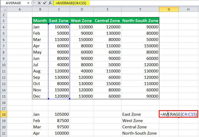
Step 2: Press the “Enter” key. The output of cell G18 is shown in the following image. Likewise, we have entered the following formulas in cells G19, G20, and G21 respectively:
• “=AVERAGE(D4:D15)”
• “=AVERAGE(E4:E15)”
• “=AVERAGE(F4:F15)”
Hence, the averages for each zone have been calculated in the range G18:G21.

c. The steps to find the zone with the maximum average revenue are listed as follows:
Step 1: Enter the following formula in cell H18.
“=LOOKUP(MAX(G18:G21),G18:G21,F18:F21)”
This is shown in the following image.

Step 2: Press the “Enter” key. The output is shown in the following image. Hence, the average revenue of the west zone is maximum.

Explanation of the formula: In the formula of step 1, we have used the vector form of the LOOKUP function. This formula works as follows:
- The MAX functionThe MAX Formula in Excel is used to calculate the maximum value from a set of data/array. It counts numbers but ignores empty cells, text, the logical values TRUE and FALSE, and text values.read more looks for the maximum number of the range G18:G21. The output of the MAX function is 100000. This output becomes the “lookup_value” of the LOOKUP function.
- Next, the LOOKUP functionThe LOOKUP excel function searches a value in a range (single row or single column) and returns a corresponding match from the same position of another range (single row or single column). The corresponding match is a piece of information associated with the value being searched.
read more searches the number 100000 (lookup_value) in the range G18:G21 (lookup_vector). It returns the result from the range F18:F21 (result_vector). So, the given “lookup_value” corresponds with the west zone.
Hence, the output of the formula of step 1 is “west zone.”
Note: The LOOKUP function searches for a value (lookup_value) in a one-row or one-column range (lookup_vector) and returns a corresponding match from the same position of another range (result_vector). The MAX function returns the maximum number from a dataset of numeric values.
For the syntax of the LOOKUP and MAX functions, click the hyperlinks of points “b” and “a” respectively.
Example #4–Average of Top Four Scores by AVERAGE and LARGE Functions
The following image shows the names (column B) and scores (columns C to G) of 16 students in five subjects. We want to perform the listed tasks:
- Calculate the average of five scores of the student Lini (row 4). Use the AVERAGE function of Excel.
- Calculate the average of the top four scores of each student. Use the AVERAGE and LARGE functions of Excel.
Explain the formula used for task “b.”

a. The steps to calculate the average of the five scores of row 4 are listed as follows:
Step 1: Enter the following formula in cell H4.
“=AVERAGE(C4:G4)”

Step 2: Press the “Enter” key. The output is 79.8, as shown in the following image. Hence, Lini’s average of five scores is 79.8.
Note: To find the average (of five scores) for all the students, simply drag the formula of cell H4 till cell H19. For dragging, use the fill handle at the bottom-right corner of cell H4.

b. The steps to calculate the average of the top four scores of each student are listed as follows:
Step 1: Enter the following formula in cell H4.
“=AVERAGE(LARGE(C4:G4,{1,2,3,4}))”
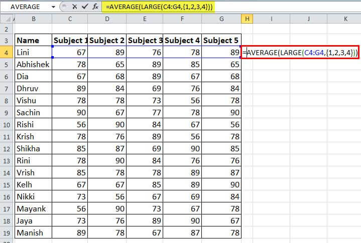
Step 2: Press the “Enter” key. The output is shown in cell H4 of the following image. Hence, Lini’s average of the top four scores is 83.

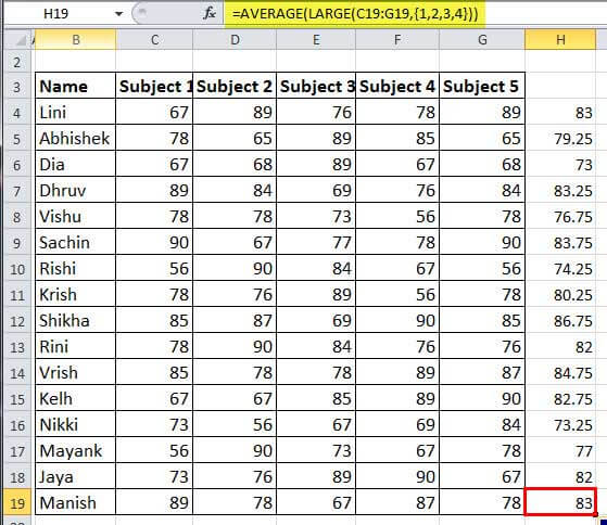
Step 3: Drag the formula of cell H4 till cell H19. The outputs for all rows are shown in the following image. Notice that all these outputs are the averages of the top four scores of each student.
Explanation of the formula: In the formula of step 1, the inner function (LARGE function) is processed first, followed by the outer function (AVERAGE function). This formula works as follows:
- An array of numbers {1,2,3,4} has been supplied to the LARGE functionLARGE Function returns the nth largest value from a given set of values. It is a built-in function of Microsoft Excel and is categorized as a Statistical Excel Function. read more. These numbers represent the position from which values will be returned. So, the LARGE function searches for the first highest, second highest, third highest, and fourth highest values in the range C4:G4. As a result, the LARGE function returns an array of numbers, which is {89,89,78,76}.
- The array of numbers returned by the LARGE function {89,89,78,76} serves as the argument of the AVERAGE function. The AVERAGE function calculates the average of these numbers, which is (89+89+78+76)/4=83.
Likewise, the average of the top four scores has been obtained for all the students of the range B4:B19.
Note: The LARGE function returns a value from the specified position of the supplied range. This position begins from the highest value of the dataset. So, the number 1 corresponds to the maximum value of the dataset, 2 corresponds to the second highest value, 3 corresponds to the third highest value, and so on.
For the syntax of the LARGE function, click the hyperlink given in point “a” of the preceding explanation.
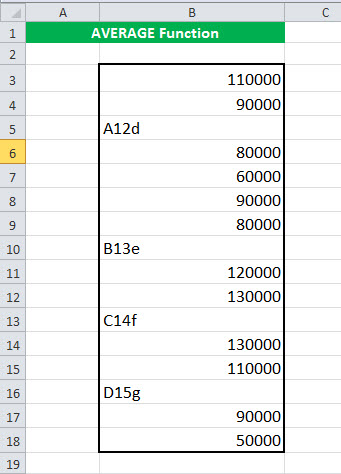
Example #5–Average of Last Three Numbers by AVERAGE, LOOKUP, LARGE, IF, ISNUMBER, and ROW Functions
The following image shows some numeric and textual values in column B. Calculate the average of the last three numeric values, which are in cells B15, B17, and B18.
Use the AVERAGE, LOOKUP, LARGE, IF, ISNUMBER, and ROW functions of Excel. Further, explain the formula used for the given task.
The steps to calculate the average of the last three numeric cells are stated as follows:
Step 1: Enter the following formula in cell C3.
“=AVERAGE(LOOKUP(LARGE(IF(ISNUMBER(B3:B18),ROW(B3:B18)),{1,2,3}),ROW(B3:B18),B3:B18))”

Step 2: Press the keys “Ctrl+Shift+Enter” together. For Excel for Mac, press the keys “Command+Shift+Enter.”
Once the CSE (Ctrl+Shift+Enter) keys are pressed, the formula is enclosed within curly braces. This is shown in the following image. The output is also shown in cell C3.
Hence, the average of the last three numeric values (110000, 90000, and 50000) is 83333.3.

Explanation of the formula: The formula of step 1 works as follows:
a. In the formula “ISNUMBER(B3:B18),ROW(B3:B18),” the ROW functionThe row function in Excel is a worksheet function that displays the current row index number of the selected or target cell. The syntax to use this function is as follows: =ROW( Value ).read more returns the row numbers of the range B3:B18. So, the ROW function returns the following array of values:
{3;4;5;6;7;8;9;10;11;12;13;14;15;16;17;18}.
b. The ISNUMBER functionISNUMBER function in excel is an information function that checks if the referred cell value is numeric or non-numeric.read more processes each value returned by the ROW function. The ISNUMBER function returns “true” if a cell of column B contains a number. It returns “false” if a cell of column B contains a text string. Consequently, the ISNUMBER function returns the following array of logical values:
{TRUE;TRUE;FALSE;TRUE;TRUE;TRUE;TRUE;FALSE;TRUE;TRUE;FALSE;TRUE;TRUE;FALSE;TRUE;TRUE}
c. Next, the IF functionIF function in Excel evaluates whether a given condition is met and returns a value depending on whether the result is “true” or “false”. It is a conditional function of Excel, which returns the result based on the fulfillment or non-fulfillment of the given criteria.
read more operates. The “logical_test” of the IF function is “ISNUMBER(B3:B18)” and the “value_if_true” is “ROW(B3:B18).” The “value_if_false” has been omitted. Therefore, the IF function processes each value of the array returned by the ISNUMBER function. The IF function returns the row number for each “true” value and “false” for each “false” value. So, the IF function returns the following array of values:
{3;4;FALSE;6;7;8;9;FALSE;11;12;FALSE;14;15;FALSE;17;18}
d. The LARGE function has been supplied the array {1,2,3} in the formula “LARGE(IF(ISNUMBER(B3:B18),ROW(B3:B18)),{1,2,3}).” So, the LARGE function searches for the first highest, second highest, and third highest values in the array returned by the IF function. The LARGE function returns the following array of three values:
{18,17,15}
e. Next, the LOOKUP function processes the formula “LOOKUP({18,17,15},ROW(B3:B18),B3:B18).” So, the LOOKUP function searches for the values 18, 17, and 15 in the array returned by the formula “ROW(B3:B18).” The array returned by this ROW formula is the same as that of point “a.” Therefore, the LOOKUP function returns a corresponding match of the values 18, 17, and 15 from the range B3:B18. As a result, the following array is returned by the LOOKUP function:
{50000,90000,110000}
f. Finally, the AVERAGE function calculates the mean of the three values returned by the LOOKUP function. It returns 83333.3 [(50000+90000+110000)/3] as the average.
Notice that the formula of step 1 works as an array formula as it has been completed by pressing the CSE (Ctrl+Shift+Enter) keys. Therefore, the LOOKUP function also returns an array of corresponding matches (50000, 90000, and 110000) for the multiple “lookup_values” (18, 17, and 15) supplied to it.
However, the regular LOOKUP function looks for a single “lookup_value” and returns a single corresponding match. Moreover, it is completed by pressing the “Enter” key.
Note 1: The ROW function returns the row numbers of the supplied cell reference. The ISNUMBER function checks whether the supplied value or cell reference is numeric or not. It returns “true” if the supplied value (or reference) is numeric, otherwise it returns “false.”
The IF function checks whether the supplied condition (logical_test) is true or false. If the condition is true, it returns the “value_if_true.” If the condition is false, it returns the “value_if_false.” If the logical test evaluates to false and the “value_if_false” is omitted, the IF function returns “false.”
For the syntax of the ROW, ISNUMBER, and IF functions, click the hyperlinks given in points “a,” “b,” and “c” of the preceding explanation. The definitions of the LOOKUP and LARGE functions are given in the notes at the end of examples #3 and #4 respectively.
Note 2: To view the array returned by each function, follow the listed steps:
- Select cell C3 that contains the formula.
- Double-click within the selected cell. Alternatively, press the key F2 to enter the Edit mode.
- Select that part of the formula whose array needs to be viewed. For instance, to view the array returned by the ISNUMBER function, select “ISNUMBER(B3:B18).”
- Press the key F9 once a selection has been made in the preceding step.
To stop editing the formula, press the escape (Esc) key.
Frequently Asked Questions
1. Define the AVERAGE function and suggest how to calculate the average in Excel.
The AVERAGE function of Excel calculates the average of the supplied numeric values. The function can be supplied with either direct numbers or references to cells containing numbers. However, the AVERAGE function does not work with text values.
To calculate the average in Excel, follow either of the listed methods:
• Add the numbers of the list manually. Divide the sum obtained by the number of values of the list.
• Open the AVERAGE formula by typing “=AVERAGE” without the beginning and ending double quotation marks. Supply the numbers (enclosed in parentheses) whose average is to be calculated. Press the “Enter” key.
Note: For the syntax of the AVERAGE function, refer to the heading “syntax of the AVERAGE function of Excel,” which is given after the introduction of this article.
2. Define the different varieties of the AVERAGE function of Excel.
In Excel 2007 and the subsequent versions, the following varieties of the AVERAGE function are available:
a. AVERAGEA function–It calculates the average by including the text values (supplied as cell references), Boolean values (true and false), and numeric values. It ignores the empty cells from the count. If the text values are entered directly in the formula, it results in errors. Supplying error values to the formula also causes errors.
b. AVERAGEIF function–It calculates the average of those cells that meet a particular criterion (condition). The criterion, range against which criterion is evaluated, and the actual range to be averaged are supplied to the function as arguments.
c. AVERAGEIFS function–It calculates the average of those cells that meet particular criteria (conditions). This function can be supplied multiple conditions and multiple ranges against which the conditions are to be evaluated. The actual range to be averaged also needs to be supplied as an argument.
Note: The AVERAGEA function of Excel counts the cell references containing text values as zero. It counts “true” and “false” values as 1 and 0 respectively. The AVERAGEA function counts the Boolean values irrespective of whether they are supplied directly or as cell references.
3. Where is the AVERAGE function on the Excel ribbon and how is it used?
The AVERAGE function is within the AutoSum drop-down of the Home tab (“editing” group) and the Formulas tab (“function library” group). To use this function, follow the listed steps:
a. Select the cell immediately below the cells to be averaged.
b. Click the AVERAGE function from the AutoSum drop-down. The AVERAGE formula automatically appears in Excel.
c. Verify the range of the formula and if correct, press the “Enter” key.
The average for the column is returned.
Note 1: Once the AVERAGE formula appears in the selected cell of Excel, its range can be edited manually, if required.
Note 2: To find an average for a row, select the cell to the immediate right of the cells to be averaged. Next, follow the steps “b” and “c” stated above.
AVERAGE Function in Excel Video
Recommended Articles
This has been a guide to the AVERAGE function in Excel. Here we explain how to calculate Average using AVERAGE formula in Excel along with examples and downloadable Excel templates. You may also look at these useful functions of Excel–
- Weighted Average ExcelIn Excel, we calculate Weighted Average by assigning weights to each data set. It is generally used to compute robust observations in statistics or portfolios and is calculated as (w1x1+w2x2+….+wnxn)/(w1+w2+..wn), where w is the weight allocated to the x value and the sumproduct function is used.read more
- LARGE Function in Excel
- Weighted Average Formula
- SUMPRODUCT Function in ExcelThe SUMPRODUCT excel function multiplies the numbers of two or more arrays and sums up the resulting products.read more
Summary – How to use the average function in Excel 2010 Click inside the cell where you want to display the average. Type =AVERAGE(XX:YY) into this cell, but replace XX with the first cell in the range, then replace YY with the last cell in the range. Press Enter on your keyboard to calculate the formula.
Contents
- 1 What is the Excel function for average?
- 2 What is average () function?
- 3 What are the functions of Excel 2010?
- 4 How is average calculated?
- 5 What are the 3 types of averages?
- 6 How do you calculate the average ratio in Excel?
- 7 Is mean same as average in Excel?
- 8 How many functions are there in Excel 2010?
- 9 What are the 5 functions in Excel?
- 10 How many functions in MS Excel?
- 11 What is average computer?
- 12 What is an averaging filter?
- 13 Is there a median IF function in Excel?
- 14 What a function that gets the average of a range of cells?
- 15 What is average of averages called?
- 16 What are the 5 types of averages?
- 17 What are the 4 types of averages?
- 18 What is the percentage formula in Excel?
- 19 What is GCD function in Excel?
- 20 What is ratio formula?
Description. Returns the average (arithmetic mean) of the arguments. For example, if the range A1:A20 contains numbers, the formula =AVERAGE(A1:A20) returns the average of those numbers.
What is average () function?
The AVERAGE function in Excel calculates the average (arithmetic mean) of a group of numbers. The AVERAGE function ignores logical values, empty cells and cells that contain text.
What are the functions of Excel 2010?
Excel functions (alphabetical)
| Function name | Type and description |
|---|---|
| FORECAST.LINEAR function | Statistical: Returns a future value based on existing values |
| FORMULATEXT function | Lookup and reference: Returns the formula at the given reference as text |
How is average calculated?
The average of a set of numbers is simply the sum of the numbers divided by the total number of values in the set. For example, suppose we want the average of 24 , 55 , 17 , 87 and 100 . Simply find the sum of the numbers: 24 + 55 + 17 + 87 + 100 = 283 and divide by 5 to get 56.6 .
What are the 3 types of averages?
There are three main types of average: mean, median and mode.
How do you calculate the average ratio in Excel?
How to Calculate the Ratio in Excel. Calculate Ratio Formula: To calculate the Ratio in excel, the Shop 1 will be divided by GCD and the Shop 2 will be divided by GCD. You can place a colon between those two numbers. Example: To see the ratio, enter this formula in cell E2 = B2/GCD(B2,C2)&”:”&C2/GCD(B2,C2).
Is mean same as average in Excel?
The mean or the statistical mean is essentially means average value and can be calculated by adding data points in a setand then dividing the total, by the number of points. Excel’s AVERAGE function does exactly this: sum all the values and divides the total by the count of numbers.
How many functions are there in Excel 2010?
In Excel 2010: Advanced Formulas and Functions, author Dennis Taylor demystifies formulas and some of the most challenging of the nearly 400 functions in Excel and shows how to put them to their best use.
What are the 5 functions in Excel?
5 Functions of Excel/Sheets That Every Professional Should Know
- VLookup Formula.
- Concatenate Formula.
- Text to Columns.
- Remove Duplicates.
- Pivot Tables.
How many functions in MS Excel?
Though every Excel feature has a use case, no single person uses every Excel feature themselves. Cut through the 500+ functions, and you’re left with 100 or so truly useful functions and features for the majority of modern knowledge workers.
What is average computer?
Updated: 08/02/2020 by Computer Hope. Alternatively referred to as the arithmetic mean, an average is the sum of a series of numbers, divided by the total amount of numbers.
What is an averaging filter?
Average Filtering. Average (or mean) filtering is a method of ‘smoothing’ images by reducing the amount of intensity variation between neighbouring pixels. The average filter works by moving through the image pixel by pixel, replacing each value with the average value of neighbouring pixels, including itself.
Is there a median IF function in Excel?
The MEDIAN function finds the middle value out of a set of numbers.The array formula lets the IF function test for multiple conditions in a single cell. When the condition is met, the array formula determines what data the MEDIAN function will examine to find the middle award amount.
What a function that gets the average of a range of cells?
The Microsoft Excel AVERAGEIF function returns the average (arithmetic mean) of all numbers in a range of cells, based on a given criteria. The AVERAGEIF function is a built-in function in Excel that is categorized as a Statistical Function.
What is average of averages called?
Calculating a Weighted Average (Average of Averages)
What are the 5 types of averages?
Averages
- Mean. Mean. This is the sum (total) of all the numbers, divided by how many numbers there are in the list. Mean ›
- Median. Median. This is the middle number in the list. Median ›
- Mode. Mode. This is the number that appears most often in the list.
- Range. The range shows the spread of numbers in a list or set. Range ›
What are the 4 types of averages?
We consider there to be four types of average: mean, mode, median and range. Actually, range is a measure of spread or distribution but the others are our most common “measures of central tendency”.
What is the percentage formula in Excel?
The percentage formula in Excel is = Numerator/Denominator (used without multiplication by 100). To convert the output to a percentage, either press “Ctrl+Shift+%” or click “%” on the Home tab’s “number” group. Let us consider a simple example.
What is GCD function in Excel?
The Excel GCD function returns the greatest common divisor of two or more integers. The greatest common divisor is the largest integer that goes into all supplied numbers without a remainder. For example, =GCD(60,36) returns 12.
What is ratio formula?
The ratio formula for any two quantities say a and b is given as, a:b = a/b. Since a and b are individual amounts for two quantities, the total quantity combined is given as (a + b). Let us understand the ratio formula better using a few solved examples.
AVERAGE and AVERAGEA functions are used to calculate the arithmetic average of the arguments of interest in Excel. The average is calculated in the classical way — summing all the numbers and dividing the sum by the number of these numbers. The main difference between these functions is that they process differently non-numeric types of values that are in Excel cells. More about everything in more detail.
Examples of using the AVERAGE function in Excel
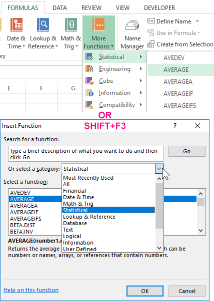
AVERAGE function refers to the Statistical group. Therefore, to call this function in Excel, you must select the tool: “FORMULAS” — “Functions Library” — “More functions” — “Statistical” — “AVERAGE”. Or call the «Insert Function» dialog box (SHIFT + F3) and select the «Statistical» option from the «Category:» drop-down list. After that, in the “Select function:” field there will be a list of categories with statistical functions where the AVERAGE is located, as well as AVERAGEA.
If there is a range of B2:B8 cells with numbers, then the formula =AVERAGE(B2:B8) will return the average value of the given numbers in this range:
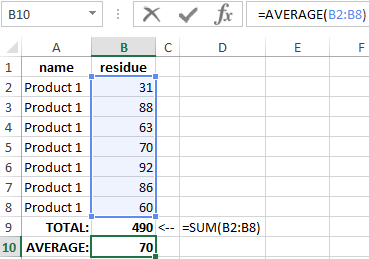
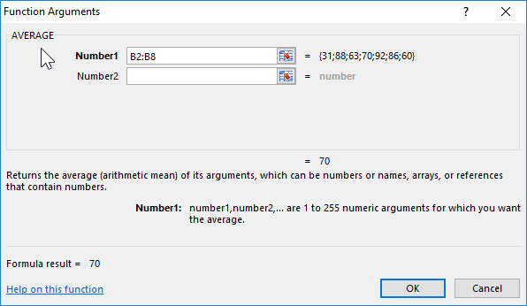
The syntax is the following: =AVERAGE(number1,[number2],…), where the first number is a required argument, and all subsequent arguments (up to the number 255) are optional for filled. That is, the number of selected source ranges cannot exceed more than 255:
The argument can have a numeric value, be a reference to a range or array. Text and logical values in the range are completely ignored.
The arguments of the AVERAGE function can be represented not only by numbers, but also by names or references to a specific range (cell) containing a number. The logical value and textual representation of the number, which is directly entered into the argument list, is taken into account.
If the argument is represented by a reference to a range (cell), then its text or logical value (reference to an empty cell) is ignored. In this case, cells that contain zero are counted. If the argument contains errors or text that cannot be converted to a number, then this results in a common error. To take into account logical values and the textual representation of numbers, it is necessary to use in the calculations the AVERAGEA function, which will be discussed further.
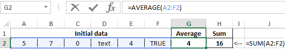
The result of the function in the example in the picture below is the number 4, since logical and text objects are ignored. Therefore:
(5 + 7 + 0 + 4) / 4 = 4
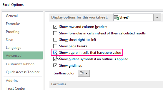
When calculating averages, you need to take into account the difference between a blank cell and a cell containing a zero value, especially if the «Show a zero in cells that have zero values» option is cleared in the Excel dialog box. When checked, empty cells are ignored, but zero values are not. To remove or set this flag, open the “FILE” tab, then click on “Options” and select in the category “Advanced” group “Display options for this worksheet:”, where it is possible to check the box:
The results of another 4 tasks are summarized in the table below:
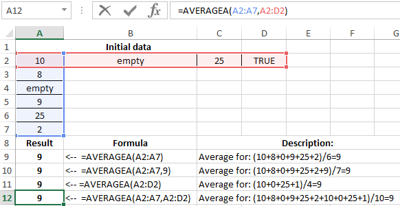
As you can see in the example, in cell A9, the AVERAGE function has 2 arguments: 1 — a range of cells, 2 — an additional number 5. The same can be specified in the arguments and additional ranges of cells with numbers. For example, as in cell A11.
Formulas with examples of using the AVERAGEA function
AVERAGEA function differs from AVERAGE in that the true logical value of “TRUE” in the range is equal to 1, and the false logical value of “FALSE” or the text value in the cells is equal to zero. Therefore, the result of calculating the AVERAGEA function is different:
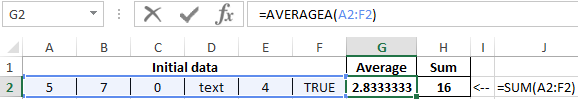
The result of the function returns the number in the example 2,833333, since the text and logical values are taken as zero, and the logical TRUE is equal to one. Consequently:
(5 + 7 + 0 + 0 + 4 + 1) / 6 = 2.83
Syntax:
=AVERAGEA(value1,[value2],…)
The arguments of the AVERAGEA function are subject to the following properties:
- «Value1» is mandatory, and «value2» and all values that follow it are optional. The total number of cell ranges or their values can be from 1 to 255 cells.
- The argument can be a number, a name, an array, or a reference containing a number, as well as a textual representation of the number or a logical value, for example, “true” or “false”.
- The logical value and textual representation of the number entered in the argument list is taken into account.
- An argument containing the value “true” is interpreted as 1. An argument containing the value “false” is interpreted as 0 (zero).
- Text contained in arrays and references is interpreted as 0 (zero). An empty text («») is also interpreted as 0 (zero).
- If the argument is an array or reference, then only the values included in this array or reference are used. Empty cells and text in the array and reference are ignored.
- Arguments that are error values or text that cannot be converted to numbers cause errors.
The results of the feature of AVERAGEA are summarized in the table below:
Download examples with functions AVERAGE for Excel
Attention! When calculating the mean values in Excel, you need to take into account the differences between a blank cell and a cell containing a zero value (especially if the “Show a zero in cells that have zero values” in “Option” is unchecked in the options dialog box). When checked, empty cells are not counted, and zero values are counted. To check the box on the “FILE” tab, select the “Option” command, go to the “Advanced” category, where find the section “Show options for the next sheet” and set the flag there.
На чтение 1 мин
Функция СРЗНАЧ в Excel используется для вычисления среднего арифметического из заданного диапазона данных.
Содержание
- Что возвращает функция
- Синтаксис
- Аргументы функции
- Дополнительная информация
- Примеры использования функции СРЗНАЧ в Excel
Что возвращает функция
Возвращает число, соответствующее среднему арифметическому от заданного диапазона данных.
 Больше лайфхаков в нашем Telegram Подписаться
Синтаксис
=AVERAGE(number1, [number2], …) — английская версия
=СРЗНАЧ(число1;[число2];…) — русская версия
Аргументы функции
- number1 (число1) — первое число, диапазон чисел, из которого необходимо вычислить среднее арифметическое;
- [number2] ([число2]) (Опционально) — второе число, диапазон чисел, из которого необходимо вычислить среднее арифметическое. Максимальное количество аргументов функции — 255.
Дополнительная информация
- Аргументами функции СРЗНАЧ (AVERAGE) в Excel могут быть числа, именованные диапазоны, ссылки на ячейки, содержащие числовые значения;
- Ссылки на ячейки содержащими текст, логические значения или пустые ячейки игнорируются функцией. Вместе с тем, ячейки со значением «0» учитываются при вычислении среднего арифметического;
- Учитываются логические значения и текстовые представления чисел, которые вы вводите непосредственно в список аргументов;
- Аргументы с ошибками не могут быть учтены и использованы при работе функции.
Примеры использования функции СРЗНАЧ в Excel
How to Calculate Average in Excel (With Formula Examples)
What is average? It is simply the arithmetic mean of a given set of numbers.
Averages are super easy to calculate – no doubt about that 🎉
But if your dataset gets long, it might be that easy to calculate averages manually. And who would want to spend hours on something worth a few clicks only?
Excel offers a multitude of ways to calculate averages in Excel. And we will look into them all.
So what are we waiting for? Let’s jump right into the guide below.
Also, download our free sample workbook here to tag along with the guide as you continue reading 📩
First of all other methods, Excel offers an in-built AVERAGE function to calculate averages.
Want to see how the AVERAGE function works in Excel? Let’s go 🚗
The image below shows the marks of a student in different subjects.

The total marks for all the subjects are 100. So how much did Nica score overall (on average)? To calculate that.
- Activate a cell and start writing the AVERAGE function as follows:
= AVERAGE (

When you average cells in Excel, know that the AVERAGE function will ignore logical values and empty cells but include any cells containing zero values 0️⃣
- Specify the data range that is to be averaged.
= AVERAGE (B2:B7)

Pro Tip!
You can specify the data range as cell references like = AVERAGE (B2, B3, B4, B5, B6, B7).
Or you can write this argument as a reference to a whole cell range like = AVERAGE (B2:B7).
And if you don’t have the figures populated in cells, you can write the values inside the function yourself as = AVERAGE (10, 12).
- Press Enter, and you’re good to go.

Nica scored 82 marks on average. That’s a good score by the way 🥇
Calculate the average with a formula
We’ve tried using the AVERAGE function of Excel to calculate averages. It’s now time for something more interesting.
Pro Tip!
Do you know what is meant by average? Average is the sum of a given set of numbers divided by the count of those numbers 👩🏫
For example, what is the average of 2,4, and 6?
Count the numbers. There are 3 of them.
Divide the sum by the count (12/3 = 4).
Can we write our formula to calculate the average in Excel? Certainly yes. Let’s again calculate the average marks for Nica with a formula.
- Add up all the marks by writing the following formula.
= (B2 + B3 + B4 + B5 + B6 + B7)

- Divide the formula above by the number of values.
We have 6 subject marks here, so we will divide the formula above by 6 6️⃣
= (B2 + B3 + B4 + B5 + B6 + B7) / 6

- Press Enter to get the average marks as below.

82 – same as above! This tells that the AVERAGE function does nothing different than what we did above 👆
Calculate the average with the SUM and COUNT formula
The ways for calculating averages in Excel have yet not ended. You can calculate averages by combining other functions of Excel.
For example, the functions SUM and COUNT. How? Let’s see here 👀
We are again calculating the average marks for Nica (yes, once again), but this time with a different method. So let’s begin.
- Write the SUM function as follows:
= SUM (B2:B7)

The SUM function will sum up all the marks ➕
- Divide the above formula by the COUNT function as follows:
= SUM (B2:B7) / COUNT (B2:B7)

The COUNT function counts the number of values in the referred cell range.
The COUNT function counts all the cells in the defined cell range. As we have defined the cell range B2:B7, it will count the cells between B2 to B7.
- Press Enter to get the following results.

And there it is! Excel computes the AVERAGE of the given numbers.
Easy, no 😍
That’s it – Now what?
And that’s how you can calculate averages in Excel. It is super simple – and now you know that too. There are multiple ways how you can calculate averages in Excel.
Using a formula, the SUM and COUNT formula, and obviously, through the AVERAGE function in Excel.
However, just like calculating averages, there’s so much more that you can do in Excel using other functions. Some of my go-to Excel functions include the VLOOKUP, SUMIF, and IF functions of Excel.
These functions would make your life a lot easier. I suggest you learn them right away ✈
But How? My 30-minute free email course will help you learn them (and many more) Excel functions in no time.
Other resources
There’s not only one function dedicated to calculating averages in Excel – but much more. Like the AVERAGEA function, AVERAGEIF function, and AVERAGEIFS function. Learn them here.
You’d also be surprised to know that Excel doesn’t offer an in-built function to calculate weighted average. But you can still calculate it in Excel using other functions. How? Learn here.
Frequently asked questions
To calculate the average percentage in Excel:
- The source data must be in percentages.
- Use the AVERAGE function to calculate the average of the given percentages.
Apply the “Percentage” format to the cell containing the Average from the Home Tab > Number > Percentage.
Kasper Langmann2023-02-23T11:10:47+00:00
Page load link
In this article, we will learn How to use the AVERAGE function in Excel.
What is AVERAGE or MEAN? And What type of Excel functions use it?
AVERAGEA function is a built-in function to calculate the average or mean of the range of data values provided. The average or mean for the set of values is calculated using the formula shown below.
Here
- Sum of numbers is the mathematical addition of values.
- Count of numbers (n) is the total count of values considered.
There are newer and updated versions of AVERAGE function used for a different set of dataset values.
- AVERAGEA function : This function is used for values considering text as 0, TRUE as 1 and FALSE as 0 and numbers in text format.
- AVERAGE function : This function is used for values considering only numbers which are in number format.
- AVERAGEIF function : This function takes the average of values in range applying any one condition over the corresponding or the same range.
- AVERAGEIFS function : This function takes the average of values in range applying any multiple condition over the corresponding or the same range.
AVERAGE Function in Excel
AVERAGE function calculates the average of the input array numbers ignoring text and logic values.
AVERAGE function Syntax:
array : input multiple number as array reference with the function. Like values at array A5:A500.
Example :
All of these might be confusing to understand. Let’s understand how to use the function using an example.
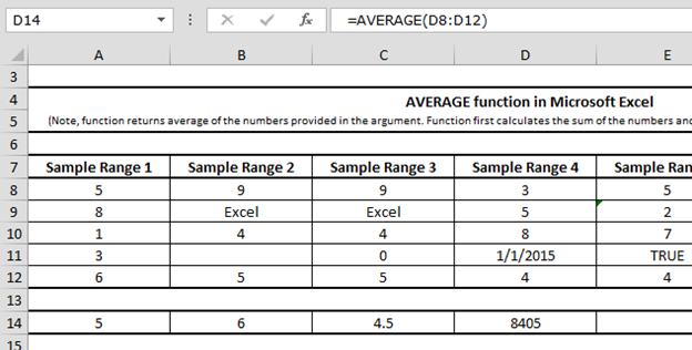
Refer to these 7 different examples for the usage of Average function in Microsoft Excel on the basis of following sample data:
1st Example:
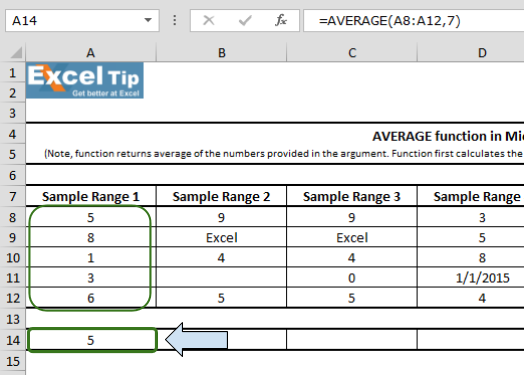
In the sample 1 we have few numbers for which we want to calculate average. Follow the steps given below:
- Enter AVERAGE function in cell A14
- =AVERAGE(A8:A12,7)
- Press Enter
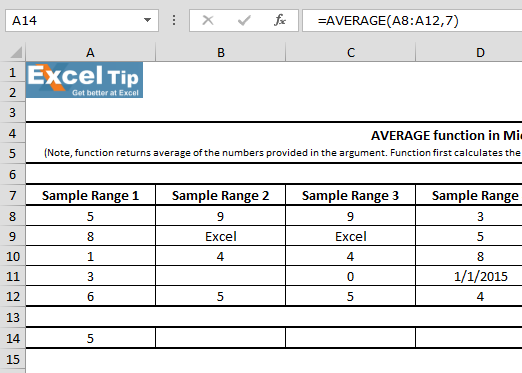
Note: It can take up to 255 number of arguments in Excel 2007 or later versions.
Formula Explanation: A8 to A12 as range in the first argument, then we close the parentheses and hit enter. The function returns 4.6 as the average of these 5 numbers. Also, if you sum up these numbers 5 + 8 + 1 + 3 + 6 it will be equal to 23. And, as we have 5 numbers of cells in the argument, and when we divide 23 by 5, it returns 4.6 which is an average.
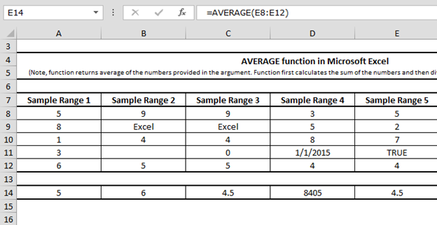
2nd Example:
In this example, we’ll see how AVERAGE function handles any empty cell or cells that contain text in the range, follow the steps given below:
- Enter AVERAGE function in cell B14
- Then, select B8:B12 as range
- =AVERAGE(B8:B12)
- Press Enter
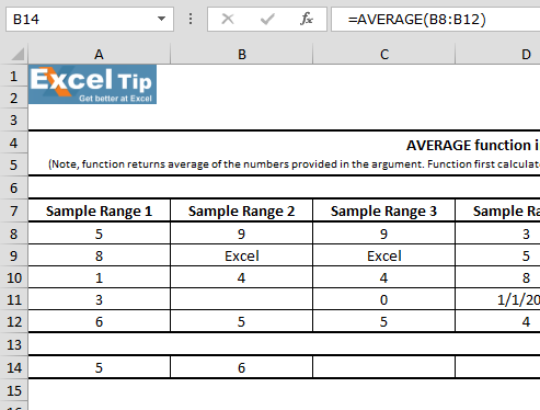
Formula Explanation: In this case function returns 6 as average. Because cell B9 is ignored by AVERAGE function, since it contains text instead of a number and function found no value in B11.
3rd Example:
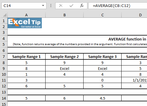
In this example, we’ll learn if there is a cell that contains zero in the range. Follow the steps given below:
- Enter function in cell C14
- Select C8 to C12 range
- =AVERAGE(C8:C12)
- Press Enter
4th Example:
In this example, we can see that one of the cell contains date within a range. So, we’ll learn that how Average function will work in case of any cell that contains date.
Follow given below steps:
- Enter the function in cell D14
- =AVERAGE(D8:D12)
- Press Enter
Function returns 8405. It is because in Excel, dates are saved as numbers. In this example, we have taken 1st Jan,2015 which is equivalent to 42005
5th Example:
In this example, we have taken text in the range for which we want to calculate average.
Follow the steps given below:
- Enter the function in cell E14
- =AVERAGE(E8:E12)
- Press Enter
- Function returns 4.5 as result
It means Average function does not consider text value while performing the calculation. And by doing so it provides accurate results.
6th Example:
In this example, we’ll learn if a cell is having #N/A error within a range for which we want to calculate average, then how Average function will perform.
Follow the steps given below:
- Enter the function in cell F14
- =AVERAGE(F8:F12)
- Press Enter
- Function will return #N/A as result
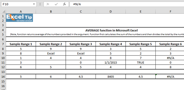
If any cell contains an error, the formula would also return error.
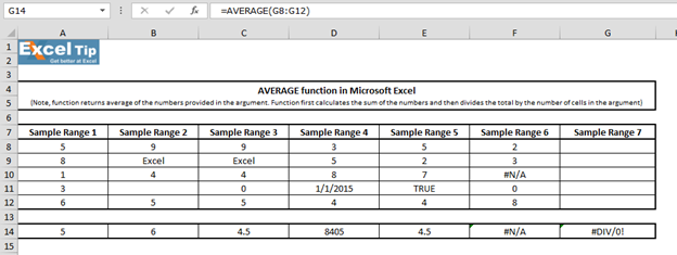
7th Example:
In this example, we’ll check if the selected range for average function is blank and how Average function will work.
Follow the steps given below:
- Enter the function in cell G14
- =AVERAGE(G8:G12)
- Press Enter
The function will return #DIV/0! Error because function did not find any value to be averaged in the argument.
In this way we can make use of the average function in MS-Excel.
Here are all the observational notes using the AVERAGE function in Excel
Notes :
- The function returns #VALUE! criteria if no value matches the given criteria.
Video: How to use AVERAGE function in Excel
Watch the steps in this short video, and the written instructions are above the video
Hope this article about How to use the AVERAGE function in Excel is explanatory. You can use these functions in Excel 2016, 2013 and 2010. Find more articles on Mathematical operation and formulation with different criteria.
If you liked our blogs, share it with your friends on Facebook. And also you can follow us on Twitter and Facebook. We would love to hear from you, do let us know how we can improve, complement or innovate our work and make it better for you. Write us at info@exceltip.com
Related Articles :
How to use the AVERAGEIF function in Excel : This function takes the average of values in range applying any one condition over the corresponding or the same range.
How to use the AVERAGEIFS function in Excel : This function takes the average of values in range applying any multiple conditions over the corresponding or the same range.
How To Highlight Cells Above and Below Average Value : highlight values which are above or below the average value using the conditional formatting in Excel.
Ignore zero in the Average of numbers : calculate the average of numbers in the array ignoring zeros using AVERAGEIF function in Excel.
Calculate Weighted Average : find the average of values having different weight using SUMPRODUCT function in Excel.
Average Difference between lists : calculate the difference in average of two different lists. Learn more about how to calculate average using basic mathematical average formula.
Average numbers if not blank in Excel : extract average of values if cell is not blank in excel.
AVERAGE of top 3 scores in a list in excel : Find the average of numbers with criteria as highest 3 numbers from the list in Excel
Popular Articles :
How to use the IF Function in Excel : The IF statement in Excel checks the condition and returns a specific value if the condition is TRUE or returns another specific value if FALSE.
How to use the VLOOKUP Function in Excel : This is one of the most used and popular functions of excel that is used to lookup value from different ranges and sheets.
How to use the SUMIF Function in Excel : This is another dashboard essential function. This helps you sum up values on specific conditions.
How to use the COUNTIF Function in Excel : Count values with conditions using this amazing function. You don’t need to filter your data to count specific values. Countif function is essential to prepare your dashboard.