What is text functions in excel

The TEXT function lets you change the way a number appears by applying formatting to it with format codes. It’s useful in situations where you want to display numbers in a more readable format, or you want to combine numbers with text or symbols.

Note: The TEXT function will convert numbers to text, which may make it difficult to reference in later calculations. It’s best to keep your original value in one cell, then use the TEXT function in another cell. Then, if you need to build other formulas, always reference the original value and not the TEXT function result.

Syntax

TEXT(value, format_text)

The TEXT function syntax has the following arguments:

Argument Name	Description
value	A numeric value that you want to be converted into text.
format_text	A text string that defines the formatting that you want to be applied to the supplied value.

Overview

In its simplest form, the TEXT function says:

=TEXT(Value you want to format, «Format code you want to apply»)

Here are some popular examples, which you can copy directly into Excel to experiment with on your own. Notice the format codes within quotation marks.

Formula	Description
=TEXT(1234.567,«$#,##0.00»)	Currency with a thousands separator and 2 decimals, like $1,234.57. Note that Excel rounds the value to 2 decimal places.
=TEXT(TODAY(),«MM/DD/YY»)	Today’s date in MM/DD/YY format, like 03/14/12
=TEXT(TODAY(),«DDDD»)	Today’s day of the week, like Monday
=TEXT(NOW(),«H:MM AM/PM»)	Current time, like 1:29 PM
=TEXT(0.285,«0.0%»)	Percentage, like 28.5%
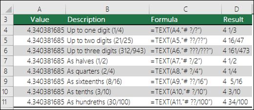
=TEXT(4.34 ,«# ?/?»)	Fraction, like 4 1/3
=TRIM(TEXT(0.34,«# ?/?»))	Fraction, like 1/3. Note this uses the TRIM function to remove the leading space with a decimal value.
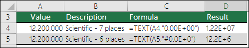
=TEXT(12200000,«0.00E+00»)	Scientific notation, like 1.22E+07
=TEXT(1234567898,«[<=9999999]###-####;(###) ###-####»)	Special (Phone number), like (123) 456-7898
=TEXT(1234,«0000000»)	Add leading zeros (0), like 0001234
=TEXT(123456,«##0° 00′ 00»»)	Custom — Latitude/Longitude

Note: Although you can use the TEXT function to change formatting, it’s not the only way. You can change the format without a formula by pressing CTRL+1 (or +1 on the Mac), then pick the format you want from the Format Cells > Number dialog.

Download our examples

You can download an example workbook with all of the TEXT function examples you’ll find in this article, plus some extras. You can follow along, or create your own TEXT function format codes.

Download Excel TEXT function examples

Other format codes that are available

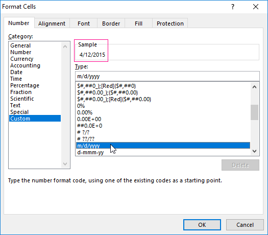
You can use the Format Cells dialog to find the other available format codes:

Press Ctrl+1 (+1 on the Mac) to bring up the Format Cells dialog.
Select the format you want from the Number tab.
Select the Custom option,
The format code you want is now shown in the Type box. In this case, select everything from the Type box except the semicolon (;) and @ symbol. In the example below, we selected and copied just mm/dd/yy.
Press Ctrl+C to copy the format code, then press Cancel to dismiss the Format Cells dialog.
Now, all you need to do is press Ctrl+V to paste the format code into your TEXT formula, like: =TEXT(B2,»mm/dd/yy«). Make sure that you paste the format code within quotes («format code»), otherwise Excel will throw an error message.

Format codes by category

Following are some examples of how you can apply different number formats to your values by using the Format Cells dialog, then use the Custom option to copy those format codes to your TEXT function.

Why does Excel delete my leading 0’s?

Excel is trained to look for numbers being entered in cells, not numbers that look like text, like part numbers or SKU’s. To retain leading zeros, format the input range as Text before you paste or enter values. Select the column, or range where you’ll be putting the values, then use CTRL+1 to bring up the Format > Cells dialog and on the Number tab select Text. Now Excel will keep your leading 0’s.

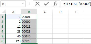
If you’ve already entered data and Excel has removed your leading 0’s, you can use the TEXT function to add them back. You can reference the top cell with the values and use =TEXT(value,»00000″), where the number of 0’s in the formula represents the total number of characters you want, then copy and paste to the rest of your range.

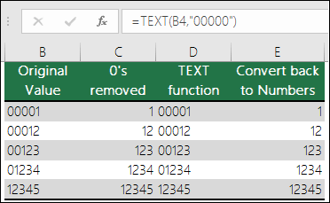
If for some reason you need to convert text values back to numbers you can multiply by 1, like =D4*1, or use the double-unary operator (—), like =—D4.

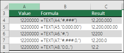
Excel separates thousands by commas if the format contains a comma (,) that is enclosed by number signs (#) or by zeros. For example, if the format string is «#,###», Excel displays the number 12200000 as 12,200,000.

A comma that follows a digit placeholder scales the number by 1,000. For example, if the format string is «#,###.0,», Excel displays the number 12200000 as 12,200.0.

Notes:

The thousands separator is dependent on your regional settings. In the US it’s a comma, but in other locales it might be a period (.).
The thousands separator is available for the number, currency and accounting formats.

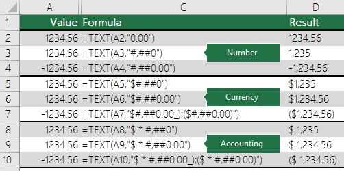
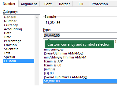
Following are examples of standard number (thousands separator and decimals only), currency and accounting formats. Currency format allows you to insert the currency symbol of your choice and aligns it next to your value, while accounting format will align the currency symbol to the left of the cell and the value to the right. Note the difference between the currency and accounting format codes below, where accounting uses an asterisk (*) to create separation between the symbol and the value.

To find the format code for a currency symbol, first press Ctrl+1 (or +1 on the Mac), select the format you want, then choose a symbol from the Symbol drop-down:

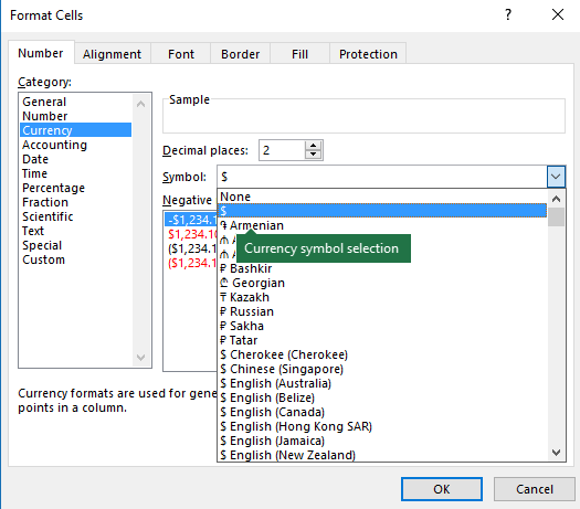
Then click Custom on the left from the Category section, and copy the format code, including the currency symbol.

Note: The TEXT function does not support color formatting, so if you copy a number format code from the Format Cells dialog that includes a color, like this: $#,##0.00_);[Red]($#,##0.00), the TEXT function will accept the format code, but it won’t display the color.

You can alter the way a date displays by using a mix of «M» for month, «D» for days, and «Y» for years.

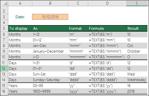
Format codes in the TEXT function aren’t case sensitive, so you can use either «M» or «m», «D» or «d», «Y» or «y».

You can alter the way time displays by using a mix of «H» for hours, «M» for minutes, or «S» for seconds, and «AM/PM» for a 12-hour clock.

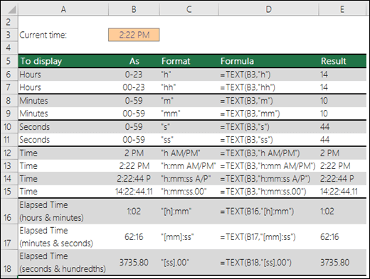
If you leave out the «AM/PM» or «A/P», then time will display based on a 24-hour clock.

Format codes in the TEXT function aren’t case sensitive, so you can use either «H» or «h», «M» or «m», «S» or «s», «AM/PM» or «am/pm».

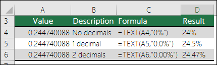
You can alter the way decimal values display with percentage (%) formats.

You can alter the way decimal values display with fraction (?/?) formats.

Scientific notation is a way of displaying numbers in terms of a decimal between 1 and 10, multiplied by a power of 10. It is often used to shorten the way that large numbers display.

Excel provides 4 special formats:

Zip Code — «00000»
Zip Code + 4 — «00000-0000»
Phone Number — «[<=9999999]###-####;(###) ###-####»
Social Security Number — «000-00-0000»

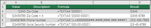
Special formats will be different depending on locale, but if there aren’t any special formats for your locale, or if these don’t meet your needs then you can create your own through the Format Cells > Custom dialog.

Common scenario

The TEXT function is rarely used by itself, and is most often used in conjunction with something else. Let’s say you want to combine text and a number value, like “Report Printed on: 03/14/12”, or “Weekly Revenue: $66,348.72”. You could type that into Excel manually, but that defeats the purpose of having Excel do it for you. Unfortunately, when you combine text and formatted numbers, like dates, times, currency, etc., Excel doesn’t know how you want to display them, so it drops the number formatting. This is where the TEXT function is invaluable, because it allows you to force Excel to format the values the way you want by using a format code, like «MM/DD/YY» for date format.

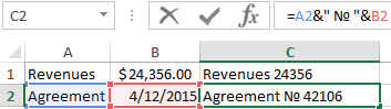
In the following example, you’ll see what happens if you try to join text and a number without using the TEXT function. In this case, we’re using the ampersand (&) to concatenate a text string, a space (» «), and a value with =A2&» «&B2.

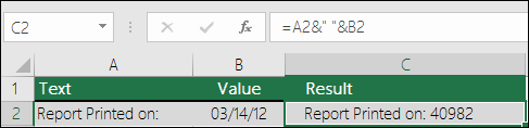
As you can see, Excel removed the formatting from the date in cell B2. In the next example, you’ll see how the TEXT function lets you apply the format you want.

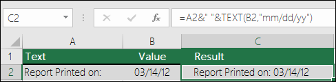
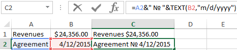
Our updated formula is:

Cell C2:=A2&» «&TEXT(B2,»mm/dd/yy») — Date format

Frequently Asked Questions

Yes, you can use the UPPER, LOWER and PROPER functions. For example, =UPPER(«hello») would return «HELLO».

Yes, but it takes a few steps. First, select the cell or cells where you want this to happen and use Ctrl+1 to bring up the Format > Cells dialog, then Alignment > Text control > check the Wrap Text option. Next, adjust your completed TEXT function to include the ASCII function CHAR(10) where you want the line break. You might need to adjust your column width depending on how the final result aligns.

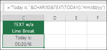
In this case, we used: =»Today is: «&CHAR(10)&TEXT(TODAY(),»mm/dd/yy»)

This is called Scientific Notation, and Excel will automatically convert numbers longer than 12 digits if a cell(s) is formatted as General, and 15 digits if a cell(s) is formatted as a Number. If you need to enter long numeric strings, but don’t want them converted, then format the cells in question as Text before you input or paste your values into Excel.

Function	Description
ARRAYTOTEXT function	Returns an array of text values from any specified range
ASC function	Changes full-width (double-byte) English letters or katakana within a character string to half-width (single-byte) characters
BAHTTEXT function	Converts a number to text, using the ß (baht) currency format
CHAR function	Returns the character specified by the code number
CLEAN function	Removes all nonprintable characters from text
CODE function	Returns a numeric code for the first character in a text string
CONCAT function	Combines the text from multiple ranges and/or strings, but it doesn’t provide the delimiter or IgnoreEmpty arguments.
CONCATENATE function	Joins several text items into one text item
DBCS function	Changes half-width (single-byte) English letters or katakana within a character string to full-width (double-byte) characters
DOLLAR function	Converts a number to text, using the $ (dollar) currency format
EXACT function	Checks to see if two text values are identical
FIND, FINDB functions	Finds one text value within another (case-sensitive)
FIXED function	Formats a number as text with a fixed number of decimals
LEFT, LEFTB functions	Returns the leftmost characters from a text value
LEN, LENB functions	Returns the number of characters in a text string
LOWER function	Converts text to lowercase
MID, MIDB functions	Returns a specific number of characters from a text string starting at the position you specify
NUMBERVALUE function	Converts text to number in a locale-independent manner
PHONETIC function	Extracts the phonetic (furigana) characters from a text string
PROPER function	Capitalizes the first letter in each word of a text value
REPLACE, REPLACEB functions	Replaces characters within text
REPT function	Repeats text a given number of times
RIGHT, RIGHTB functions	Returns the rightmost characters from a text value
SEARCH, SEARCHB functions	Finds one text value within another (not case-sensitive)
SUBSTITUTE function	Substitutes new text for old text in a text string
T function	Converts its arguments to text
TEXT function	Formats a number and converts it to text
TEXTAFTER function	Returns text that occurs after given character or string
TEXTBEFORE function	Returns text that occurs before a given character or string
TEXTJOIN function	Combines the text from multiple ranges and/or strings
TEXTSPLIT function	Splits text strings by using column and row delimiters
TRIM function	Removes spaces from text
UNICHAR function	Returns the Unicode character that is references by the given numeric value
UNICODE function	Returns the number (code point) that corresponds to the first character of the text
UPPER function	Converts text to uppercase
VALUE function	Converts a text argument to a number
VALUETOTEXT function	Returns text from any specified value

What is the Excel TEXT Function?

The Excel TEXT Function[1] is used to convert numbers to text within a spreadsheet. Essentially, the function will convert a numeric value into a text string. TEXT is available in all versions of Excel.

Formula

=Text(Value, format_text)

Where:

Value is the numerical value that we need to convert to text

Format_text is the format we want to apply

When is the Excel TEXT Function required?

We use the TEXT function in the following circumstances:

When we want to display dates in a specified format
When we wish to display numbers in a specified format or in a more legible way
When we wish to combine numbers with text or characters

Examples

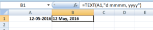
1. Basic example – Excel Text Function

With the following data, I need to convert the data to “d mmmm, yyyy” format. When we insert the text function, the result would look as follows:

2. Using Excel TEXT with other functions

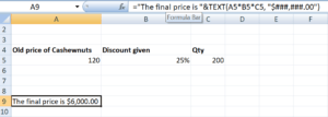
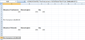
We use the old price and the discount given in cells A5 and B5. The quantity is given in C5. We wish to show some text along with the calculations. We wish to display the information as follows:

The final price is $xxx

Where xxx would be the price in $ terms.

For this, we can use the formula:

=”The final price is “&TEXT(A5*B5*C5, “$###,###.00”)

The other way to do it by using the CONCATENATE function as shown below:

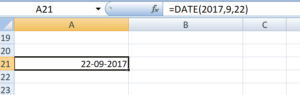
3. Combining the text given with data using TEXT function

When I use the date formula, I would get the result below:

Now, if we try to combine today’s date using CONCATENATE, Excel would give a weird result as shown below:

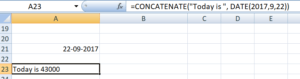
What happened here was that dates that are stored as numbers by Excel were returned as numbers when the CONCATENATE function is used.

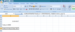
How to fix it?

To fix it, we need to use the Excel TEXT function. The formula to be used would be:

4. Adding zeros before numbers with variable lengths

We all know any zero’s added before numbers are automatically removed by Excel. However, if we need to keep those zeros then the TEXT function comes handy. Let’s see an example to understand how to use this function.

We are given a 9-digit product code, but Excel removed the zeros before it. We can use TEXT as shown below and convert the product code into a 9-digit number:

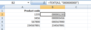
In the above formula, we are given the format code containing 9-digit zeros, where the number of zeros is equal to the number of digits we wish to display.

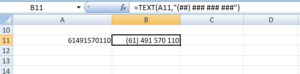
5. Converting telephone numbers to a specific format

If we wish to do the same for telephone numbers, it would involve the use of dashes and parentheses in format codes.

Here, I want to ensure the country code comes in brackets (). Hence the formula used is (##) ### ### ###. The # is the number of digits we wish to use.

To learn more, launch our free Excel crash course now!

Format Code

It is quite easy to use TEXT Function in Excel but it works only when the correct format code is provided. Some frequently used format codes include:

Code	Description	Example
# (hash)	It does not display extra zeros	#.# displays a single decimal point. If we input 5.618, it will display 5.6.
0 (zero)	It displays insignificant zeros	#.000 would always display 3 decimals after the number. So if we input 5.68, it will display 5.680.
, (comma)	It is a thousand separator	###,### would put a thousands separator. So if we input 259890, it will display 259,890.

If the Excel TEXT function isn’t working

Sometimes, the TEXT function will give an error “#NAME?”. This happens when we skip the quotation marks around the format code.

Let’s take an example to understand this.

If we input the formula =TEXT(A2, mm-dd-yy). It would give an error because the formula is incorrect and should be written this way: =TEXT(A2,”mm-dd-yy”).

Tips

The data converted into text cannot be used for calculations. If needed, we should keep the original data in a hidden format and use it for other formulas.
The characters that can be included in the format code are:

+	Plus sign
—	Minus sign
()	Parenthesis
:	Colon
{}	Curly brackets
=	Equal sign
~	Tilde
/	Forward slash
!	Exclamation mark
<>	Less than and greater than

TEXT function is language-specific. It requires the use of region-specific date and time format codes.

Free Excel Course

Check out our Free Excel Crash Course and work your way toward becoming an expert financial analyst. Learn how to use Excel functions and create sophisticated financial analysis and financial modeling.

Additional Resources

Thank you for reading CFI’s guide on the Excel TEXT Function. To keep learning and advancing your career, the following resources will be helpful:

Excel Functions for Finance
Advanced Excel Formulas Course
Advanced Excel Formulas You Must Know
Excel Shortcuts for PC and Mac
See all Excel resources

Article Sources

TEXT Function

Источник

For the convenience of working with text in Excel, there are text functions. They make it easy to process hundreds of lines at once. Let’s consider some of them on examples.

Examples with TEXT function in Excel

This function converts numbers to string in Excel. Syntax: value (numeric or reference to a cell with a formula that gives a number as a result); Format (to display the number in the form of text).

The most useful feature of the TEXT function is the formatting of numeric data for merging with text data. Excel «doesn’t understand» how to display numbers without using the function. The program just converts them to a basic format.

Let’s see an example. Let’s say you need to combine text in string with numeric values:

Using an ampersand without a function TEXT produces an inadequate result:

Excel returned the sequence number for the date and the general format instead of the monetary. The TEXT function is used to avoid this. It formats the values according to the user’s request.

TEXT.

The formula «for a date» now looks like this:

The second argument to the function is the format. Where to take the format line? Right-click on the cell with the value. Click on «Format Cells». In the opened window select «Custom». Copy the required «Type:» in the line. We paste the copied value in the formula.

Let’s consider another example where this function can be useful. Add zeros at the beginning of the number. Excel will delete them if you enter it manually. Therefore, we introduce the formula:

If you want to return the old numeric values (without zeros), then use the «—» operator:

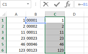
Note that the values are now displayed in numerical format.

Text splitting function in Excel

Individual functions and their combinations allow you to distribute words from one cell to separate cells:

LEFT (Text, number of characters) displays the specified number of characters from the beginning of the cell;
RIGHT (Text, number of characters) returns a specified number of characters from the end of the cell;
SEARCH (Search text, range to search, start position) shows the position of the first occurrence of the searched character or line while viewing from left to right.

The line takes into account the position of each character when dividing the text. Spaces show the beginning or the end of the name you are looking for.

We will split the name, surname and patronymic name into different columns using the functions.

split.

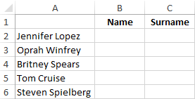
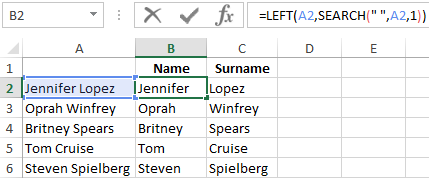
The first line contains only the first and last names separated by a space. Formula for retrieving the name:

The function SEARCH is used to determine the second argument of the LEFT function (the number of characters). It finds a space in cell A2 starting from the left.

For a name, we use the same formula:

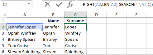
Excel determines the number of characters for the RIGHT function using the SEARCH function. The LEN function «counts» the total length of the text. Then the number of characters up to the first space (found by SEARCH) is subtracted.

The formula for extracting the surname:

Next formulas for extracting the surname is a bit different:

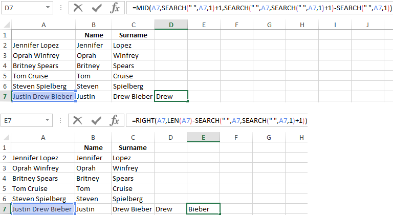
These are five signs on the right. Embedded SEARCH functions search for the second and third spaces in a string. SEARCH («»;A7;1) finds the first space on the left (before the patronymic name). Add one (+1) to the result. We get the position with which we will search for the second space.

Part of the formula SEARCH(» «;A7;SEARCH(» «;A7;1)+1) finds the second space. This will be the final position of the patronymic.

Then the number of characters from the beginning of the line to the second space is subtracted from the total length of the line. The result is the number of characters to the right that you need to return.

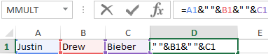
Function for merging text in Excel

Use the ampersand (&) operator or the CONCATENATE function to combine values from several cells into one line.

For example, the values are located in different columns (cells):

Put the cursor in the cell where the combined three values will be. Enter «=». Select the first cell and click on the keyboard «&» sign. Then enter the space character enclosed in quotation marks (» «). Enter again «&». Therefore, sequentially connect cells with symbols and spaces.

We get the combined values in one cell:

Using the CONCATENATE function:

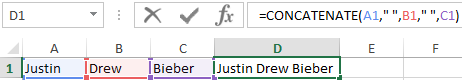
You can add any sign or string to the final expression using quotation marks in the formula.

Text SEARCH function in Excel

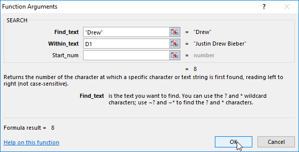
The SEARCH function returns the starting position of the searched text (not case sensitive). For example:

SEARCH.

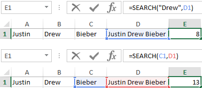
The SEARCH returned to position 8 because the word «Drew» begins with the tenth character in the line. Where can this be useful?

The SEARCH function determines the position of the character in the string line. And the MID function returns symbols values (see the example above). Alternatively, you can replace the found text with the REPLACE.

syntax.

Download example TEXT functions

The syntax of the SEARCH function:

«Find_text» is what you need to find;
«Withing_text» is where to look;
«Start_num» is from which position to start searching (by default it is 1).

Use the FIND if you need to take into account the case (lower and upper).

Источник

The TEXT excel function converts a number to a text string based on the format specified by the user. This format is supplied as an argument to the TEXT function. Since the resulting outputs are text representations of numbers, they cannot be used as is in formulas. Therefore, it is recommended to retain the original numbers and create a separate row or column for the converted numbers.

For example, the formula “=TEXT(“10/2/2022″,”mmmm dd, yyyy”)” returns February 10, 2022. Exclude the beginning and ending double quotation marks while entering this formula in Excel.

The purpose of using the TEXT function in Excel is to display a number in the desired format. Since this function also helps combine numbers with other text strings, it tends to make the output more legible. The TEXT function is particularly used when the number formats of different datasets need to be made identical.

Estimated reading time: 21 minutes

What is Text Function in Excel?
- Syntax of the TEXT Function of Excel
- How to Use the TEXT Function in Excel?
  - Example #1–Prefix the Text Strings to the Newly Formatted Date Values
  - Example #2–Join the Newly Formatted Time and Date Values
  - Example #3–Extract a Mobile Number from its Scientific Notation
  - Example #4–Prefix a Text String to the Initially Formatted Monetary Value
- Date Formats of Excel
- Frequently Asked Questions
- TEXT Function in Excel Video
- Recommended Articles

Syntax of the TEXT Function of Excel

The syntax of the TEXT function of Excel is shown in the following image:

The TEXT function of Excel accepts the following arguments:

Value: This is the number to be converted to a text string. Apart from a number, a date, time or cell reference can also be supplied to the TEXT excel function. The cell reference can contain either a number or an output of another function which can be a number or date.
Format_text: This is the format to be applied to the “value” argument. It is also called the format code. It is entered within double quotation marks in the TEXT formula of Excel. For instance, “0.00,” “dd/mm/yyyy,” “hh:mm:ss,” and so on are format codes.

Both the stated arguments are mandatory.

Note 1: The format code “0.00” displays a number with two decimal places. In the format code “dd/mm/yyyy,” “dd,” “mm,” and “yyyy” are the notations for days (in two digits), months (in two digits), and years (in four digits) respectively.

Likewise, “hh,” “mm,” and “ss” are the notations for hours (in two digits), minutes (in two digits), and seconds (in two digits) respectively.

For the meaning of the different date formats, refer to the heading “date formats of Excel” given after example #4 of this article.

Note 2: The TEXT function is categorized as a Text/String function of Excel. The TEXT function is available in all versions of Excel.

How to Use the TEXT Function in Excel?

Let us consider some examples to understand the working of the TEXT function in Excel.

Example #1–Prefix the Text Strings to the Newly Formatted Date Values

The following table shows the names of five children along with the dates they were born on. The dates are currently in the format m/d/yyyy. Consider the two columns and six rows of the table as columns A and B and rows 1 to 6 of Excel.

We want to perform the following tasks:

Join the name and date of birth of row 2 by using the ampersand operator. There should not be any space between the joined values.
Convert each date to the format “dd mmm, yyyy.” Prefix the child’s name and the string “was born on” to each date.
Show the output when the date of row 2 is in the format “d mmm, yyyy.” Let the prefixes of the preceding point stay as it is.
Show the date formats “dd mmm, yyyy” (in cell C2) and “d mmm, yyyy” (in cell C6) in a single column.

Explain the outputs obtained in the second and fourth bullet points. Use the TEXT function of Excel.

Name of Kid	Date of Birth
John	12/8/2015
Patricia	1/12/2014
Ram	3/11/2016
Anita	11/11/2017
Davis	5/6/2014

The steps to perform the given tasks by using the TEXT function of Excel are listed as follows:

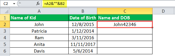
Step 1: Enter the following formula in cell C2. Exclude the beginning and ending double quotation marks while entering the given formula.

“=A2&“”&B2”

This formula (shown in the image of step 2) joins the values of cells A2 and B2 without any spaces in-between.

Note: The ampersand operator (&) helps join the values of two or more cells. It is called the concatenation operator and is used as an alternative to the CONCATENATE function of Excel. There is no limit on the number of cell values that the ampersand can join.

Step 2: Press the “Enter” key. The output appears in cell C2, as shown in the following image.

Notice that Excel has joined the values of cells A2 and B2 without any spaces in-between. However, the output is not in a readable format. The reason is that the date (12/8/2015) has been converted to a sequential number. The number 42346 represents the date December 8, 2015.

Note: A date is stored in Excel as a sequential or a serial number. This is because a serial number makes it easy to perform calculations. To view the serial number of a date, refer to the “note” preceding step 3 of example #2.

Step 3: To apply the format “dd mmm, yyyy” and insert the stated prefixes, enter the following formula in cell C2.

“=A2&” was born on “&TEXT(B2,”dd mmm, yyyy”)”

Press the “Enter” key. Then, drag the formula of cell C2 till cell C6 by using the fill handle. The outputs are displayed in the following image.

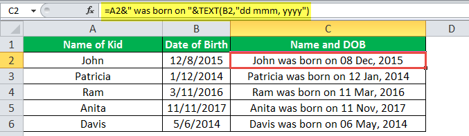
Explanation of the outputs: In column C of the preceding image, the child’s name (in column A) and the text string (was born on) have been prefixed to each date of column B. Since the date is in a suitable format, the output is readable now.

The joined values (outputs) of column C are in the form of statements that are easier to understand than the single values of columns A and B.

Notice that, to insert spaces as the separators in the output, we have inserted spaces at the relevant places in the formula of step 1. Moreover, a comma has also been inserted after the notation of months (mmm). This comma can be seen in each date of the output (in column C).

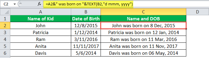
Step 4: To see the output when the date format is “d mmm, yyyy” and the prefixes are in place, enter the following formula in cell C2.

=A2&” was born on “&TEXT(B2,”d mmm, yyyy”)

Press the “Enter” key. The output appears in cell C2, as shown in the following image.

Notice that the leading zero before the date 8 Dec, 2015 (in cell C2) has disappeared. This zero was there in cell C2 of the preceding image. It has disappeared because, in the current format code, the number of days is represented by a single “d.”

A single “d” omits the leading zeros when the number of days is in a single digit.

Step 5: The outputs obtained after applying different date formats in the same column (column C) are shown in the following image.

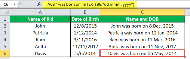
Explanation of the outputs: Notice that in the preceding image, the date of cell C2 is in the format “d mmm, yyyy” while that of cell C6 is in the format “dd mmm, yyyy.” The only difference between these two date formats is in the number of days. The leading zero is absent in cell C2 and present in cell C6.

Hence, with the TEXT function of Excel, one can have different date formats in different cells of the same column. Remember that a format code changes only the appearance of a value; it does not change the value itself. One can create a format code depending on the requirement.

Example #2–Join the Newly Formatted Time and Date Values

The following table shows the times and dates in two separate columns. Consider these columns as columns A and B of Excel. We want to perform the following tasks:

Join (concatenate) each time value with the respective date. Use the ampersand operator (&) and ensure that there is no space between the two values.
Show how to copy the formats “h:mm:ss am/pm” and “m/d/yyyy” from the “format cells” window. Convert each time to the former and date to the latter format.
Join the converted time and date values with the ampersand operator (&). Ensure that there is a space between the two values.
Show the output when the date format is not enclosed within double quotation marks.

Explain the outputs obtained in the first and third bullet points. Use the TEXT function of Excel for the given tasks.

Time	Date
7:00:00 AM	6/19/2018
7:15:00 AM	6/19/2018
7:30:00 AM	6/19/2018
7:45:00 AM	6/19/2018
8:00:00 AM	6/19/2018
8:15:00 AM	6/19/2018
8:30:00 AM	6/19/2018
8:45:00 AM	6/19/2018

The steps to perform the given tasks by using the TEXT function of Excel are listed as follows:

Step 1: Enter the following formula (without the beginning and ending double quotation marks) in cell C2.

“=A2&“”&B2”

This formula is shown in the image of step 2. It joins the values of cells A2 and B2 without a space in-between.

Step 2: Press the “Enter” key. Then, drag the formula of cell C2 till cell C9 by using the fill handle. The fill handle is displayed at the bottom-right side of cell C2.

The outputs are shown in the following image.

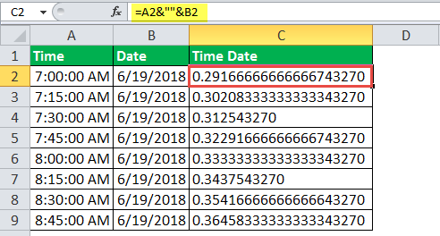
Explanation of the outputs: In column C, the number 43270 (at the end) is the same throughout the range C2:C9. This is the serial number for the date June 19, 2018. The entire decimal number preceding this serial number is the time. So, the decimal number 0.2916667 (in cell C2) represents the time 7:00:00 am.

The outputs obtained in column C of the preceding image are not readable. The reason is that Excel has converted the times (of column A) to decimal numbers and dates (of column B) to sequential numbers. Moreover, joining the decimals with sequential numbers has made the outputs more complicated.

To be able to read the output, it needs to be converted to the relevant format codes. This conversion is shown further in this example.

Note: Excel stores dates as sequential (or serial) numbers and times as decimal numbers. Excel considers a time value as a part of a day. To view the number representing the date, perform the following actions:

Select any cell of the range B2:B9.
Press the keys “Ctrl+1” together. The “format cellsFormatting cells is an important technique to master because it makes any data presentable, crisp, and in the user’s preferred format. The formatting of the cell depends upon the nature of the data present.read more” window opens.
Select “general” under “category” in the “number” tab.

The serial number can be seen under “sample.” Click “cancel” to close the “format cells” window or “Ok” to change the date to a serial number.

Likewise, the decimal number representing the time can also be seen by selecting any cell of the range A2:A9 and following actions “b” and “c” listed above.

Step 3: To convert the time and date values to a readable format, let us first copy the format codes from the “format cells” window. So, select cell C2 and press the keys “Ctrl+1” together.

The “format cells” window opens, as shown in the following image. From the “number” tab, select “custom” under “category. Excel provides a list of formats under “type.”

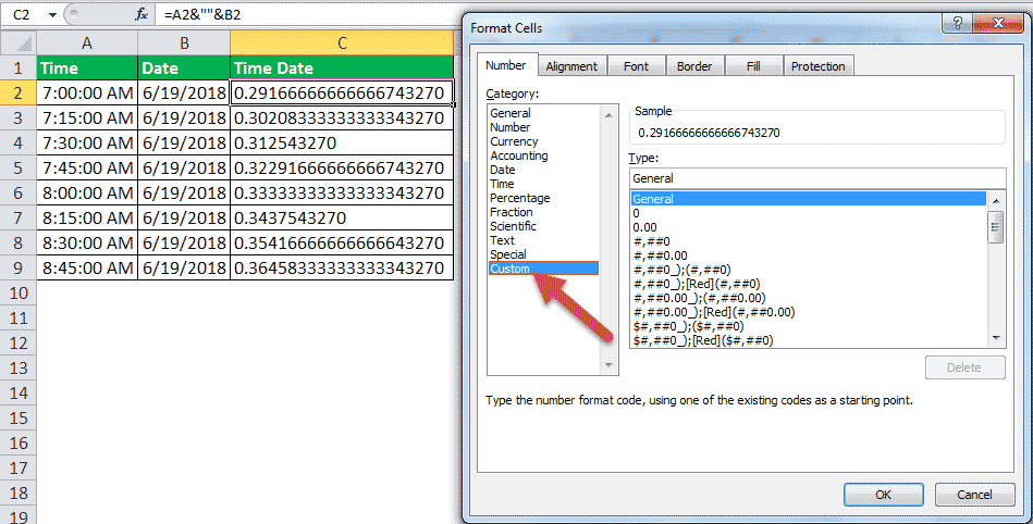
Step 4: Scroll down the list of formats given under “type.” Copy the format “h:mm:ss am/pm.” To copy, just select the format code and press the keys “Ctrl+C.”

The format code is shown in the following image. Once the format has been copied, close the “format cells” window.

Step 5: Copy the format code “m/d/yyyy” for converting the date values. This format code is also available under “type,” as shown in the following image.

Close the “format cells” window after copying the mentioned format code.

Step 6: To apply the new formats to the time and date values and join the resulting values, enter the following formula in cell C2.

“=TEXT(A2,”h:MM:SS AM/PM”)&” “&TEXT(B2,”m/d/yyyy”)”

This formula is shown in the image of step 7. If the format codes have been copied in the preceding steps, they can be pasted at the relevant places in the formula by pressing the shortcut “Ctrl+V.”

According to this formula, the time and date values of cells A2 and B2 are formatted as per the codes “h:MM:SS AM/PM” and “m/d/yyyy” respectively. The formatted (or converted) values are then joined with the ampersand operator.

Notice that in the formula, a space has also been entered within a pair of double quotation marks (like &“ ”&). This space will be inserted in the output at exactly that place where it has been entered in the formula.

Step 7: Press the “Enter” key after entering the TEXT formula. Drag the formula of cell C2 till cell C9.

The outputs are shown in the following image.

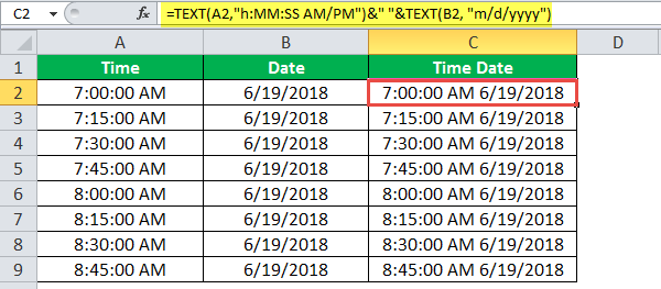
Explanation of the outputs: The time and date values of columns A and B have been converted to the relevant formats in column C. The time values display the hours (h) in a single digit, minutes (mm) in two digits, and seconds (ss) also in two digits. Since all the time values belong to the period before noon, they display “am” at the end.

Likewise, the dates display the months (m) in a single digit, days (d) in a single digit, and years (yyyy) in four digits.

Notice that there is a space between the two joined values in column C. Even though we copied the code “h:mm:ss am/pm” (in step 4) and pasted “h:MM:SS AM/PM” (in step 6), we obtained the correct outputs in column C (in step 7). This is because the format codes are not case-sensitive, implying that “mm” is treated the same as “MM.”

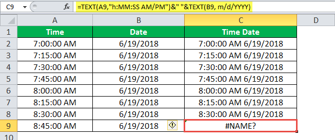
Step 8: To see what happens when the format code for date is entered without the double quotation marks, type the following formula in cell C9.

“=TEXT(A2,”h:MM:SS AM/PM”)&” “&TEXT(B2,m/d/YYYY)”

Press the “Enter” key. Excel returns the “#NAME?” error, as shown in the following image. Therefore, for the TEXT excel function to work, the format code should necessarily be enclosed within double quotation marks.

There are two images titled “image 1” and “image 2.” The following information is given:

Image 1 shows a number having eleven 9s in cell B2. When 1 is added to this number, its digits increase to 12. Excel displays the resulting 12-digit number (in cell B3) in a scientific notation.
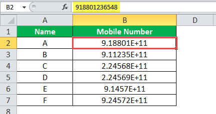
Image 2 shows the names of some people (in column A) and their random mobile numbers in a scientific notation (in column B). The formula bar shows the mobile number of person A. Each mobile number consists of twelve digits, which includes a 2-digit country code at the beginning.

Note that a scientific notationIn Excel, scientific notation is a specific style of writing numbers in scientific and exponential forms. Scientific notation compactly helps display values, allowing us to compare and use the same in calculations.read more (or scientific format) often displays very large or very small numbers in a contracted form. We want to perform the following tasks:

Display the entire 12-digit mobile number without any spaces in-between.
Separate the country code from the rest of the number with the help of a hyphen.

Use the TEXT function of Excel for the given tasks.

Image 1

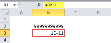
Image 2

The steps to perform the given tasks by using the TEXT function of Excel are listed as follows:

Step 1: Enter the following formula in cell D2.

“=TEXT(B2,”############”)”

This formula is shown in the formula bar of the succeeding image. Notice that there are 12 hashes in the formula, which represent the 12 digits of a mobile number.

Step 2: Press the “Enter” key. The output appears in cell D2. To obtain the outputs for the entire column D, drag the formula of cell D2 to cell D7. Use the fill handle of cell D2 (displayed at the bottom-right corner) for dragging.

The outputs of column D are shown in the succeeding image.

Note: The output is displayed (in column D) only when one enters a mobile number as an input (in column B) which is converted automatically (or manually) to a scientific format of Excel. In case, a scientific format is typed manually in column B; it cannot be converted to a mobile number of column D.

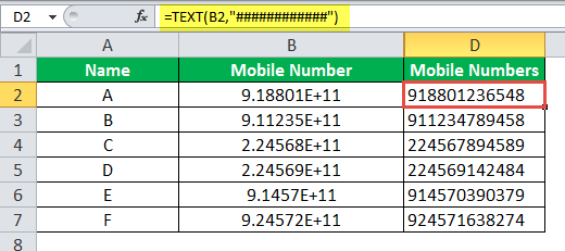
Step 3: To separate the country codes from the rest of the number by using a hyphen, enter the following formula in cell D2.

“=TEXT(B2,“##-##########”)”

Press the “Enter” key. Next, drag the formula of cell D2 till cell D7 with the help of the fill handle. The formula of cell D2 and the outputs are shown in the following image.

Notice that in the formula, the hyphen is placed exactly where it is required in the output. Since only the first two digits of each mobile number are to be separated, the hyphen is placed after two hashes of the formula.

Example #4–Prefix a Text String to the Initially Formatted Monetary Value

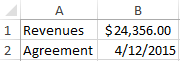
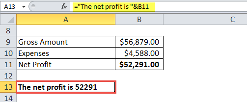
There are two images titled “image 1” and “image 2.” The following information is given:

Image 1 shows the gross profit, expenses, and net profit of an organization. All these numbers are in dollars.
Image 2 shows how the net profit has been computed. To calculate the net profit, the expenses have been subtracted from the gross profit.

We want to perform the following tasks:

Show the output when the string “the net profit is” is prefixed to the amount of net profit. Use the ampersand operator for this purpose.
Prefix the string “the net profit is” to the amount of net profit by using the ampersand. Ensure that in the output, the amount of net profit displays the dollar sign ($) and the comma at the correct places (like $52,291). Use the TEXT function of Excel for this purpose.

Explain the output obtained at the end.

Image 1

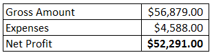
Image 2

The steps to perform the given tasks are listed as follows:

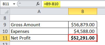
Step 1: Enter the following formula in cell A13.

“=”The net profit is “&B11”

Exclude the beginning and ending double quotation marks of the formula while entering it in Excel. This formula is shown in the image of step 2.

The given formula prefixes the string “the net profit is” to the value of cell B11. The ampersand helps join the stated string to the amount of net profit (in cell B11).

Step 2: Press the “Enter” key. The output appears in cell A13, as shown in the following image.

Notice that the dollar sign and the comma of the net profit amount (shown in cell B11) have been omitted in the output. Though the string “the net profit is” has been correctly prefixed. The spaces have also been inserted at the right places in cell A13.

Step 3: To retain the dollar sign and the comma of the amount, enter the following formula in cell A13.

“=”The net profit is ” &TEXT(B11,”$#,##0.00″)”

Press the “Enter” key. The formula and the output are shown in cell A13 of the following image.

Notice that by mistake, a space has been inserted before the ampersand in the formula. However, even then, the correct output has been obtained in cell A13.

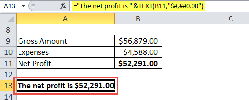
Explanation of the output: This time, the amount of net profit has been properly written (including the dollar sign and the comma) in cell A13. The reason is that the amount of net profit has been converted to the appropriate format in addition to being prefixed by a text string.

So, with the TEXT function of Excel, one can join a number with any string and, at the same time, retain the initial formatting of the number.

Date Formats of Excel

The different format codes for dates have been described as follows:

Frequently Asked Questions

1. Define the TEXT function in Excel with the help of an example.

The TEXT function in Excel helps convert a numerical value to a text string. The conversion is carried out according to the format specified by the user. Once converted, the numerical value becomes a text representation of a number.

The formula “=TEXT(“2/12/2021”,“dddd-mmmm-yyyy”)” converts the date 2/12/2021 to Thursday-December-2021. Ensure that the beginning and ending double quotation marks are excluded while entering this TEXT formula in Excel.

Note: For the working of the TEXT function of Excel, refer to the examples of this article.

2. Why is the TEXT function used in Excel?

The TEXT function is used in Excel for the following reasons:

• It helps convert a numerical value to a text string having a new format.
• It eases joining a numerical value with a text string.
• It helps retain the format of the existing numerical value after concatenation (joining).
• It makes the date or time values given in sequential or decimal numbers more readable and understandable for the users.
• It helps add the leading zeros to a number.
• It allows inserting specific characters (like +,-,(),<>,: etc.) in the output.

Note: The different characters that can be entered in the TEXT formula are the plus (+), minus (-), equal to (=), parentheses (), less than and greater than signs <>, colon (:), apostrophe (‘), curly braces {}, caret (^), forward slash (/), ampersand (&), space ( ), tilde (~), and an exclamation point (!).

The characters should be entered in the format code. These characters are displayed at exactly those places (in the output) where they have been entered in the format code.

3. How is the TEXT function used to add the leading zeros to a number in Excel?

The steps to add the leading zeros to a number are listed as follows:

a. Type “=TEXT” followed by the opening parenthesis.
b. Enter the number as the “value” argument.
c. Enter those many zeros in the format code as the number of digits required in the output.
d. Close the parenthesis and press the “Enter” key.

The leading zeros are added to the number entered in step “b.”

For instance, if the number 148 should appear as a 5-digit number, enter the formula “=TEXT(“148”,“00000”)” without the beginning and ending double quotation marks. It returns 00148.

Overview

Download our examples

Other format codes that are available

Format codes by category

Common scenario

Frequently Asked Questions

See Also

See Also

Need more help?

What is the Excel TEXT Function?

Formula

When is the Excel TEXT Function required?

Examples

1. Basic example – Excel Text Function

2. Using Excel TEXT with other functions

3. Combining the text given with data using TEXT function

4. Adding zeros before numbers with variable lengths

5. Converting telephone numbers to a specific format

Format Code

If the Excel TEXT function isn’t working

Tips

Free Excel Course

Additional Resources

Article Sources

Examples with TEXT function in Excel

Text splitting function in Excel

Function for merging text in Excel

Text SEARCH function in Excel

Table of contents

Syntax of the TEXT Function of Excel

How to Use the TEXT Function in Excel?

Example #1–Prefix the Text Strings to the Newly Formatted Date Values

Example #2–Join the Newly Formatted Time and Date Values

Example #4–Prefix a Text String to the Initially Formatted Monetary Value

Date Formats of Excel

Frequently Asked Questions

TEXT Function in Excel Video

Recommended Articles