
This tutorial explains what different symbols mean in formulas in Excel and Google Sheets.
Excel is essentially used for keeping track of data and using calculations to manipulate this data. All calculations in Excel are done by means of formulas, and all formulas are made up of different symbols or operators, depending on what function the formula is performing.
Equal Sign (=)
The most commonly used symbol in Excel is the equal (=) sign. Every single formula or function used has to start with equals to let Excel know that a formula is being used. If you wish to reference a cell in a formula, it has to have an equal sign before the cell address. Otherwise, Excel just shows the cell address as standard text.
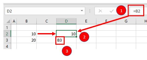
In the above example, if you type (1) =B2 in cell D2, it returns a value of (2) 10. However, typing only (3) B3 into cell D3 just shows “B3” in the cell, and there is no reference to the value 20.
Standard Operators
The next most common symbols in Excel are the standard operators as used on a calculator: plus (+), minus (–), multiply (*) and divide (/). Note that the multiplication sign is not the standard multiplication sign (x) but is depicted by an asterisk (*) while the division sign is not the standard division sign (÷) but is depicted by the forward slash (/).
An example of a formula using addition and multiplication is shown below:
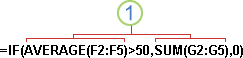
=B1+B2*B3Order of Operations and Adding Parentheses
In the formula shown above, B2*B3 is calculated first, as in standard mathematics. The order of operations is always multiplication before addition. However, you can adjust the order of operations by adding parentheses (round brackets) to the formula; any calculations between these parentheses would then be done first before the multiplication. Parentheses, therefore, are another example of symbols used in Excel.
=(B1+B2)*B3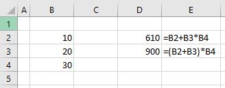
In the example shown above, the first formula returns a value of 610 while the second formula (using parentheses) returns 900.
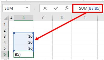
Parentheses are also used with all Excel functions. For example, to sum B3, B4, and B5 together, you can use the SUM Function where the range B3:B5 is contained within parentheses.
=SUM(B3:B5)Colon (:) to Specify a Range of Cells
In the formula used above, the parentheses contain the cell range which the SUM Function needs to add together. This cell range is expressed with a colon (:) where the first cell reference (B3) is the cell address of the first cell included in the range of cells to add together, while the second cell reference (B5) is the cell address of the last cell included in the range.
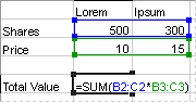
Dollar Symbol ($) in an Absolute Reference
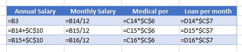
A particular useful and common symbol used in Excel is the dollar sign within a formula. Note that this does not indicate currency; rather, it’s used to “fix” a cell address in place in order that a single cell can be used repetitively in multiple formulas by copying formulas between cells.
=C6*$C$3By adding a dollar sign ($) in front of the column header (C) and the row header (3), when copying the formula down to Rows 7–15 in the example below, the first part of the formula (e.g., C6) changes according to the row it is copied down to while the second part of the formula ($C$3) stays static always enabling the formula to refer to the value stored in cell C3.
See: Cell References and Absolute Cell Reference Shortcut for more information on absolute references.
Exclamation Point (!) to Indicate a Sheet Name
The exclamation point (!) is critical if you want to create a formula in a sheet and include a reference to a different sheet.
=SUM(Sheet1!B2:B4)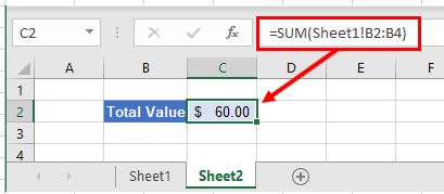
Square Brackets [ ] to Refer to External Workbooks
Excel uses square brackets to show references to linked workbooks. The name of the external workbook is enclosed in square brackets, while the sheet name in that workbook appears after the brackets with an exclamation point at the end.
Comma (,)
The comma has two uses in Excel.
Refer to Multiple Ranges
If you wish to use multiple ranges in a function (e.g., the SUM Function), you can use a comma to separate the ranges.
=SUM(B2:B3, B6:B10)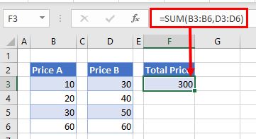
Separate Arguments in a Function
Alternatively, some built in Excel functions have multiple arguments which are usually separated with commas. (These can also be semicolons, depending on the function syntax.)
=VLOOKUP(H5, B6:E15, 4, FALSE)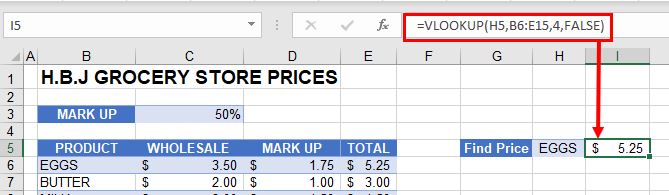
Curly Brackets { } in Array Formulas
Curly brackets are used in array formulas. An array formula is created by pressing the CTRL + SHIFT + ENTER keys together when entering a formula.
Other Important Symbols
| Symbol | Description | Example |
|---|---|---|
| % | Percentage | =B2% |
| ^ | Exponential operator | =B2^B3 |
| & | Concatenation | =B2&B3 |
| > | Greater than | =B2>B3 |
| < | Less than | =B2<B3 |
| >= | Greater than or equal to | =B2>=B3 |
| <= | Less than or equal to | =B2<=B3 |
| <> | Not equal to | =B2<>B3 |
Symbols in Formulas in Google Sheets
The symbols used in Google Sheets are identical to those used in Excel.
Symbols used in Excel Formula
| Symbol | Name |
|---|---|
| () | Parentheses |
| * | Asterisk |
| , | Comma |
| & | Ampersand |
Contents
- 1 What are the symbols in Excel formulas?
- 2 What does ‘@’ mean in Excel formula?
- 3 What symbol do all formulas in Excel start with?
- 4 What does ‘!’ Mean in Excel formula?
- 5 Where are Symbols in Excel?
- 6 How do you sum symbols in Excel?
- 7 What does the exclamation mark mean in Excel?
- 8 What does semicolon mean in Excel formula?
- 9 What symbol means?
- 10 What do you mean by symbol and formula?
- 11 What is a symbol called?
- 12 Why are symbols used?
- 13 How do you use symbols?
- 14 What is Sigma in Excel?
- 15 How do you use PI in Excel?
- 16 How columns are Labelled in Excel?
- 17 What does the symbol ∧ mean?
- 18 What are the algebra symbols?
- 19 What is the symbol for mean in stats?
- 20 What does the icon exclamation mark mean?
Using arithmetic operators in Excel formulas
| Operator | Meaning | Formula example |
|---|---|---|
| * (asterisk) | Multiplication | =A2*B2 |
| / (forward slash) | Division | =A2/B2 |
| % (percent sign) | Percentage | =A2*10% (returns 10% of the value in A2) |
| ^ (caret) | Exponential (power of) | =A2^3 (raises the number in A2 to the power of 3) |
What does ‘@’ mean in Excel formula?
The @ symbol is already used in table references to indicate implicit intersection. Consider the following formula in a table =[@Column1]. Here the @ indicates that the formula should use implicit intersection to retrieve the value on the same row from [Column1].
What symbol do all formulas in Excel start with?
equal sign (=)
A formula always begins with an equal sign (=). Excel for the web interprets the characters that follow the equal sign as a formula. Following the equal sign are the elements to be calculated (the operands), such as constants or cell references. These are separated by calculation operators.
What does ‘!’ Mean in Excel formula?
When entered as the reference of a Named range , it refers to range on the sheet the named range is used on. For example, create a named range MyName refering to =SUM(!B1:!K1) Place a formula on Sheet1 =MyName . This will sum Sheet1! B1:K1.
Where are Symbols in Excel?
Insert tab
Click the Insert tab and then click the Symbol button in the Symbols group. The Symbol dialog box appears. The Symbol dialog box contains two tabs: Symbols and Special Characters.
How do you sum symbols in Excel?
To use a shortcut instead, hold down the Alt key, then type ALT+2+2+8 (Alt 228) to insert the sum (Σ) symbol.
What does the exclamation mark mean in Excel?
The exclamation mark means that the workbook is a macro-enabled workbook with extension . xlsm (a standard Excel 2007/2010 workbook cannot contain macros and has extension .
What does semicolon mean in Excel formula?
In Microsoft Excel, the semicolon is used as a list separator, especially in cases where the decimal separator is a comma, such as 0,32; 3,14; 4,50 , instead of 0.32, 3.14, 4.50 .
What symbol means?
1 : something that stands for something else : emblem The eagle is a symbol of the United States. 2 : a letter, character, or sign used instead of a word to represent a quantity, position, relationship, direction, or something to be done The sign + is the symbol for addition.
What do you mean by symbol and formula?
A chemical symbol is a one- or two-letter designation of an element.Compounds are combinations of two or more elements. A chemical formula is an expression that shows the elements in a compound and the relative proportions of those elements.
What is a symbol called?
This table contains special characters.
| Symbol | Name of the symbol | Similar glyphs or concepts |
|---|---|---|
| ≈ | Almost equal to | Equals sign |
| & | Ampersand | |
| ⟨ ⟩ | Angle brackets | Bracket, Parenthesis, Greater-than sign, Less-than sign |
| ‘ ‘ | Apostrophe | Quotation mark, Guillemet, Prime |
Why are symbols used?
Human cultures use symbols to express specific ideologies and social structures and to represent aspects of their specific culture. Thus, symbols carry meanings that depend upon one’s cultural background; in other words, the meaning of a symbol is not inherent in the symbol itself but is culturally learned.
How do you use symbols?
Go to Insert > Symbol. Pick a symbol, or choose More Symbols. Scroll up or down to find the symbol you want to insert. Different font sets often have different symbols in them and the most commonly used symbols are in the Segoe UI Symbol font set.
What is Sigma in Excel?
Sigma is a Greek letter that appears just like the Latin letter M on its side! That, ∑ In mathematics and statistics sigma, ∑, means that sum of, to add along. The sigma operate in excel, therefore, is add (values)
How do you use PI in Excel?
Excel Character Code for Pi
To add the pi symbol to a cell this way, hold down the ALT Key and type 227 on the number pad. Then release the ALT key, and the symbol, or Greek letter, “π” will be inserted in the cell.
How columns are Labelled in Excel?
By default, Excel uses the A1 reference style, which refers to columns as letters (A through IV, for a total of 256 columns), and refers to rows as numbers (1 through 65,536). These letters and numbers are called row and column headings. To refer to a cell, type the column letter followed by the row number.
What does the symbol ∧ mean?
Wedge (∧) is a symbol that looks similar to an in-line caret (^). It is used to represent various operations.Some authors who call the descending wedge vel often call the ascending wedge ac (the corresponding Latin word for “and”, also spelled “atque”), keeping their usage parallel!
What are the algebra symbols?
Algebra Symbols With Names
| Symbol | Symbol Name | Meaning/definition |
|---|---|---|
| := | equal by definition | equal by definition |
| ≜ | equal by definition | equal by definition |
| ≈ | approximately equal | approximation |
| ~ | approximately equal | weak approximation |
What is the symbol for mean in stats?
The symbol ‘μ‘ represents the population mean.The symbol ‘N’ represents the total number of individuals or cases in the population.
What does the icon exclamation mark mean?
This symbol indicates that hazardous products with this pictogram can cause certain health effects for example, skin irritation, eye irritation, and/or.
Содержание
- What Do the Symbols (&,$,<, etc.) Mean in Formulas? – Excel & Google Sheets
- Equal Sign (=)
- Standard Operators
- Order of Operations and Adding Parentheses
- Colon (:) to Specify a Range of Cells
- Dollar Symbol ($) in an Absolute Reference
- Exclamation Point (!) to Indicate a Sheet Name
- Square Brackets [ ] to Refer to External Workbooks
- Comma (,)
- Refer to Multiple Ranges
- Separate Arguments in a Function
- Curly Brackets in Array Formulas
- Other Important Symbols
- Symbols in Formulas in Google Sheets
- List of Symbols in Excel Formula (and Their Meanings)
- List of Symbols in Excel Formula and Their Meanings
- How to Use the Symbols
- Additional Note
- Overview of formulas in Excel
- Create a formula that refers to values in other cells
- See a formula
- Enter a formula that contains a built-in function
- Download our Formulas tutorial workbook
- Formulas in-depth
- Need more help?
What Do the Symbols (&,$,<, etc.) Mean in Formulas? – Excel & Google Sheets
This tutorial explains what different symbols mean in formulas in Excel and Google Sheets.
Excel is essentially used for keeping track of data and using calculations to manipulate this data. All calculations in Excel are done by means of formulas, and all formulas are made up of different symbols or operators, depending on what function the formula is performing.
Equal Sign (=)
The most commonly used symbol in Excel is the equal (=) sign. Every single formula or function used has to start with equals to let Excel know that a formula is being used. If you wish to reference a cell in a formula, it has to have an equal sign before the cell address. Otherwise, Excel just shows the cell address as standard text.
In the above example, if you type (1) =B2 in cell D2, it returns a value of (2) 10. However, typing only (3) B3 into cell D3 just shows “B3” in the cell, and there is no reference to the value 20.
Standard Operators
The next most common symbols in Excel are the standard operators as used on a calculator: plus (+), minus (–), multiply (*) and divide (/). Note that the multiplication sign is not the standard multiplication sign (x) but is depicted by an asterisk (*) while the division sign is not the standard division sign (÷) but is depicted by the forward slash (/).
An example of a formula using addition and multiplication is shown below:
Order of Operations and Adding Parentheses
In the formula shown above, B2*B3 is calculated first, as in standard mathematics. The order of operations is always multiplication before addition. However, you can adjust the order of operations by adding parentheses (round brackets) to the formula; any calculations between these parentheses would then be done first before the multiplication. Parentheses, therefore, are another example of symbols used in Excel.
In the example shown above, the first formula returns a value of 610 while the second formula (using parentheses) returns 900.
Parentheses are also used with all Excel functions. For example, to sum B3, B4, and B5 together, you can use the SUM Function where the range B3:B5 is contained within parentheses.
Colon (:) to Specify a Range of Cells
In the formula used above, the parentheses contain the cell range which the SUM Function needs to add together. This cell range is expressed with a colon (:) where the first cell reference (B3) is the cell address of the first cell included in the range of cells to add together, while the second cell reference (B5) is the cell address of the last cell included in the range.
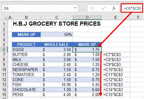
Dollar Symbol ($) in an Absolute Reference
A particular useful and common symbol used in Excel is the dollar sign within a formula. Note that this does not indicate currency; rather, it’s used to “fix” a cell address in place in order that a single cell can be used repetitively in multiple formulas by copying formulas between cells.
By adding a dollar sign ($) in front of the column header (C) and the row header (3), when copying the formula down to Rows 7–15 in the example below, the first part of the formula (e.g., C6) changes according to the row it is copied down to while the second part of the formula ($C$3) stays static always enabling the formula to refer to the value stored in cell C3.
See: Cell References and Absolute Cell Reference Shortcut for more information on absolute references.
Exclamation Point (!) to Indicate a Sheet Name
The exclamation point (!) is critical if you want to create a formula in a sheet and include a reference to a different sheet.
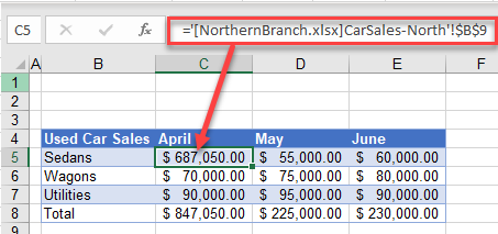
Square Brackets [ ] to Refer to External Workbooks
Excel uses square brackets to show references to linked workbooks. The name of the external workbook is enclosed in square brackets, while the sheet name in that workbook appears after the brackets with an exclamation point at the end.
Comma (,)
The comma has two uses in Excel.
Refer to Multiple Ranges
If you wish to use multiple ranges in a function (e.g., the SUM Function), you can use a comma to separate the ranges.
Separate Arguments in a Function
Alternatively, some built in Excel functions have multiple arguments which are usually separated with commas. (These can also be semicolons, depending on the function syntax.)
Curly Brackets in Array Formulas
Curly brackets are used in array formulas. An array formula is created by pressing the CTRL + SHIFT + ENTER keys together when entering a formula.
Other Important Symbols
| Symbol | Description | Example |
|---|---|---|
| % | Percentage | =B2% |
| ^ | Exponential operator | =B2^B3 |
| & | Concatenation | =B2&B3 |
| > | Greater than | =B2>B3 |
| = | Greater than or equal to | =B2>=B3 |
| Not equal to | =B2<>B3 |
Symbols in Formulas in Google Sheets
The symbols used in Google Sheets are identical to those used in Excel.
Источник
List of Symbols in Excel Formula (and Their Meanings)


In this tutorial, you will learn about the list of symbols in the excel formula that you can use.
There are many symbols you can use when you try to write a formula in excel. Each of them has its unique functions and you most probably need more than one symbol to complete your writing.
By knowing what are they and their functions, you should be better equipped to process data in excel using formulas. Therefore, master the excel formulas symbols by learning them from the list in this tutorial!
Disclaimer: This post may contain affiliate links from which we earn commission from qualifying purchases/actions at no additional cost for you. Learn more
Want to work faster and easier in Excel? Install and use Excel add-ins! Read this article to know the best Excel add-ins to use according to us!
List of Symbols in Excel Formula and Their Meanings
Here is a table that lists the symbols you can use in an excel formula. Each symbol is explained with its name, meaning, and formula writing example to help you understand them better.
| Symbol | Name | Meaning | Formula Writing Example |
|---|---|---|---|
| = | Equal | Marks the beginning of a formula writing | =A1 |
| Represents “equal to/the same as” in a logic condition | =A1=1 | ||
| + | Plus | Adds the number on the left with the number on the right | =2+3 |
| — | Minus | Subtracts the number on the left with the number on the right | =7-1 |
| * | Asterisk | Multiplies the number on the left with the number on the right | =3*8 |
| Represents a wildcard operator in criteria writing (any character in any amount) | =COUNTIF( A2:A101, ”Jim*” ) | ||
| / | Slash | Divides the number on the left with the number on the right | =10/2 |
| ^ | Caret | Powers the number on the left with the level of the number on the right | =3^2 |
| % | Percentage | Makes the number on its left side a percentage | =100*10% |
| More than | Represents “more than” in a logic condition | =IF( A1>8,”More than 8”,”Maximum 8” ) | |
| $ | Dollar | Make the row number or column letter on its right an absolute reference (won’t move when we copy the formula to other cells) | =$B$1+A6 |
| & | Ampersand | Concatenate the data on the left with the data on the right | =A2&B2&C2 |
| ? | Question | Represents a wildcard operator in criteria writing (any one character) | =COUNTIF( A2:A101, ”Jack?” ) |
| Tilde | Makes the * or ? symbol literal in criteria writing | =COUNTIF( A2:A101, ”Jack
*” ) |
|
| , | Comma | Separates one input and another (can be replaced by semicolon, depending on the excel settings) | =SUM( 1,3,8 ) |
| ; | Semicolon | Separates one input and another (can be replaced by comma, depending on the excel settings) | =SUM( 1;3;8 ) |
| : | Colon | Represents “to” in a cell range writing (A1:B10 means A1 to B10 cell in the cell range) | =SUM( A2:C2 ) |
| «» | Quotations | Becomes a media to type a text input directly in a formula | =IF( A2>70, «Pass», ”Fail” ) |
| » | Apostrophes | Becomes a media to input a workbook and worksheet name reference if the name has spaces | =вЂSheet1’!A1+A2 |
| ! | Exclamation | Separates a sheet name reference with the cell/cell range coordinate reference | =SUM( вЂSheet1’!A2:C2 ) |
| ( ) | Brackets | Becomes a media to give your formula inputs | =SUM( C2:C26 ) |
| Separates a certain calculation so it can run first | =2*(5+3) | ||
| Curly brackets | Represents an array formula (a formula that produces an array result) | ||
| [ ] | Square brackets | Becomes a media to input a field name of a table | =SUM( SalesData [Quantity] ) |
If a symbol has two meanings, then its actual meaning in your formula depends on the formula writing that you do.
How to Use the Symbols
To use the symbols you want, just begin typing a formula in one of your cells
Don’t forget to place an equal symbol (=) at the beginning of your formula writing. If you forget, then the symbols you type will become literal symbols.
Additional Note
Need to learn how to write a criterion with its symbols in a formula like COUNTIF or SUMIF? Check out this excel criterion writing guide in our COUNTIF tutorial if you need to. You should write them correctly so you won’t get a wrong result from your formula.
Other tutorials you should learn:
Источник
Overview of formulas in Excel
Get started on how to create formulas and use built-in functions to perform calculations and solve problems.

Important: The calculated results of formulas and some Excel worksheet functions may differ slightly between a Windows PC using x86 or x86-64 architecture and a Windows RT PC using ARM architecture. Learn more about the differences.
Important: In this article we discuss XLOOKUP and VLOOKUP, which are similar. Try using the new XLOOKUP function, an improved version of VLOOKUP that works in any direction and returns exact matches by default, making it easier and more convenient to use than its predecessor.
Create a formula that refers to values in other cells
Type the equal sign =.
Note: Formulas in Excel always begin with the equal sign.
Select a cell or type its address in the selected cell.

Enter an operator. For example, – for subtraction.
Select the next cell, or type its address in the selected cell.

Press Enter. The result of the calculation appears in the cell with the formula.
See a formula
When a formula is entered into a cell, it also appears in the Formula bar.

To see a formula, select a cell, and it will appear in the formula bar.

Enter a formula that contains a built-in function
Select an empty cell.
Type an equal sign = and then type a function. For example, =SUM for getting the total sales.
Type an opening parenthesis (.
Select the range of cells, and then type a closing parenthesis).

Press Enter to get the result.
Download our Formulas tutorial workbook
We’ve put together a Get started with Formulas workbook that you can download. If you’re new to Excel, or even if you have some experience with it, you can walk through Excel’s most common formulas in this tour. With real-world examples and helpful visuals, you’ll be able to Sum, Count, Average, and Vlookup like a pro.
Formulas in-depth
You can browse through the individual sections below to learn more about specific formula elements.
A formula can also contain any or all of the following: functions, references, operators, and constants.
Parts of a formula

1. Functions: The PI() function returns the value of pi: 3.142.
2. References: A2 returns the value in cell A2.
3. Constants: Numbers or text values entered directly into a formula, such as 2.
4. Operators: The ^ (caret) operator raises a number to a power, and the * (asterisk) operator multiplies numbers.
A constant is a value that is not calculated; it always stays the same. For example, the date 10/9/2008, the number 210, and the text «Quarterly Earnings» are all constants. An expression or a value resulting from an expression is not a constant. If you use constants in a formula instead of references to cells (for example, =30+70+110), the result changes only if you modify the formula. In general, it’s best to place constants in individual cells where they can be easily changed if needed, then reference those cells in formulas.
A reference identifies a cell or a range of cells on a worksheet, and tells Excel where to look for the values or data you want to use in a formula. You can use references to use data contained in different parts of a worksheet in one formula or use the value from one cell in several formulas. You can also refer to cells on other sheets in the same workbook, and to other workbooks. References to cells in other workbooks are called links or external references.
The A1 reference style
By default, Excel uses the A1 reference style, which refers to columns with letters (A through XFD, for a total of 16,384 columns) and refers to rows with numbers (1 through 1,048,576). These letters and numbers are called row and column headings. To refer to a cell, enter the column letter followed by the row number. For example, B2 refers to the cell at the intersection of column B and row 2.
The cell in column A and row 10
The range of cells in column A and rows 10 through 20
The range of cells in row 15 and columns B through E
All cells in row 5
All cells in rows 5 through 10
All cells in column H
All cells in columns H through J
The range of cells in columns A through E and rows 10 through 20
Making a reference to a cell or a range of cells on another worksheet in the same workbook
In the following example, the AVERAGE function calculates the average value for the range B1:B10 on the worksheet named Marketing in the same workbook.

1. Refers to the worksheet named Marketing
2. Refers to the range of cells from B1 to B10
3. The exclamation point (!) Separates the worksheet reference from the cell range reference
Note: If the referenced worksheet has spaces or numbers in it, then you need to add apostrophes (‘) before and after the worksheet name, like =’123′!A1 or =’January Revenue’!A1.
The difference between absolute, relative and mixed references
Relative references A relative cell reference in a formula, such as A1, is based on the relative position of the cell that contains the formula and the cell the reference refers to. If the position of the cell that contains the formula changes, the reference is changed. If you copy or fill the formula across rows or down columns, the reference automatically adjusts. By default, new formulas use relative references. For example, if you copy or fill a relative reference in cell B2 to cell B3, it automatically adjusts from =A1 to =A2.
Copied formula with relative reference

Absolute references An absolute cell reference in a formula, such as $A$1, always refer to a cell in a specific location. If the position of the cell that contains the formula changes, the absolute reference remains the same. If you copy or fill the formula across rows or down columns, the absolute reference does not adjust. By default, new formulas use relative references, so you may need to switch them to absolute references. For example, if you copy or fill an absolute reference in cell B2 to cell B3, it stays the same in both cells: =$A$1.
Copied formula with absolute reference

Mixed references A mixed reference has either an absolute column and relative row, or absolute row and relative column. An absolute column reference takes the form $A1, $B1, and so on. An absolute row reference takes the form A$1, B$1, and so on. If the position of the cell that contains the formula changes, the relative reference is changed, and the absolute reference does not change. If you copy or fill the formula across rows or down columns, the relative reference automatically adjusts, and the absolute reference does not adjust. For example, if you copy or fill a mixed reference from cell A2 to B3, it adjusts from =A$1 to =B$1.
Copied formula with mixed reference

The 3-D reference style
Conveniently referencing multiple worksheets If you want to analyze data in the same cell or range of cells on multiple worksheets within a workbook, use a 3-D reference. A 3-D reference includes the cell or range reference, preceded by a range of worksheet names. Excel uses any worksheets stored between the starting and ending names of the reference. For example, =SUM(Sheet2:Sheet13!B5) adds all the values contained in cell B5 on all the worksheets between and including Sheet 2 and Sheet 13.
You can use 3-D references to refer to cells on other sheets, to define names, and to create formulas by using the following functions: SUM, AVERAGE, AVERAGEA, COUNT, COUNTA, MAX, MAXA, MIN, MINA, PRODUCT, STDEV.P, STDEV.S, STDEVA, STDEVPA, VAR.P, VAR.S, VARA, and VARPA.
3-D references cannot be used in array formulas.
3-D references cannot be used with the intersection operator (a single space) or in formulas that use implicit intersection.
What occurs when you move, copy, insert, or delete worksheets The following examples explain what happens when you move, copy, insert, or delete worksheets that are included in a 3-D reference. The examples use the formula =SUM(Sheet2:Sheet6!A2:A5) to add cells A2 through A5 on worksheets 2 through 6.
Insert or copy If you insert or copy sheets between Sheet2 and Sheet6 (the endpoints in this example), Excel includes all values in cells A2 through A5 from the added sheets in the calculations.
Delete If you delete sheets between Sheet2 and Sheet6, Excel removes their values from the calculation.
Move If you move sheets from between Sheet2 and Sheet6 to a location outside the referenced sheet range, Excel removes their values from the calculation.
Move an endpoint If you move Sheet2 or Sheet6 to another location in the same workbook, Excel adjusts the calculation to accommodate the new range of sheets between them.
Delete an endpoint If you delete Sheet2 or Sheet6, Excel adjusts the calculation to accommodate the range of sheets between them.
The R1C1 reference style
You can also use a reference style where both the rows and the columns on the worksheet are numbered. The R1C1 reference style is useful for computing row and column positions in macros. In the R1C1 style, Excel indicates the location of a cell with an «R» followed by a row number and a «C» followed by a column number.
A relative reference to the cell two rows up and in the same column
A relative reference to the cell two rows down and two columns to the right
An absolute reference to the cell in the second row and in the second column
A relative reference to the entire row above the active cell
An absolute reference to the current row
When you record a macro, Excel records some commands by using the R1C1 reference style. For example, if you record a command, such as clicking the AutoSum button to insert a formula that adds a range of cells, Excel records the formula by using R1C1 style, not A1 style, references.
You can turn the R1C1 reference style on or off by setting or clearing the R1C1 reference style check box under the Working with formulas section in the Formulas category of the Options dialog box. To display this dialog box, click the File tab.
Need more help?
You can always ask an expert in the Excel Tech Community or get support in the Answers community.
Источник
![]()
Symbols Used in Excel Formula

Here are the important symbols used in Excel Formulas. Each of these special characters have used for different purpose in Excel. Let us see complete list of symbols used in Excel Formulas, its meaning and uses.
Symbols used in Excel Formula
Following symbols are used in Excel Formula. They will perform different actions in Excel Formulas and Functions.
| Symbol | Name | Description |
|---|---|---|
| = | Equal to | Every Excel Formula begins with Equal to symbol (=).
Example:=A1+A5 |
| () | Parentheses | All Arguments of the Excel Functions specified between the Parentheses.
Example:=COUNTIF(A1:A5,5) |
| () | Parentheses | Expressions specified in the Parentheses will be evaluated first. Parentheses changes the order of the evaluation in Excel Formula.
Example: =25+(35*2)+5 |
| * | Asterisk | Wild card operator to to denote all values in a List.
Example: =COUNTIF(A1:A5,”*“) |
| , | Comma | List of the Arguments of a Function Separated by Comma in Excel Formula.
Example: =COUNTIF(A1:A5,“>” &B1) |
| & | Ampersand | Concatenate Operator to connect two strings into one in Excel Formula.
Example: =”Total: “&SUM(B2:B25) |
| $ | Dollar | Makes Cell Reference as Absolute in Excel Formula.
Example:=SUM($B$2:$B$25) |
| ! | Exclamation | Sheet Names and Table Names Followed by ! Symbol in Excel Formula.
Example: =SUM(Sheet2!B2:B25) |
| [] | Square Brackets | Uses to refer the Field Name of the Table (List Object) in Excel Formula.
Example:=SUM(Table1[Column1]) |
| {} | Curly Brackets | Denote the Array formula in Excel.
Example: {=MAX(A1:A5-G1:G5)} |
| : | Colon | Creates references to all cells between two references.
Example: =SUM(B2:B25) |
| , | Comma | Union Operator will combine the multiple references into One.
Example: =SUM(A2:A25, B2:B25) |
| (space) | Space | Intersection Operator will create common reference of two references.
Example: =SUM(A2:A10 A5:A25) |
Share This Story, Choose Your Platform!
6 Comments
-
Redjen
May 31, 2022 at 12:37 pm — Replywhat is the symbol of average in excel?
-
PNRao
June 20, 2022 at 12:40 pm — ReplyYou can use AVERAGE()Function to calculate Average in Excel. If you wants to show the Average Statistical Symbol (x-bar), You can insert from symbols. F7C2 is the Unicode Hexa character for X-bar symbol. Make sure that you have set the Symbol Font :MS Reference Sans Serif.
-
-
Tom Pearce
September 22, 2022 at 3:54 pm — ReplyI have a workbook, where the original author used an @ sign in front of a function call in a formula. I can find no reference as to what the @ does, or how it is used. Any one know??
VBA Example: ActiveSheet.Range(“L2”).Formula = “=@CATEGORY($E2,LFC_AreaLU)”
Note: Category is a User Defined Function in the workbook.-
PNRao
December 5, 2022 at 11:30 am — Reply
-
-
Jane Girard
February 9, 2023 at 8:53 pm — ReplyI have this formula, do you know what the al means in the formula ?
IF(E4=””,””,VLOOKUP(C4,al,5,0)*E4), can-
PNRao
February 27, 2023 at 3:10 am — ReplyIt could be a defined Name or a name of the Table (List Object)
-
© Copyright 2012 – 2020 | Excelx.com | All Rights Reserved
Page load link
If you’re new to Excel for the web, you’ll soon find that it’s more than just a grid in which you enter numbers in columns or rows. Yes, you can use Excel for the web to find totals for a column or row of numbers, but you can also calculate a mortgage payment, solve math or engineering problems, or find a best case scenario based on variable numbers that you plug in.
Excel for the web does this by using formulas in cells. A formula performs calculations or other actions on the data in your worksheet. A formula always starts with an equal sign (=), which can be followed by numbers, math operators (such as a plus or minus sign), and functions, which can really expand the power of a formula.
For example, the following formula multiplies 2 by 3 and then adds 5 to that result to come up with the answer, 11.
=2*3+5
This next formula uses the PMT function to calculate a mortgage payment ($1,073.64), which is based on a 5 percent interest rate (5% divided by 12 months equals the monthly interest rate) over a 30-year period (360 months) for a $200,000 loan:
=PMT(0.05/12,360,200000)
Here are some additional examples of formulas that you can enter in a worksheet.
-
=A1+A2+A3 Adds the values in cells A1, A2, and A3.
-
=SQRT(A1) Uses the SQRT function to return the square root of the value in A1.
-
=TODAY() Returns the current date.
-
=UPPER(«hello») Converts the text «hello» to «HELLO» by using the UPPER worksheet function.
-
=IF(A1>0) Tests the cell A1 to determine if it contains a value greater than 0.
The parts of a formula
A formula can also contain any or all of the following: functions, references, operators, and constants.
1. Functions: The PI() function returns the value of pi: 3.142…
2. References: A2 returns the value in cell A2.
3. Constants: Numbers or text values entered directly into a formula, such as 2.
4. Operators: The ^ (caret) operator raises a number to a power, and the * (asterisk) operator multiplies numbers.
Using constants in formulas
A constant is a value that is not calculated; it always stays the same. For example, the date 10/9/2008, the number 210, and the text «Quarterly Earnings» are all constants. An expression or a value resulting from an expression is not a constant. If you use constants in a formula instead of references to cells (for example, =30+70+110), the result changes only if you modify the formula.
Using calculation operators in formulas
Operators specify the type of calculation that you want to perform on the elements of a formula. There is a default order in which calculations occur (this follows general mathematical rules), but you can change this order by using parentheses.
Types of operators
There are four different types of calculation operators: arithmetic, comparison, text concatenation, and reference.
Arithmetic operators
To perform basic mathematical operations, such as addition, subtraction, multiplication, or division; combine numbers; and produce numeric results, use the following arithmetic operators.
|
Arithmetic operator |
Meaning |
Example |
|
+ (plus sign) |
Addition |
3+3 |
|
– (minus sign) |
Subtraction |
3–1 |
|
* (asterisk) |
Multiplication |
3*3 |
|
/ (forward slash) |
Division |
3/3 |
|
% (percent sign) |
Percent |
20% |
|
^ (caret) |
Exponentiation |
3^2 |
Comparison operators
You can compare two values with the following operators. When two values are compared by using these operators, the result is a logical value — either TRUE or FALSE.
|
Comparison operator |
Meaning |
Example |
|
= (equal sign) |
Equal to |
A1=B1 |
|
> (greater than sign) |
Greater than |
A1>B1 |
|
< (less than sign) |
Less than |
A1<B1 |
|
>= (greater than or equal to sign) |
Greater than or equal to |
A1>=B1 |
|
<= (less than or equal to sign) |
Less than or equal to |
A1<=B1 |
|
<> (not equal to sign) |
Not equal to |
A1<>B1 |
Text concatenation operator
Use the ampersand (&) to concatenate (join) one or more text strings to produce a single piece of text.
|
Text operator |
Meaning |
Example |
|
& (ampersand) |
Connects, or concatenates, two values to produce one continuous text value |
«North»&»wind» results in «Northwind» |
Reference operators
Combine ranges of cells for calculations with the following operators.
|
Reference operator |
Meaning |
Example |
|
: (colon) |
Range operator, which produces one reference to all the cells between two references, including the two references. |
B5:B15 |
|
, (comma) |
Union operator, which combines multiple references into one reference |
SUM(B5:B15,D5:D15) |
|
(space) |
Intersection operator, which produces one reference to cells common to the two references |
B7:D7 C6:C8 |
The order in which Excel for the web performs operations in formulas
In some cases, the order in which a calculation is performed can affect the return value of the formula, so it’s important to understand how the order is determined and how you can change the order to obtain the results you want.
Calculation order
Formulas calculate values in a specific order. A formula always begins with an equal sign (=). Excel for the web interprets the characters that follow the equal sign as a formula. Following the equal sign are the elements to be calculated (the operands), such as constants or cell references. These are separated by calculation operators. Excel for the web calculates the formula from left to right, according to a specific order for each operator in the formula.
Operator precedence
If you combine several operators in a single formula, Excel for the web performs the operations in the order shown in the following table. If a formula contains operators with the same precedence—for example, if a formula contains both a multiplication and division operator— Excel for the web evaluates the operators from left to right.
|
Operator |
Description |
|
: (colon) (single space) , (comma) |
Reference operators |
|
– |
Negation (as in –1) |
|
% |
Percent |
|
^ |
Exponentiation |
|
* and / |
Multiplication and division |
|
+ and – |
Addition and subtraction |
|
& |
Connects two strings of text (concatenation) |
|
= |
Comparison |
Use of parentheses
To change the order of evaluation, enclose in parentheses the part of the formula to be calculated first. For example, the following formula produces 11 because Excel for the web performs multiplication before addition. The formula multiplies 2 by 3 and then adds 5 to the result.
=5+2*3
In contrast, if you use parentheses to change the syntax, Excel for the web adds 5 and 2 together and then multiplies the result by 3 to produce 21.
=(5+2)*3
In the following example, the parentheses that enclose the first part of the formula force Excel for the web to calculate B4+25 first and then divide the result by the sum of the values in cells D5, E5, and F5.
=(B4+25)/SUM(D5:F5)
Using functions and nested functions in formulas
Functions are predefined formulas that perform calculations by using specific values, called arguments, in a particular order, or structure. Functions can be used to perform simple or complex calculations.
The syntax of functions
The following example of the ROUND function rounding off a number in cell A10 illustrates the syntax of a function.
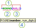
1. Structure. The structure of a function begins with an equal sign (=), followed by the function name, an opening parenthesis, the arguments for the function separated by commas, and a closing parenthesis.
2. Function name. For a list of available functions, click a cell and press SHIFT+F3.
3. Arguments. Arguments can be numbers, text, logical values such as TRUE or FALSE, arrays, error values such as #N/A, or cell references. The argument you designate must produce a valid value for that argument. Arguments can also be constants, formulas, or other functions.
4. Argument tooltip. A tooltip with the syntax and arguments appears as you type the function. For example, type =ROUND( and the tooltip appears. Tooltips appear only for built-in functions.
Entering functions
When you create a formula that contains a function, you can use the Insert Function dialog box to help you enter worksheet functions. As you enter a function into the formula, the Insert Function dialog box displays the name of the function, each of its arguments, a description of the function and each argument, the current result of the function, and the current result of the entire formula.
To make it easier to create and edit formulas and minimize typing and syntax errors, use Formula AutoComplete. After you type an = (equal sign) and beginning letters or a display trigger, Excel for the web displays, below the cell, a dynamic drop-down list of valid functions, arguments, and names that match the letters or trigger. You can then insert an item from the drop-down list into the formula.
Nesting functions
In certain cases, you may need to use a function as one of the arguments of another function. For example, the following formula uses a nested AVERAGE function and compares the result with the value 50.
1. The AVERAGE and SUM functions are nested within the IF function.
Valid returns When a nested function is used as an argument, the nested function must return the same type of value that the argument uses. For example, if the argument returns a TRUE or FALSE value, the nested function must return a TRUE or FALSE value. If the function doesn’t, Excel for the web displays a #VALUE! error value.
Nesting level limits A formula can contain up to seven levels of nested functions. When one function (we’ll call this Function B) is used as an argument in another function (we’ll call this Function A), Function B acts as a second-level function. For example, the AVERAGE function and the SUM function are both second-level functions if they are used as arguments of the IF function. A function nested within the nested AVERAGE function is then a third-level function, and so on.
Using references in formulas
A reference identifies a cell or a range of cells on a worksheet, and tells Excel for the web where to look for the values or data you want to use in a formula. You can use references to use data contained in different parts of a worksheet in one formula or use the value from one cell in several formulas. You can also refer to cells on other sheets in the same workbook, and to other workbooks. References to cells in other workbooks are called links or external references.
The A1 reference style
The default reference style By default, Excel for the web uses the A1 reference style, which refers to columns with letters (A through XFD, for a total of 16,384 columns) and refers to rows with numbers (1 through 1,048,576). These letters and numbers are called row and column headings. To refer to a cell, enter the column letter followed by the row number. For example, B2 refers to the cell at the intersection of column B and row 2.
|
To refer to |
Use |
|
The cell in column A and row 10 |
A10 |
|
The range of cells in column A and rows 10 through 20 |
A10:A20 |
|
The range of cells in row 15 and columns B through E |
B15:E15 |
|
All cells in row 5 |
5:5 |
|
All cells in rows 5 through 10 |
5:10 |
|
All cells in column H |
H:H |
|
All cells in columns H through J |
H:J |
|
The range of cells in columns A through E and rows 10 through 20 |
A10:E20 |
Making a reference to another worksheet In the following example, the AVERAGE worksheet function calculates the average value for the range B1:B10 on the worksheet named Marketing in the same workbook.
1. Refers to the worksheet named Marketing
2. Refers to the range of cells between B1 and B10, inclusively
3. Separates the worksheet reference from the cell range reference
The difference between absolute, relative and mixed references
Relative references A relative cell reference in a formula, such as A1, is based on the relative position of the cell that contains the formula and the cell the reference refers to. If the position of the cell that contains the formula changes, the reference is changed. If you copy or fill the formula across rows or down columns, the reference automatically adjusts. By default, new formulas use relative references. For example, if you copy or fill a relative reference in cell B2 to cell B3, it automatically adjusts from =A1 to =A2.
Absolute references An absolute cell reference in a formula, such as $A$1, always refer to a cell in a specific location. If the position of the cell that contains the formula changes, the absolute reference remains the same. If you copy or fill the formula across rows or down columns, the absolute reference does not adjust. By default, new formulas use relative references, so you may need to switch them to absolute references. For example, if you copy or fill an absolute reference in cell B2 to cell B3, it stays the same in both cells: =$A$1.
Mixed references A mixed reference has either an absolute column and relative row, or absolute row and relative column. An absolute column reference takes the form $A1, $B1, and so on. An absolute row reference takes the form A$1, B$1, and so on. If the position of the cell that contains the formula changes, the relative reference is changed, and the absolute reference does not change. If you copy or fill the formula across rows or down columns, the relative reference automatically adjusts, and the absolute reference does not adjust. For example, if you copy or fill a mixed reference from cell A2 to B3, it adjusts from =A$1 to =B$1.
The 3-D reference style
Conveniently referencing multiple worksheets If you want to analyze data in the same cell or range of cells on multiple worksheets within a workbook, use a 3-D reference. A 3-D reference includes the cell or range reference, preceded by a range of worksheet names. Excel for the web uses any worksheets stored between the starting and ending names of the reference. For example, =SUM(Sheet2:Sheet13!B5) adds all the values contained in cell B5 on all the worksheets between and including Sheet 2 and Sheet 13.
-
You can use 3-D references to refer to cells on other sheets, to define names, and to create formulas by using the following functions: SUM, AVERAGE, AVERAGEA, COUNT, COUNTA, MAX, MAXA, MIN, MINA, PRODUCT, STDEV.P, STDEV.S, STDEVA, STDEVPA, VAR.P, VAR.S, VARA, and VARPA.
-
3-D references cannot be used in array formulas.
-
3-D references cannot be used with the intersection operator (a single space) or in formulas that use implicit intersection.
What occurs when you move, copy, insert, or delete worksheets The following examples explain what happens when you move, copy, insert, or delete worksheets that are included in a 3-D reference. The examples use the formula =SUM(Sheet2:Sheet6!A2:A5) to add cells A2 through A5 on worksheets 2 through 6.
-
Insert or copy If you insert or copy sheets between Sheet2 and Sheet6 (the endpoints in this example), Excel for the web includes all values in cells A2 through A5 from the added sheets in the calculations.
-
Delete If you delete sheets between Sheet2 and Sheet6, Excel for the web removes their values from the calculation.
-
Move If you move sheets from between Sheet2 and Sheet6 to a location outside the referenced sheet range, Excel for the web removes their values from the calculation.
-
Move an endpoint If you move Sheet2 or Sheet6 to another location in the same workbook, Excel for the web adjusts the calculation to accommodate the new range of sheets between them.
-
Delete an endpoint If you delete Sheet2 or Sheet6, Excel for the web adjusts the calculation to accommodate the range of sheets between them.
The R1C1 reference style
You can also use a reference style where both the rows and the columns on the worksheet are numbered. The R1C1 reference style is useful for computing row and column positions in macros. In the R1C1 style, Excel for the web indicates the location of a cell with an «R» followed by a row number and a «C» followed by a column number.
|
Reference |
Meaning |
|
R[-2]C |
A relative reference to the cell two rows up and in the same column |
|
R[2]C[2] |
A relative reference to the cell two rows down and two columns to the right |
|
R2C2 |
An absolute reference to the cell in the second row and in the second column |
|
R[-1] |
A relative reference to the entire row above the active cell |
|
R |
An absolute reference to the current row |
When you record a macro, Excel for the web records some commands by using the R1C1 reference style. For example, if you record a command, such as clicking the AutoSum button to insert a formula that adds a range of cells, Excel for the web records the formula by using R1C1 style, not A1 style, references.
Using names in formulas
You can create defined names to represent cells, ranges of cells, formulas, constants, or Excel for the web tables. A name is a meaningful shorthand that makes it easier to understand the purpose of a cell reference, constant, formula, or table, each of which may be difficult to comprehend at first glance. The following information shows common examples of names and how using them in formulas can improve clarity and make formulas easier to understand.
|
Example Type |
Example, using ranges instead of names |
Example, using names |
|
Reference |
=SUM(A16:A20) |
=SUM(Sales) |
|
Constant |
=PRODUCT(A12,9.5%) |
=PRODUCT(Price,KCTaxRate) |
|
Formula |
=TEXT(VLOOKUP(MAX(A16,A20),A16:B20,2,FALSE),»m/dd/yyyy») |
=TEXT(VLOOKUP(MAX(Sales),SalesInfo,2,FALSE),»m/dd/yyyy») |
|
Table |
A22:B25 |
=PRODUCT(Price,Table1[@Tax Rate]) |
Types of names
There are several types of names that you can create and use.
Defined name A name that represents a cell, range of cells, formula, or constant value. You can create your own defined name. Also, Excel for the web sometimes creates a defined name for you, such as when you set a print area.
Table name A name for an Excel for the web table, which is a collection of data about a particular subject that is stored in records (rows) and fields (columns). Excel for the web creates a default Excel for the web table name of «Table1», «Table2», and so on, each time you insert an Excel for the web table, but you can change these names to make them more meaningful.
Creating and entering names
You create a name by using Create a name from selection. You can conveniently create names from existing row and column labels by using a selection of cells in the worksheet.
Note: By default, names use absolute cell references.
You can enter a name by:
-
Typing Typing the name, for example, as an argument to a formula.
-
Using Formula AutoComplete Use the Formula AutoComplete drop-down list, where valid names are automatically listed for you.
Using array formulas and array constants
Excel for the web doesn’t support creating array formulas. You can view the results of array formulas created in Excel desktop application, but you can’t edit or recalculate them. If you have the Excel desktop application, click Open in Excel to work with arrays.
The following array example calculates the total value of an array of stock prices and shares, without using a row of cells to calculate and display the individual values for each stock.
When you enter the formula ={SUM(B2:D2*B3:D3)} as an array formula, it multiples the Shares and Price for each stock, and then adds the results of those calculations together.
To calculate multiple results Some worksheet functions return arrays of values, or require an array of values as an argument. To calculate multiple results with an array formula, you must enter the array into a range of cells that has the same number of rows and columns as the array arguments.
For example, given a series of three sales figures (in column B) for a series of three months (in column A), the TREND function determines the straight-line values for the sales figures. To display all the results of the formula, it is entered into three cells in column C (C1:C3).
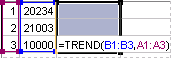
When you enter the formula =TREND(B1:B3,A1:A3) as an array formula, it produces three separate results (22196, 17079, and 11962), based on the three sales figures and the three months.
Using array constants
In an ordinary formula, you can enter a reference to a cell containing a value, or the value itself, also called a constant. Similarly, in an array formula you can enter a reference to an array, or enter the array of values contained within the cells, also called an array constant. Array formulas accept constants in the same way that non-array formulas do, but you must enter the array constants in a certain format.
Array constants can contain numbers, text, logical values such as TRUE or FALSE, or error values such as #N/A. Different types of values can be in the same array constant — for example, {1,3,4;TRUE,FALSE,TRUE}. Numbers in array constants can be in integer, decimal, or scientific format. Text must be enclosed in double quotation marks — for example, «Tuesday».
Array constants cannot contain cell references, columns or rows of unequal length, formulas, or the special characters $ (dollar sign), parentheses, or % (percent sign).
When you format array constants, make sure you:
-
Enclose them in braces ( { } ).
-
Separate values in different columns by using commas (,). For example, to represent the values 10, 20, 30, and 40, you enter {10,20,30,40}. This array constant is known as a 1-by-4 array and is equivalent to a 1-row-by-4-column reference.
-
Separate values in different rows by using semicolons (;). For example, to represent the values 10, 20, 30, and 40 in one row and 50, 60, 70, and 80 in the row immediately below, you enter a 2-by-4 array constant: {10,20,30,40;50,60,70,80}.