
Excel for Microsoft 365 Excel for Microsoft 365 for Mac Excel for the web Excel 2021 Excel 2021 for Mac Excel 2019 Excel 2019 for Mac Excel 2016 Excel 2016 for Mac Excel 2013 Excel 2010 Excel 2007 Excel for Mac 2011 Excel Starter 2010 More…Less
This article describes the formula syntax and usage of the SUBTOTAL function in Microsoft Excel.
Description
Returns a subtotal in a list or database. It is generally easier to create a list with subtotals by using the Subtotal command in the Outline group on the Data tab in the Excel desktop application. Once the subtotal list is created, you can modify it by editing the SUBTOTAL function.
Syntax
SUBTOTAL(function_num,ref1,[ref2],…)
The SUBTOTAL function syntax has the following arguments:
-
Function_num Required. The number 1-11 or 101-111 that specifies the function to use for the subtotal. 1-11 includes manually-hidden rows, while 101-111 excludes them; filtered-out cells are always excluded.
|
Function_num |
Function_num |
Function |
|---|---|---|
|
1 |
101 |
AVERAGE |
|
2 |
102 |
COUNT |
|
3 |
103 |
COUNTA |
|
4 |
104 |
MAX |
|
5 |
105 |
MIN |
|
6 |
106 |
PRODUCT |
|
7 |
107 |
STDEV |
|
8 |
108 |
STDEVP |
|
9 |
109 |
SUM |
|
10 |
110 |
VAR |
|
11 |
111 |
VARP |
-
Ref1 Required. The first named range or reference for which you want the subtotal.
-
Ref2,… Optional. Named ranges or references 2 to 254 for which you want the subtotal.
Remarks
-
If there are other subtotals within ref1, ref2,… (or nested subtotals), these nested subtotals are ignored to avoid double counting.
-
For the function_num constants from 1 to 11, the SUBTOTAL function includes the values of rows hidden by the Hide Rows command under the Hide & Unhide submenu of the Format command in the Cells group on the Home tab in the Excel desktop application. Use these constants when you want to subtotal hidden and nonhidden numbers in a list. For the function_Num constants from 101 to 111, the SUBTOTAL function ignores values of rows hidden by the Hide Rows command. Use these constants when you want to subtotal only nonhidden numbers in a list.
-
The SUBTOTAL function ignores any rows that are not included in the result of a filter, no matter which function_num value you use.
-
The SUBTOTAL function is designed for columns of data, or vertical ranges. It is not designed for rows of data, or horizontal ranges. For example, when you subtotal a horizontal range using a function_num of 101 or greater, such as SUBTOTAL(109,B2:G2), hiding a column does not affect the subtotal. But, hiding a row in a subtotal of a vertical range does affect the subtotal.
-
If any of the references are 3-D references, SUBTOTAL returns the #VALUE! error value.
Example
Copy the example data in the following table, and paste it in cell A1 of a new Excel worksheet. For formulas to show results, select them, press F2, and then press Enter. If you need to, you can adjust the column widths to see all the data.
|
Data |
||
|---|---|---|
|
120 |
||
|
10 |
||
|
150 |
||
|
23 |
||
|
Formula |
Description |
Result |
|
=SUBTOTAL(9,A2:A5) |
The sum of the subtotal of the cells A2:A5, using 9 as the first argument. |
303 |
|
=SUBTOTAL(1,A2:A5) |
The average of the subtotal of the cells A2:A5, using 1 as the first argument. |
75.75 |
|
Notes |
||
|
The SUBTOTAL function always requires a numeric argument (1 through 11, 101 through 111) as its first argument. This numeric argument is applied to the subtotal of the values (cell ranges, named ranges) that are specified as the arguments that follow. |
Need more help?
Purpose
Get a subtotal in a list or database
Return value
A number representing a specific kind of subtotal
Usage notes
The SUBTOTAL function is designed to run a given calculation on a range of cells while ignoring cells that should not be included. SUBTOTAL has three features that make it especially useful:
- It automatically ignores cells that have been filtered out of view.
- It automatically ignores existing subtotal formulas to avoid double counting.
- It can perform many calculations, including SUM, AVERAGE, COUNT, MAX, MIN, and others.
Because SUBTOTAL ignores cells that have been «filtered out», it is especially useful in Excel Tables or filtered data. In addition, SUBTOTAL can be optionally set to exclude values in rows that have been manually hidden (i.e. rows hidden with a shortcut or by Right click > Hide). Regardless of the calculation performed, SUBTOTAL returns single aggregate result from a set of data. Finally, while SUBTOTAL is good at ignoring things, it does not ignore errors. If you need capability, see the AGGREGATE function.
Note: the SUBTOTAL function automatically ignores other SUBTOTAL formulas that exist in references to prevent double-counting.
Examples
Below are examples of SUBTOTAL configured to SUM, COUNT, and AVERAGE the values in a range. Notice the only difference is the value used for the function_num argument:
=SUBTOTAL(109,range) // SUM
=SUBTOTAL(103,range) // COUNT
=SUBTOTAL(101,range) // AVERAGE
In the worksheet shown above, the formulas in C4 and F4 are:
=SUBTOTAL(3,B7:B19) // count visible
=SUBTOTAL(9,F7:F19) // sum visible
Available calculations
The calculation performed by SUBTOTAL is determined by the function_num argument, which is given as a number. There are 11 calculations total, each with two options, as seen below. Notice these values are «paired» (e.g. 1-101, 2-102, 3-103, and so on). This is related to how SUBTOTAL deals with manually hidden rows. When function_num is between 1-11, SUBTOTAL includes rows that have been manually hidden. When function_num is between 101-111, SUBTOTAL excludes rows that have been manually hidden.
| Function | Include hidden | Ignore hidden |
| AVERAGE | 1 | 101 |
| COUNT | 2 | 102 |
| COUNTA | 3 | 103 |
| MAX | 4 | 104 |
| MIN | 5 | 105 |
| PRODUCT | 6 | 106 |
| STDEV | 7 | 107 |
| STDEVP | 8 | 108 |
| SUM | 9 | 109 |
| VAR | 10 | 110 |
| VARP | 11 | 111 |
Note: SUBTOTAL always ignores values in cells that are hidden with a filter. Values in rows that have been «filtered out» are never included, regardless of function_num.
SUBTOTAL in Excel Tables
The SUBTOTAL function is used when you display a Total row in an Excel Table. Excel inserts the SUBTOTAL function automatically, and you can use a drop-down menu to switch behavior and show max, min, average, etc. Excel uses SUBTOTAL for calculations in the Total row of an Excel Table because SUBTOTAL automatically excludes rows hidden by the filter controls at the top of the table. That is, as you filter rows in a table with a Total row, calculations automatically respect the filter.
SUBTOTAL with outlines
Excel has a Subtotal feature that automatically inserts SUBTOTAL formulas in sorted data. You can find this feature at Data > Outline > Subtotal. SUBTOTAL formulas inserted this way use the standard function numbers 1-11. This allows the subtotal results to remain visible even as rows are hidden and displayed when the outline is collapsed and expanded.
Note: although the Outline feature is an «easy» way to insert subtotals in a set of data, a Pivot Table is a better and more flexible way to analyze data. In addition, a Pivot Table will separate the data from the presentation of the data, which is a best practice.
Notes
- When function_num is between 1-11, SUBTOTAL includes manually hidden rows.
- When function_num is between 101-111, SUBTOTAL excludes manually hidden rows.
- In filtered lists, SUBTOTAL always ignores values in hidden rows, regardless of function_num.
- SUBTOTAL ignores other SUBTOTAL formulas that exist in references to prevent double-counting.
- SUBTOTAL works with vertical data. In horizontal ranges, values in hidden columns are always included.
The SUBTOTAL excel function performs different arithmetic operations like average, product, sum, standard deviation, variance etc., on a defined range. Each operation has a unique function number assigned to it. This function number is supplied as an argument to the SUBTOTAL function.
For example, a worksheet consists of the following values in column A:
- Cell A1 contains 22
- Cell A2 contains 45
- Cell A3 contains 37
- Cell A4 contains 12
The formula “=SUBTOTAL(1,A1:A4)” returns 29. This output is the average of the given range (A1:A4). The number 1 in the formula tells Excel that the average of the listed numbers is to be calculated.
With the SUBTOTAL function, one can either include or exclude the values of the hidden rows. However, the filtered-out values (the values hidden by a filter) are excluded, by default.
The SUBTOTAL function works with vertical ranges (columns) of a dataset. It can perform 11 different arithmetic operations on a dataset. The SUBTOTAL function is categorized under the Math and Trigonometry functions of Excel.
The SUBTOTAL is a versatile function which is available in all versions of Excel. In the modern versions of Excel, the AGGREGATE functionAGGREGATE Function in excel returns the aggregate of a given data table or data lists.read more is also available. This can perform more operations compared to the SUBTOTAL excel function.
Table of contents
- What is SUBTOTAL Function in Excel?
- Syntax of the SUBTOTAL in Excel
- Operations Performed by the SUBTOTAL Function
- How to Open the SUBTOTAL Function in Excel?
- How to use the SUBTOTAL Function in Excel?
- Example #1
- Example #2
- Example #3
- Example #4
- Example #5
- Example #6
- Example #7
- Example #8
- Example #9
- Example #10
- Example #11
- Properties
- Errors Returned by the SUBTOTAL Function
- Frequently Asked Questions
- SUBTOTAL Excel Function Video
- Recommended Articles
Syntax of the SUBTOTAL in Excel
The syntax of the SUBTOTAL function of Excel is shown in the following image:
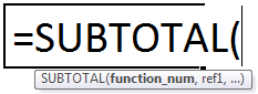
The SUBTOTAL function accepts the following arguments:
- Function_num: This is the number that determines which arithmetic operation (function) will be performed by the SUBTOTAL function. The “function_num” argument can take any value from 1 to 11 or 101 to 111.
- Ref1: This is the range of cells on which the arithmetic operation is to be performed. It can be supplied as a reference or as a named range.
- Ref2: This is the second range of cells on which the arithmetic operation is to be performed. This also can be entered as a reference or as a named range.
The arguments “function_num” and “ref1” are mandatory, while “ref2” is optional. The SUBTOTAL function returns a numeric output.
Note: The “function_num” argument is always entered as a numeric value.
Operations Performed by the SUBTOTAL Function
The SUBTOTAL function performs an arithmetic operation depending on the value of the “function_num” argument. The operations (functions) performed by the SUBTOTAL function and the corresponding function numbers are listed as follows:
| Function | function_num Includes hidden values |
function_num Excludes hidden values |
|---|---|---|
| AVERAGE | 1 | 101 |
| COUNT | 2 | 102 |
| COUNTA | 3 | 103 |
| MAX | 4 | 104 |
| MIN | 5 | 105 |
| PRODUCT | 6 | 106 |
| STDEV | 7 | 107 |
| STDEVP | 8 | 108 |
| SUM | 9 | 109 |
| VAR | 10 | 110 |
| VARP | 11 | 111 |
One must observe that for every operation (function), there are two values (like 1 and 101 for AVERAGE) of the “function_num” argument. The “function_num” argument can take either of these values depending on whether the hidden rows are included or excluded from the subtotals.
The values of the “function_num” argument have the following implications:
- When the value of “function_num” is between 1-11, the SUBTOTAL includes the manually hidden rows in the calculations.
- When the value of “function_num” is between 101-111, the SUBTOTAL excludes the manually hidden rows from the calculations.
The values of rows hidden by a filter are always excluded irrespective of the “function_num” argument.
Note: The user need not memorize the function numbers. This is because as soon as one begins to type the SUBTOTAL formula in a cell, Excel displays a list containing the different operations and the corresponding function numbers. To select the operation to be performed, double-click its name displayed in the list.
How to Open the SUBTOTAL Function in Excel?
You can download this SUBTOTAL Function Excel Template here – SUBTOTAL Function Excel Template
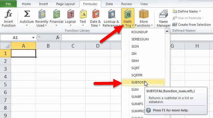
To open the SUBTOTAL excel function, enter “=SUBTOTAL” in the required cell, followed by the arguments of the function. Alternatively, the SUBTOTAL function can be opened from the Formulas tab of Excel. The steps for the same are listed as follows:
- Select the cell in which the SUBTOTAL formula is to be entered.
- From the Formulas tab, click the drop-down of “Math & Trig”. Select “SUBTOTAL”, as shown in the following image.

- The “function arguments” dialog box opens, as shown in the following image. Enter the values for the arguments “function_num” and “ref1”. Once the cursor is placed inside the “ref1” box, the “ref2” box appears below it.
Click “Ok” to proceed. The output of the SUBTOTAL function will be displayed in the cell selected in step 1.


How to use the SUBTOTAL Function in Excel?
Let us consider some examples to understand the working of the SUBTOTAL function of Excel.
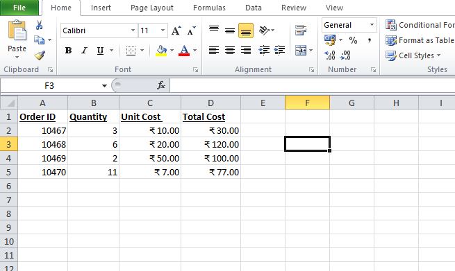
The succeeding image shows the IDs of four orders (in column A) received by an organization. Prior to completing these orders, the organization has compiled a dataset which contains the following information:
- The quantities of goods to be supplied are listed in column B.
- The unit costs of each good are given in column C.
- The total costs of each order are shown in column D.
There are no hidden rows and filters in the given dataset. Perform the following tasks:
- Apply all the 11 operations of the SUBTOTAL excel function to the range D2:D5. Cover one operation in one example. So, there must be 11 examples subsequent to the succeeding image.
- At the end of example #11, the formulas and the results of all the examples must be consolidated at one place.
Let us begin with the different operations of the SUBTOTAL excel function covered in the following examples.
Note: Please ignore the small boxes containing question marks (in columns C and D) in the images of all the eleven examples.
Example #1
Let us apply the AVERAGE functionThe AVERAGE function in Excel gives the arithmetic mean of the supplied set of numeric values. This formula is categorized as a Statistical Function. The average formula is =AVERAGE(read more with the SUBTOTAL formula. This helps calculate the average of the defined range. The steps for the same are listed as follows:
Step 1: Enter the following formula in cell F2.
“=SUBTOTAL(1,D2:D5)”
Note: To select the function number 1, double-click “1-AVERAGE” appearing in the list of the available arithmetic operations. Alternatively, one can type “1” (without the double quotation marks) manually.
Step 2: Press the “Enter” key. The output is 81.75, which appears in cell F2. The same is shown in the following image.
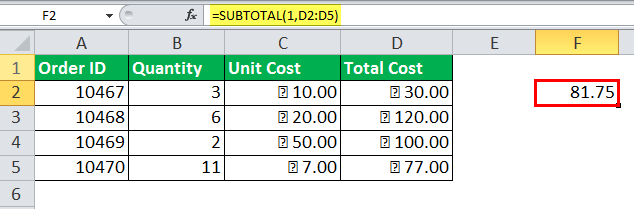
Explanation: The first argument of the given SUBTOTAL excel formula (entered in step 1) is 1, which implies that the average needs to be calculated. The second argument is the range D2:D5. So, the average is computed for the range D2:D5. Hence, the output of the formula is 81.75.
Since there are no hidden rows, we have used 1 as the function number. Had there been a hidden row, we would have applied the formula “=SUBTOTAL(101,D2:D5).” This formula would have excluded the hidden row and performed the given operation (average) on the visible rows of the range D2:D5.
For instance, if rows 3 and 5 had been hidden, the formula “=SUBTOTAL(101,D2:D5)” would have returned 65. This is the average of the numbers 30 and 100.
Example #2
Let us apply the COUNT functionThe COUNT function in excel counts the number of cells containing numerical values within the given range. It is a statistical function and returns an integer value. The syntax of the COUNT formula is “=COUNT(value 1, [value 2],…)”
read more with the SUBTOTAL excel formula. This helps count the numeric values of the defined range. The steps are listed as follows:
Step 1: Enter the following formula in cell F2.
“=SUBTOTAL(2,D2:D5)”
Note: Double-click “2-COUNT” from the list of operations. In this way, the function number 2 appears in the SUBTOTAL formula.
Step 2: Press the “Enter” key. The output 4 appears in cell F2, as shown in the following image.
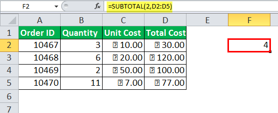
Explanation: The “function_num” is 2 and “ref1” is D2:D5. So, the COUNT function is applied to the range D2:D5. The COUNT function counts the number of cells containing numeric values in the range D2:D5.
There are four numeric cells in the range D2:D5. These cells are D2, D3, D4, and D5. Hence, the output of the SUBTOTAL function is 4.
Note: The COUNT function counts those cells of a range which contain numbers (positive and negative both), dates, times, decimal numbers, percentages, and so on. It does not count the empty cells, error values, logical values (Boolean values true and false), and text strings.
Example #3
Let us apply the COUNTA functionThe COUNTA function is an inbuilt statistical excel function that counts the number of non-blank cells (not empty) in a cell range or the cell reference. For example, cells A1 and A3 contain values but, cell A2 is empty. The formula “=COUNTA(A1,A2,A3)” returns 2.
read more with the SUBTOTAL excel formula. This helps count the non-blank cells of the defined range. The steps for the same are listed as follows:
Step 1: Enter the following formula in cell F2.
“=SUBTOTAL(3,D2:D5)”
Note: To enter 3 as the “function_num” in the SUBTOTAL formula, double-click “3-COUNTA” from the list displayed in Excel.
Step 2: Press the “Enter” key. The output is 4 in cell F2, as shown in the following image.
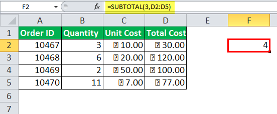
Explanation: The “function_num” argument is 3 and the “ref1” argument is D2:D5. The given SUBTOTAL formula (entered in step 1) counts the non-empty cells in the range D2:D5.
The non-empty cells in the given range (D2:D5) are D2, D3, D4, and D5. Hence, the output of the SUBTOTAL formula is 4.
Note: The COUNTA function counts the cells containing text strings, numbers, logical (Boolean) values, date/time values, error values, and so on. Only the absolutely empty cells are excluded from the count.
Example #4
Let us apply the MAX functionThe MAX Formula in Excel is used to calculate the maximum value from a set of data/array. It counts numbers but ignores empty cells, text, the logical values TRUE and FALSE, and text values.read more with the SUBTOTAL excel formula. This helps find the largest value of the defined range. The steps for the same are listed as follows:
Step 1: Enter the following formula in cell F2.
“=SUBTOTAL(4,D2:D5)”
Note: To select the “function_num” 4, double-click “4-MAX” from the list displayed in Excel. Alternatively, one can type “4” (without the double quotation marks) manually.
Step 2: Press the “Enter” key. The output in cell F2 is 120. It is shown in the following image.
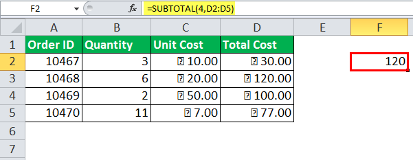
Explanation: The MAX function returns the largest numeric value from a series of numbers. With the given SUBTOTAL formula (entered in step 1), the largest value of the range D2:D5 is 120. Hence, the output is 120.
Had we hidden the rows 3 and 4, the formula “=SUBTOTAL(104,D2:D5)” would have returned 77. This is because 77 is the larger of the two visible values (30 and 77). So, the function number 104 excludes the values of the hidden rows while finding the maximum number of a range.
Note: The MAX function considers the numerical values of a dataset. If a range consists of text strings, logical values (true and false) or empty strings, they are ignored by the MAX function.
Example #5
Let us apply the MIN function with the SUBTOTAL excel formula. This helps find the smallest value of the defined range. The steps are listed as follows:
Step 1: Enter the following formula in cell F2.
“=SUBTOTAL(5,D2:D5)”
Note: Double-click “5-MIN” (in the list of functions) to enter 5 as the “function_num” argument.
Step 2: Press the “Enter” key. The output in cell F2 is 30, as shown in the following image.
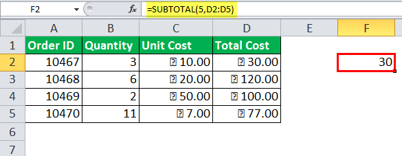
Explanation: The MIN function returns the smallest value from a list of numbers. Here, the smallest number of the range D2:D5 is 30.
Hence, the output of the SUBTOTAL formula (entered in step 1) is 30.
Note: Like the MAX function, the MIN also works with numerical values of a range. The MIN function ignores the text strings, empty strings, and logical values.
Example #6
Let us apply the PRODUCT functionProduct excel function is an inbuilt mathematical function which is used to calculate the product or multiplication of the given numbers. If you provide this formula arguments as 2 and 3 as =PRODUCT(2,3) then the result displayed is 6.read more with the SUBTOTAL excel formula. This helps perform the multiplication of the defined range of numbers. The steps for the same are listed as follows:
Step 1: Enter the following formula in cell F2.
“=SUBTOTAL(6,D2:D5)”
Note: To enter 6 as the “function_num” argument, double-click “6-PRODUCT” from the list of functions.
Step 2: Press the “Enter” key. The output is 27720000. Since this number is quite big, we have retained its scientific notation in cell F2. For this, perform the following tasks:
- Select cell F2 and right-click it.
- Select “format cells” from the context menu.
- Under “category,” select “scientific.” In “decimal places,” enter “1.”
- Click “Ok.”
The scientific notation 2.8E+07 appears in cell F2, as shown in the following image. The SUBTOTAL formula can also be seen in the formula bar. The output 27720000 can be viewed in the image at the end of example #11, which shows the consolidated results.
Note 1: The scientific notation displays a number in the exponential format. In Excel, scientific notations are often used to shorten large numeric values. By using a scientific notation, the appearance of a cell value changes. However, the value itself does not change.
Note 2: The preview of the formatted number can be seen under “sample” in the “format cells” dialog box.
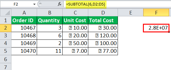
Explanation: The SUBTOTAL formula (entered in step 1) performs the multiplication operation on the range D2:D5. This works as follows:
30*120*100*77=27720000
Hence, the output (27720000) is the product of the numbers in cells D2, D3, D4, and D5.
Had we hidden the rows 3 and 4, the formula “=SUBTOTAL(106,D2:D5)” would have returned 2310. This is the product of the visible cells D2 and D5.
Example #7
Let us apply the STDEV or STDEV.S functionThe standard deviation shows the variability of the data values from the mean (average). In Excel, the STDEV and STDEV.S calculate sample standard deviation while STDEVP and STDEV.P calculate population standard deviation. STDEV is available in Excel 2007 and the previous versions. However, STDEV.P and STDEV.S are only available in Excel 2010 and subsequent versions.
read more with the SUBTOTAL excel formula. This helps calculate the standard deviation of a population based on a data sample. The steps for the same are listed as follows:
Step 1: Enter the following formula in cell F2.
“=SUBTOTAL(7,D2:D5)”
Note: Double-click “7-STDEV” or “7-STDEV.S” to select the function number 7.
Step 2: Press the “Enter” key. The output is 38.7158, as shown in the following image.
Note: Population refers to the entire dataset, while a sample is a subset of this dataset. In other words, a sample contains one or more elements of the population.

Explanation: The STDEV and STDEV.S calculate the standard deviation by assuming the range D2:D5 as a sample of the population. Hence, the sample standard deviation is 38.7158. This is the output of the SUBTOTAL formula entered in step 1.
While calculating the sample standard deviation, “n-1” is taken as the denominator, where “n” is the number of values in a dataset.
The high standard deviation (38.7158) implies that the values of the given range (D2:D5) fluctuate from the mean (average) to a great extent.
Note 1: The standard deviation indicates the dispersionIn statistics, dispersion (or spread) is a means of describing the extent of distribution of data around a central value or point. It aids in understanding data distribution.read more (deviation) of the data values from the mean (average). In other words, with standard deviation, one can say whether the data values are close or spread out from the mean.
Note 2: Both STDEV and STDEV.S are sample standard deviations that help make relevant conclusions for the population. The STDEV.S is an improved version of the STDEV function. STDEV.S is available in Excel 2010 and the subsequent versions.
Note 3: Both STDEV and STDEV.S ignore the text strings and the logical values of the data sample.
Example #8
Let us apply the STDEVP or STDEV.P function with the SUBTOTAL excel formula. This helps calculate the standard deviation of the entire population. The steps are listed as follows:
Step 1: In cell F2, enter the following formula.
“=SUBTOTAL(8,D2:D5)”
Note: Double-click “8-STDEVP” or “8-STDEV.P” to enter function number 8. Alternatively, one can type “8” (without the double quotation marks) manually.
Step 2: Press the “Enter” key. The output in cell F2 is 33.5289. The same is shown in the following image.

Explanation: The STDEVP and STDEV.P functions assume that the data supplied as an argument (range D2:D5) represents the entire population. Hence, the SUBTOTAL formula (entered in step 1) returns the population standard deviation, which is 33.5289.
While calculating the population standard deviation, “n” is taken as the denominator, where “n” is the number of values in a dataset.
The high standard deviation (33.5289) indicates high variability of the supplied values (range D2:D5) from the mean (average).
Note: Both the STDEVP and STDEV.P functions ignore the text strings and logical values of the population dataset. The STDEV.P is an improved version of STDEVP. The STDEV.P function is available in Excel 2010 and the newer versions.
Example #9
Let us apply the SUM functionThe SUM function in excel adds the numerical values in a range of cells. Being categorized under the Math and Trigonometry function, it is entered by typing “=SUM” followed by the values to be summed. The values supplied to the function can be numbers, cell references or ranges.read more with the SUBTOTAL excel formula. This helps to sum up the numeric values of the defined range. The steps are listed as follows:
Step 1: In cell F2, enter the following formula.
“=SUBTOTAL(9,D2:D5)”
Note: To enter function number 9, double-click “9-SUM” displayed in the Excel list of functions. Alternatively, type the number “9” (without the double quotation marks) manually.
Step 2: Press the “Enter” key. The output in cell F2 is 327. It is shown in the following image.

Explanation: The SUM function adds the values of the range D2:D5. It works as follows:
30+120+100+77=327
Hence, the output of the SUBTOTAL formula (entered in step 1) is 327.
Had we hidden the rows 3 and 4, the formula “=SUBTOTAL(109,D2:D5)” would have returned 107. This addition considers the values of the visible cells (D2 and D5) only.
Note: The SUM function ignores the empty cells and the text strings of the dataset.
Example #10
Let us apply the VAR or VAR.S function with the SUBTOTAL excel function. This calculates the variance of a population based on a data sample. The steps for the same are listed as follows:
Step 1: Enter the following formula in cell F2.
“=SUBTOTAL(10,D2:D5)”
Note: To enter 10 in the SUBTOTAL formula, double-click “10-VAR” or “10-VAR.S” from the list of functions.
Step 2: Press the “Enter” key. The output is 1498.92, as shown in the following image.

Explanation: The VAR and VAR.S functions assume that the values supplied (range D2:D5) as an argument are a sample of the population. Hence, the sample variance returned by the SUBTOTAL formula (entered in step 1) is 1498.92.
Since the output (1498.92) is large, it indicates high variance or high volatility (risk). When the variance is high, the following is inferred:
- The sample values (range D2:D5) supplied are far from the mean (average).
- The sample values are more spread out from each other.
Note 1: The sample variance is the square of the sample standard deviation. When the variance is zero (output of the SUBTOTAL formula is 0), there is no variability in the values of the dataset. This implies that all the values of the dataset are identical.
Note 2: The VAR and VAR.S ignore the text strings and the logical values of the data sample. The VAR.S is an improved version of the VAR function. The VAR.S is available in Excel 2010 and all the subsequent versions.
Example #11
Let us apply the VARP or VAR.P function with the SUBTOTAL excel formula. This helps calculate the variance of the entire population. The steps for the same are listed as follows:
Step 1: In cell F2, enter the following formula.
“=SUBTOTAL(11,D2:D5)”
Note: Double-click “11-VARP” or “11-VAR.P” to enter 11 in the SUBTOTAL formula. Alternatively, one can type “11” (without the double quotation marks) manually.
Step 2: Press the “Enter” key. The output appears in cell F2. It is 1124.19, as shown in the following image.

Explanation: The VARP and the VAR.P functions assume that the supplied values (range D2:D5) represent the entire population. Hence, the output of the SUBTOTAL formula (entered in step 1) is the population variance. This figure is 1124.19.
The output (1124.19) is large, which implies that the values of the entire population (range D2:D5) are scattered (spread out). A high variance is associated with high volatility (risk).
Note: The population variance is the square of the population standard deviation. The VAR.P is an improved version of VARP. The VAR.P is available in Excel 2010 and the subsequent versions. The VARP and VAR.P both ignore the text strings and the logical values of the population dataset.
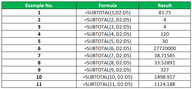
Let us consolidate the results of the preceding examples (example #1 to #11) in the succeeding image.
The formulas and the outputs are shown in the columns “formula” and “result” respectively. The example numbers (1-11) are shown in the first column titled “example no.”
Properties
The major features of the SUBTOTAL excel function are listed as follows:
Property 1: The SUBTOTAL function, with function number between 101-111, does not work with horizontal ranges. For instance, a worksheet contains the following data:
Cell A1 contains 2
Cell B1 contains 3
Cell C1 contains 4
Cell D1 contains 5
The formula “=SUBTOTAL(106,A1:D1)” returns 120. If column C is hidden, the formula “=SUBTOTAL(106,A1:D1)” returns 120 again. This implies that while performing an operation on a horizontal range, hiding a column does not impact the SUBTOTAL excel function.
However, hiding a row, while performing an operation on a vertical range, does impact the SUBTOTAL formula. This is true when the function number is between 101-111. In this case, the SUBTOTAL formula calculates an output by considering only the visible rows.
Hence, when the function number is between 101-111, the SUBTOTAL function works as follows:
- It includes the values of the hidden columns while working on a horizontal range.
- It excludes the values of the hidden rows while working on a vertical range.
Property 2: The SUBTOTAL excel function ignores the nested SUBTOTAL formulas while performing an arithmetic operation. This is done to prevent errors that may occur as a result of double counting.
Note 1: A nested function is one which is placed inside another function. The inner (nested) function is calculated first. The outcome of the inner function becomes an argument for the outer function.
Note 2: Double counting is an error whereby the same number is counted twice.
Errors Returned by the SUBTOTAL Function
The SUBTOTAL excel function returns the following errors:
- “#VALUE!” error: This error occurs due to either of the following reasons:
- If the function_num argument is not a permissible value (accepted values are integers between 1-11 or 101-111)
- If the range address supplied is a 3-D reference
- “#DIV/0!” error: This error occurs due to either of the following reasons:
- If a calculation involves division by zero
- If a function (arithmetic operation) works with only numbers, but the defined range does not contain any numeric value
- “#NAME?” error: This error occurs if the name of the SUBTOTAL function is spelt incorrectly.
Note: In a 3-D reference, the same range (or a cell) is referred on various worksheets. For instance, the reference Sheet1:Sheet3!A1:A5 is a 3-D reference of the range A1:A5. This reference involves the worksheets, “Sheet1,” “Sheet2, and “Sheet3.”
Frequently Asked Questions
1. Define the SUBTOTAL function of Excel.
The SUBTOTAL function performs a specified arithmetic operation (like average, minimum, maximum, count, product etc.) on a pre-defined range of cells. A total of 11 different operations can be performed by the SUBTOTAL function. Further, this function works with vertical ranges of a dataset.
The syntax of the SUBTOTAL function is stated as follows:
“SUBTOTAL(function_num,ref1,[ref2],…)”
The “function_num” is used to specify the operation (function) that will be performed by the SUBTOTAL function. The “ref1” and “ref2” are the first and the second range of cells respectively on which the operation is to be performed.
The “function_num” and “ref1” are mandatory arguments, while “ref2” is an optional argument. The function number 1-11 includes the rows hidden manually, while 101-111 excludes the values of hidden rows. The values of rows hidden by a filter are always excluded.
As a user begins to enter the SUBTOTAL formula in a cell, Excel displays a list of the available function numbers. One can double-click the required function number to select it.
2. Why is the SUBTOTAL function used in Excel?
The SUBTOTAL function is used for the following reasons:
a. It produces dynamic results in the case of filtered data. Once a filter is applied, the SUBTOTAL formula (with function number 101-111) automatically recalculates to include only the values visible after filtering. So, the output of the SUBTOTAL formula corresponds to the filters applied.
b. It ignores the values of the manually hidden rows. When one or more rows are hidden, the SUBTOTAL formula excludes such rows from the calculations. In this way, the arithmetic operations can be performed only on the relevant data.
c. It ignores the nested SUBTOTAL formulas. If a user has applied multiple SUBTOTAL formulas to the same range, only the outer subtotals are calculated. The inner (nested) subtotals are excluded from the calculations. In this way, several operations can be performed on the same range, without worrying about double counting.
d. It helps perform various arithmetic operations by using a single function. Had different functions been used for the different operations, the arguments of each function had to be remembered. So, the usage of the SUBTOTAL function eases working with Excel.
3. Where is the SUBTOTAL function in Excel?
In Excel, the SUBTOTAL function can be accessed in the following ways:
Method 1
a. Begin by typing “=SUBTOTAL” directly in a cell.
b. Type the function number and select the range on which the operation is to be performed.
c. Press the “Enter” key.
Method 2
a. Select a cell in which the subtotals are to be calculated.
b. Click the drop-down arrow of Math and Trigonometry from the Formulas tab. Select “subtotal”.
c. The “function arguments” dialog box appears. In this, enter the desired function number and the range on which the operation is to be performed.
d. Click “Ok” to apply the SUBTOTAL function.
Method 3
a. Select the dataset on which the SUBTOTAL function is to be applied.
b. From the Data tab, click “subtotal”. The “subtotal” dialog box appears.
c. In the box below “at each change in”, select the column whose entries are to be consolidated or grouped. The name of the operation will appear in this column after each group of rows.
d. In the box below “use function”, select the operation to be performed.
e. In the box below “add subtotal to”, select the column to which the SUBTOTAL formula should be applied. This column should contain the values that are to be subtotaled.
f. Select or deselect the following checkboxes:
• “Summary below data” – Select this checkbox if a summary row is required immediately below the dataset. If the summary row should be right below the column headers, deselect this checkbox.
• “Replace current subtotals” – Deselect this checkbox to prevent overwriting the already existing subtotals. In case there are no existing subtotal formulas, one may or may not select this checkbox.
• “Page break between groups” – Select this checkbox if the page breaks at the end of each subtotal are required.
g. Click “Ok” to apply the SUBTOTAL function.
The “plus” (+) and “minus” (-) boxes are created to the left side of the worksheet. These boxes can be used to expand or collapse the rows of the dataset.
Note: For method 3 to work correctly, ensure that every column has a label or header in the first row of the dataset. It is not advised to have blank rows or columns in the range on which the subtotals are to be applied.
SUBTOTAL Excel Function Video
Recommended Articles
This has been a guide to the SUBTOTAL in Excel. Here we discuss the SUBTOTAL formula in Excel and how to use it, along with examples and a downloadable Excel template. You may also look at these useful functions in Excel–
- SIGN FunctionThe sign function in excel is a Math/Trig function that returns the sign (-1, 0 or +1) of the numerical argument supplied to it.read more
- Find Links in ExcelExternal Links in Excel are the references to a cell or range specified in another workbook & you can find them manually by looking into Defined Names, Objects, Formulas, Chart Titles, & Chart Data Series. read more
You can sum up the subtotals in the Excel table using the built-in formulas and the corresponding command in the «Structure» group on the «Data» tab.
The important condition of using tools – the values are organized in the form of a list or a database, the same records are in the same group. When you create the summary report, the subtotals are generated automatically.
Calculation of subtotals in Excel
To demonstrate the calculation of subtotals in Excel, let’s take the small example. We suppose that a user has a list with the sales of certain goods:
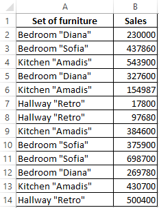
It is necessary to calculate the revenue from the sale of certain groups of goods. If you use a filter, you can get the same type of records according to the specified selection criteria. But the values will have to be calculated manually. Therefore, we will use another Microsoft Excel tool – the «Interim Results» command.
In order for the function to produce the correct result, check the range for the following conditions:
- The table is organized in the form of the simple list or database.
- The first line — shows the column names.
- The columns contain the same values.
- There are no empty rows or columns in the table.
Let’s start …
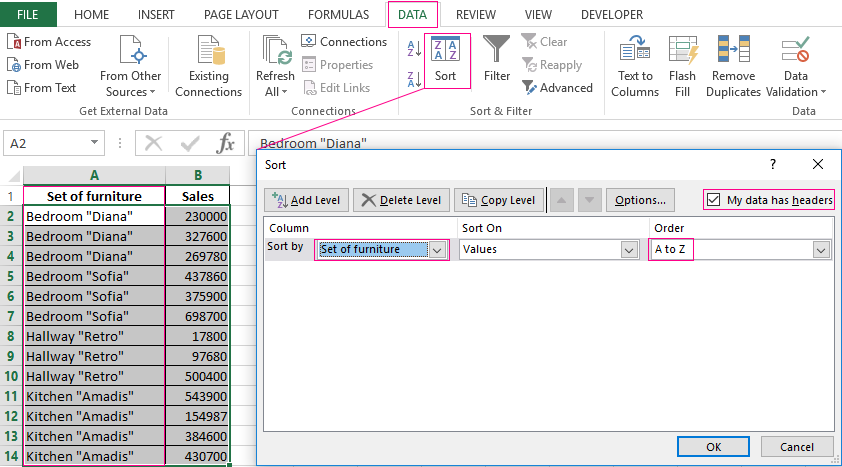
- We sort the range by the value of the first column — the same type of data should be near.
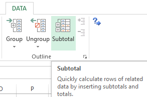
- Select any cell in the table. Select the «DATA» tab on the line. The group «Outline» – is the team «Subtotal».
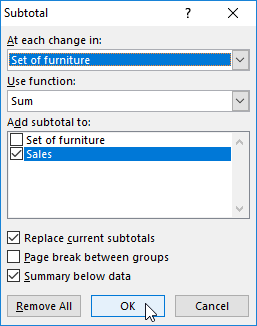
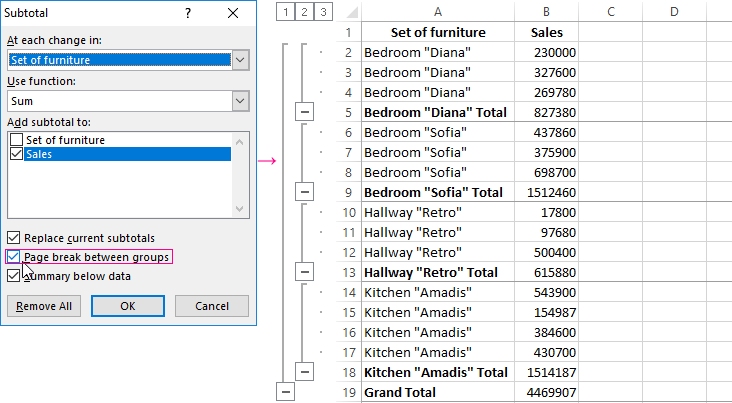
- We fill the dialog box in the «Subtotal». In the field «At each change in» we select the condition for data selection (in this example, «Value»). In the field «Use function:» we assign the function «Sum». In the «Add subtotal to» field, you should mark the columns to which the function will apply (Sales).
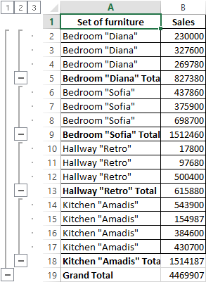
- Close the dialog box by clicking OK. The initial table acquires the following form:
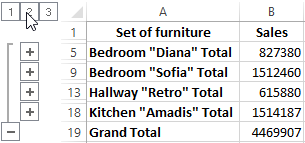
If you collapse the rows in the subgroups (click on the «minus» to the left of the line numbers), then we get the table only from the subtotals:
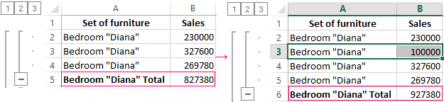
Each time the column «Set of furniture» is changed, the subtotal is recalculated in the «Sales» column.
In order for each intermediate result to be followed by a page break, in the dialog box you need to tick the «Page break between groups».
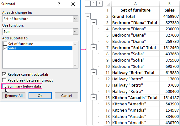
In order for intermediate data to be displayed OVER the group, remove the «Summary below data» condition.
The team subtotals allows you to use several statistical functions simultaneously. We have already designated the operation «Sum». Add the average sales for each group of products.
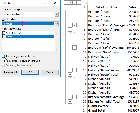
We call the menu «Subtotals» again. We remove the tick «Replace current subtotals», and in the «Use function:» field, select «Average».
Formula «Subtotals» in Excel: the examples
The «INTERMEDIATE» function returns the subtotal in the list or in the database. Syntax: the number of function, the reference 1; the reference 2;…
The number of function — is a number from 1 to 11, which shows the statistical function for calculating subtotals:
- AVERAGE (the average arithmetic)
- ACCOUNT (the number of cells)
- COUNTAIN (the number of non-empty cells)
- MAX (maximum value in the range)
- MIN (the minimum value)
- COMPOS (product of numbers)
- STDEV (standard deviation from the sample)
- STDEVP (standard deviation of the population)
- SUM
- DISP (variance in production)
- DISPP (population variance)
The reference 1 – is the mandatory argument indicating the named range for finding the subtotals.
The features of the «work» function:
- outputs the result by explicit and hidden lines;
- excludes lines not included in the filter;
- counts only in columns, for rows not suitable.
Consider using the function as an example:
- Create the additional line for displaying subtotals. For example, there is «Sum of selected values».
- Turn on the filter. Let’s leave in the table only the data on the value of the Kitchen «Amaids».
- In the cell B2 we introduce the formula =SUBTOTAL():
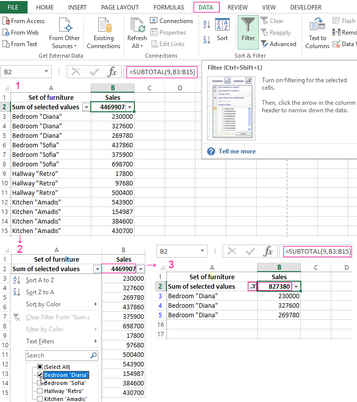
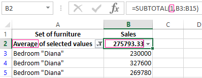
The formula for the average value of the intermediate total of the range:
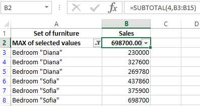
The formula for the maximum value (for bedrooms):
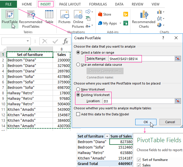
Subtotals in the Excel Pivot Table
In the summary table, you can show or hide subtotals for rows and columns.
- The automatic summation function for calculation of totals is already included the formation of the consolidated report.
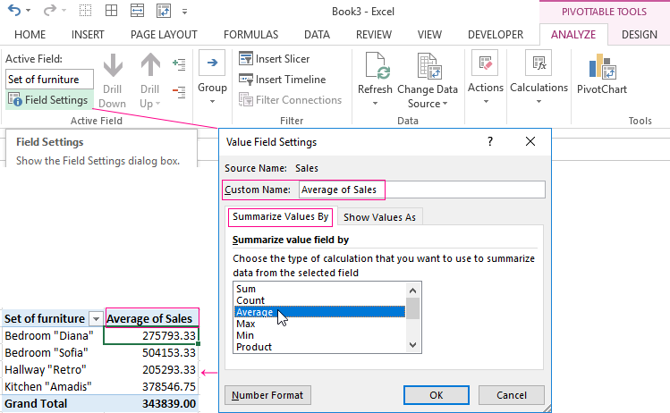
- To apply another function, in the «PIVOTTABLE TOOL» section on the «ANALYZE» tab, we find the «Active Field» group. The cursor must be in the cell of the column whose values the function will be applied to. Press the button «Field Setting». In the menu that opens, select «Average». Assign the desired function to the subtotals.
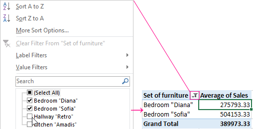
- To display totals for individual values, use the filter button in the right corner of the name of column.
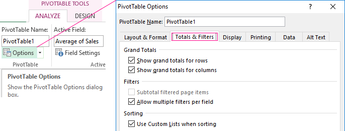
In the «PIVOTTABLE TOOL» menu «ANALYZE»-«PivotTable»-«Options», the «Totals and Filters» tab is available.
Download examples of subtotals
Thus, to display subtotals in Excel lists, three methods are used: the command of the «DATA»-«Outline» group, the built-in function and the summary table.
Returns an aggregate result for data provided
What is the SUBTOTAL Function in Excel?
The SUBTOTAL Function[1]in Excel allows users to create groups and then perform various other Excel functions such as SUM, COUNT, AVERAGE, PRODUCT, MAX, etc. Thus, the SUBTOTAL function in Excel helps in analyzing the data provided.
Formula
SUBTOTAL = (method, range1, [range2 …range_n])
Where method is the type of subtotal you wish to obtain
Range1,range2…range_n is the range of cells you wish to subtotal
Why do we need to use SUBTOTALS?
Sometimes, we need data based on different categories. SUBTOTALS help us to get the totals of several columns of data broken down into various categories.
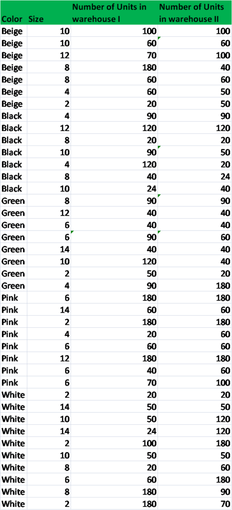
For example, let’s consider garment products of different sizes manufactured. The SUBTOTAL function will help you to get a count of different sizes in your warehouse.
To learn more, launch our free Excel crash course now!
How to use the SUBTOTAL Function in Excel?
There are two steps to follow when we wish to use the SUBTOTAL function. These are:
- Formatting and sorting of the provided Excel data.
- Applying SUBTOTAL to the table.
Let’s understand this Excel function with the help of an example. We use data provided by a garment manufacturer. He manufactures T-shirts of five different colors, i.e., White, Black, Pink, Green, and Beige. He produces these T-shirts in seven different sizes, i.e. 2, 4, 6, 8, 10, 12, 14. The relevant data are below:
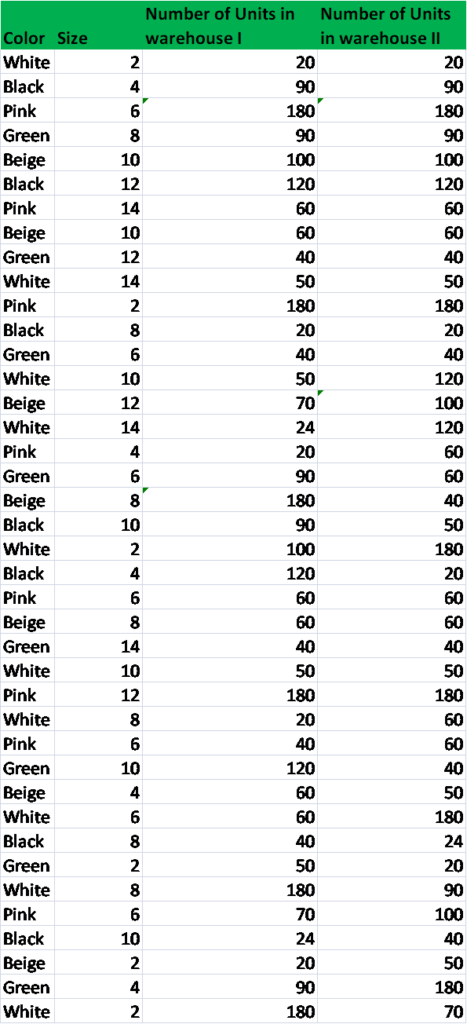
The warehouse manager provides random data. Now for the analysis, we need to get the total number of T-shirts of each color lying in the warehouse.
Step 1
First, we need to sort the worksheet on the basis of data we need to subtotal. As we need to get the subtotals of T-shirts by colors, we will sort it accordingly.
To do that, we can use the SORT function under the Data tab.
Step 2
The next step would be to apply the SUBTOTAL function. This can be done as shown below:
Select the Data tab, and click on SUBTOTAL.
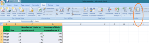
When we click on it, the Subtotal dialogue box will appear as shown below:
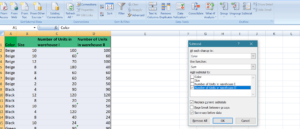
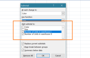
Now, click the drop-down arrow for the “At each change in: field.” We can now select the column we wish to subtotal. In our example, we’ll select Color.
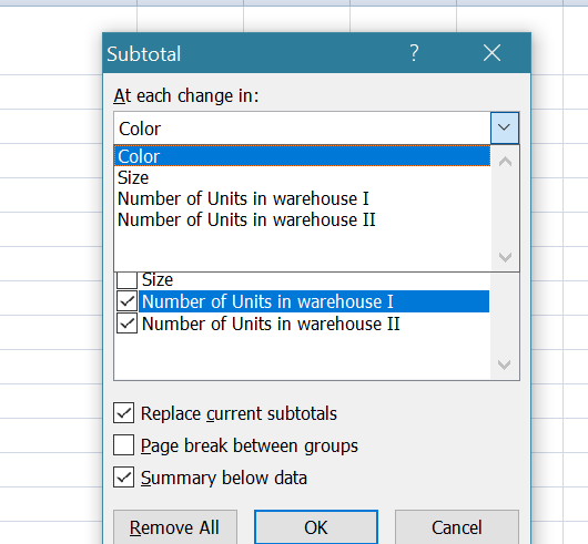
Next, we need to click the drop-down arrow for the “Use function: field.” This will help us select the function we wish to use. There are 11 available functions. We need to choose depending on our requirements. In our example, we’ll select SUM to find out the total number of T-shirts lying in each warehouse.

Next, we move to “Add subtotal to: field.” Here we need to select the column where we require the calculated subtotal to appear. In our example, we’ll select Number of Units in Warehouse I and Warehouse II.
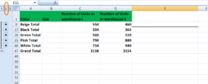
After that, we need to click OK and we will get the following results:

As we can see in the screenshot above, the subtotals are inserted as new rows below each Group. When we create subtotals, our worksheet is divided into different levels. Depending on the information you wish to display in the worksheet, you can switch between these levels.
The level buttons in our example are images of buttons for Levels 1, 2, 3, which can be seen on the left side of the worksheet. Now suppose I just want to see the total T-shirts lying in the warehouse of different colors, we can click on Level 2.
If we click on the highest level (Level 3), we will get all the details.
To learn more, launch our free Excel crash course now!
Tips for the SUBTOTAL function:
Tip #1
Let’s assume, we wish to ensure that all colors of T-shirts are available in all sizes in either of the warehouses. We can follow these steps:
Step 1: Click on Subtotal. Remember we are adding one more criterion to our current Subtotal data.
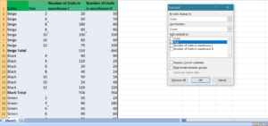
Now,
Step 2: Select COUNT from the drop-down menu, and Size from the “Add subtotal field to.” After that, uncheck the “Replace current subtotals.” Once you click OK, you will get the following data:
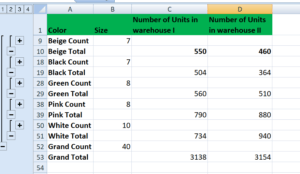
This will help us ensure that the count for different sizes and we can sort data in such a manner that the repetitions are not there.
Tip #2
Always sort data by column we will use to subtotal.
Tip #3
Remember that each column we wish to subtotal includes a label in the first row.
Tip #4
If you wish to put a summary of the data, uncheck the box “Summary below the data when inserting Subtotal.”
Free Excel Course
Check out our Free Excel Crash Course to learn more about Excel functions using your own personal instructor. Master Excel functions to create more sophisticated financial analysis and modeling towards building a successful career as a financial analyst.
Additional Resources
Thanks for reading CFI’s guide to important Excel functions! By taking the time to learn and master these functions, you’ll significantly speed up your financial analysis. To learn more, check out these additional CFI resources:
- Excel Functions for Finance
- Advanced Excel Formulas Course
- Advanced Excel Formulas You Must Know
- Excel Shortcuts for PC and Mac
- See all Excel resources