
A perceiver’s job in spoken word recognition is to use the data from their senses to decide which of the hundreds of words they know best fits the context. After 40 years of study, it is generally agreed that we recognize words via an engagement and competition process, with more frequently used terms receiving preference. Modern speech recognition models all use this procedure. However, the specifics may differ.
Explaining Spoken Word Recognition
Listeners with normal hearing can quickly and seemingly effortlessly adjust to various variations in the speech signal and the immediate listening environment. Strong SWR relies on early sensory processing and storage of language into lexical representations. However, the robust character of SWR cannot be fully accounted for by audibility and sensory processing, particularly in compromised listening environments. , researchers provide a background on the subject, cover some key theoretical concerns, and then examine some modern models of SWR. Finally, we highlight some exciting new avenues to pursue and hurdles to overcome, such as the ability of deaf youngsters with cochlear implantation, bilinguals, and elderly persons to understand speech with an accent.
Recently Developed Speech Recognition Models
Word recognition systems function best when they can dependably pick out the word whose lexical representation is most similar to the input representation. Even though this may seem obvious, a recognition system that merely compared the perceptual input to each lexical entry and picked the one with the best fit would be the best way to perform isolated word recognition without the interference of higher-level contextual constraints.

Track Down
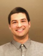
Trace model is a localist fully convolutional model of spoken word recognition based on interactive activation, with three tiers of nodes representing feature representations, phoneme representations, and word representations, respectively. Loyalist versions of word recognition treat allophones, phonemes, and words as discrete units. The processing units in Trace are interconnected by excitatory and inhibitory pathways, respectively, to increase and decrease unit activation in response to incoming stimuli and system activity.
Parsyn
The Parsyn model is a regionalist connectionist architecture with three tiers of linked units: input allophone, pattern allophone, and word. Within a level, connections between units are antagonistic to one another. However, linking respondents’ need to answer units at the design level is helpful in both directions.
Method for Analyzing Cohorts in a Distributed Setting
In the OCM (distributed cohort model), the activation associated with a word is spread among many low-level processors. The speech-based featural input is projected onto the basic semantic and phonological elements. Due to the decentralized nature of the OCM, no intermediary or sublexical representation elements can be found in the OCM. As a bonus, in contrast to the localist models’ reliance on a method of lateral inhibition, the lexical rivalry is depicted as a blending of multiple consistent lexical elements based on bottom-up input.
Activation-Competition Models
When put into perspective, the new batch of activation-competition systems has rather modest distinctions. According to all, multiple activation and rivalry among form-based lexical components define spoken word recognition. The fundamentals have been established, even though the particulars may differ. Segmentation, vocabulary, the type of lexical feedback, the significance of context, and so on are only a few of the phenomena that the models attempt to explain. Given the fundamental similarities of the existing models, it seems unlikely that these issues would ultimately determine which model should win out.

Referential Variation and Processing
Spoken word processing is significantly affected by subtle differences in the presentation of acoustic stimuli. Pisani (1992) as the first researchers to examine the processing costs associated with talker variability (a kind of indexical variation) Peters examined the differences in the clarity of single-talker and multi-talker transmissions in the presence of background noise. He discovered that one-on-one conversations were consistently easier to understand than group chats.
Phonological Shifts in Allophony
The present state of speech recognition models is inadequate when accounting for individual differences in pronunciation. Scientific studies on how indexical diversity in speech recognition is represented and processed provide weight to our argument. New research on allophonic variance points to gaps in the existing models. Allophonic variance refers to effective passive and acoustic differences among vocal stations belonging to the same phonics category insights into the possible shortcomings of present modeling methodologies have been provided by recent studies of allophonic variance.
Edges Activate Phonetic Counterparts
This finding defies capture by any existing computer model spoken or word recognition. For instance, the discovery that flaps trigger their phonemic counterparts dictates that, at a minimum, both Trace and Shortlist should include an allophonic layer of representation. Allophonic support is unique to PARSYN. On the other hand, PARSYN’s absence of phonemic representations may make it difficult to account for the activation of so. Some mediated access theories may also explain the observation that core representations are engaged. However, these theories need to explain the time course of cognition, specifically why the impacts of representations disappear when answers are fast. Finally, while the DCM may account for cases in which underlying models become deactivated, it will likely need help to emulate cases in which processing is impeded. For the umpteenth time, the current models cannot handle the pressure of variance.
Conclusion
Fundamental complications are presented by variance, requiring a rethinking of our models’ representational systems. New information points to the existence simultaneously as forms that contain both the concrete and the general. Furthermore, we need to imagine systems in which the processing of the particular and the general follows a time course that is predictable and represents the underlying design of the processing system. Last but not least, the next wave of models we develop will need to account for the malleable character of human perception. The adult brain seems capable of fine and frequent tuning in response to external input. Models of recognition that do justice to the subject need to include control conditions that can take into account the ability to adapt to perception, which will undoubtedly have far-reaching consequences for the structure and design of the representational system.
Such accounts of SWR assume that highly detailed stimulus information in the speech signal and listening environment is encoded, processed, and stored by the listener and subsequently becomes an inseparable component of rich and highly detailed lexical representations of spoken words (Port, 2010a, 2010b).
From: Neurobiology of Language, 2016
Spoken Word Recognition
David B. Pisoni, Conor T. McLennan, in Neurobiology of Language, 2016
The most distinctive hallmark of human spoken word recognition (SWR) is its perceptual robustness to the presence of acoustic variability in the transmission and reception of the talker’s linguistic message. Normal-hearing listeners adapt rapidly with little apparent effort to many different sources of variability in the speech signal and their immediate listening environment. Sensory processing and early encoding of speech into lexical representations are critical for robust SWR. However, audibility and sensory processing are not sufficient to account for the robust nature of SWR, especially under degraded listening conditions. In this chapter, we describe the historical roots of the field, present a selective review of the principle theoretical issues, and then consider several contemporary models of SWR. We conclude by identifying promising new directions and future challenges, including the perception of foreign accented speech, SWR by deaf children with cochlear implants, bilinguals, and older adults.
Read full chapter
URL:
https://www.sciencedirect.com/science/article/pii/B9780124077942000201
Computational Psycholinguistics
R. Klabunde, in International Encyclopedia of the Social & Behavioral Sciences, 2001
3.2 Computer Models of Language Comprehension
Since comprehension begins with the recognition of words, this section deals first with models of spoken word recognition. In spoken word recognition, the models proposed must answer two main questions. First, they must describe how the sensory input is mapped onto the lexicon, and second, what the processing units are in this process.
The Trace model (McClelland and Elman 1986) is an interactive model that simulates how a word will be identified from a continuous speech signal. The problem with this task is that continuity of the signal does not provide clear hints about where a word begins and where it ends. By means of activation spreading through a network that consists of three layers (features, phonemes, and words), the system generates competitor forms, converging to the ultimately selected word. Competition is realized by inhibitory links between candidates.
The Shortlist model (Norris 1994) is based on a modular architecture with two distinct processing stages. It uses spreading activation as well, but in a strictly bottom-up way. Contrary to Trace, it generates a restricted set of lexical candidates during the first stage. During the second stage, the best fitting words are linked via an activation network.
Both models account for experimental data on the time course of word recognition. Assumptions on the direction of activation flow and its nature lead to several differing predictions, but the main different prediction concerns lexical activation. While Trace assumes that a very large number of items are activated, Shortlist assumes that a much smaller set of candidates is available so that the recognition of words beginning at different time points is explained differently.
The last model is a model of sentence processing. In sentence processing, one of the fundamental questions is why certain sentences receive a preferred syntactic structure and semantic interpretation.
The Sausage Machine (Fodor and Frazier 1980) is a parsing model that assumes two stages in parsing with both stages having a limited working capacity. The original idea behind the model is to explain preferences in syntactic processing solely on the architectural basis by means of the limitations in the working memories.
The Sausage Machine is a quasi-deterministic model, because one syntactic structure for each sentence is generated. Only if the analysis turns out to be wrong, is a reanalysis performed. Since reanalyzing a sentence is a time consuming process, the system tries to avoid this whenever possible. The model accounts for garden path effects and the difficulty in understanding multiple center embedded sentences (like ‘the house the man sold burnt down’). Furthermore, the model explains interpretation preferences by means of the limitation in working memories. However, it is now understood that the architecture of a system cannot be the only factor that is responsible for processing preferences, but additional parsing principles must be assumed (Wanner 1980). Newer computational models of sentence processing show that an explanation of several phenomena in sentence processing requires the early check of partial syntactic structures with lexical and semantic knowledge (Hemforth 1993).
Read full chapter
URL:
https://www.sciencedirect.com/science/article/pii/B0080430767005428
The Temporal Lobe
Delaney M. Ubellacker, Argye E. Hillis, in Handbook of Clinical Neurology, 2022
Conclusions
Lesion studies show that specific regions of the left (or bilateral) temporal cortex are associated with distinct impairments in object recognition, spoken word comprehension, naming, reading, and spelling. These areas are thought to be critical nodes in networks of the brain that link various forms of input to meaning and to output. Although the nodes work together as neural networks, damage to different nodes results in distinct language deficits. Studies of functional and structural imaging are beginning to reveal how these cortical nodes and associated white matter tracts work together to support language functions.
Read full chapter
URL:
https://www.sciencedirect.com/science/article/pii/B9780128234938000134
Word Recognition
J. Zevin, in Encyclopedia of Neuroscience, 2009
Superior Temporal Gyrus and Superior Temporal Sulcus
Superior temporal gyrus (STG) is the site of auditory association cortex (and a site of multisensory integration) and thus necessarily plays some role in spoken word recognition. Evidence that its role extends beyond that of higher-level perceptual processing was found as early as 1871 by Karl Wernicke. He discovered that lesions in the posterior portion of the left STG were associated with the loss of the ability to comprehend and produce spoken words. More recently, it has been found that this phenomenon of ‘Wernicke’s aphasia’ is observed to result from brain damage to a broad variety of sites; furthermore, damage to traditional Wernicke’s area does not always result in aphasic symptoms.
Neuroimaging studies of healthy subjects have found evidence for a role in processing of word meanings for both anterior and posterior STG as well as superior temporal sulcus (STS; the sulcus that divides the STG from the middle temporal gyrus). The STS, in particular, responds more strongly to interpretable speech than to a range of stimuli matched on lower level acoustic dimensions. The STS is also a likely site of integration between print and sound in visual word recognition.
Read full chapter
URL:
https://www.sciencedirect.com/science/article/pii/B9780080450469018817
The Neurobiology of Lexical Access
Matthew H. Davis, in Neurobiology of Language, 2016
44.5 Conclusion
This chapter has presented a tripartite account of the brain regions that support lexical processing of spoken words. The functional goals of three temporal lobe systems have been introduced in the context of key computational challenges associated with spoken word recognition. First, listeners must integrate current speech sounds with previously heard speech in recognizing words. This motivates a hierarchy of representations that temporally integrate speech signals over time localized to anterior regions of the STG. A second challenge is that for listeners to repeat degraded words correctly requires that they recover the speakers’ intended articulatory gestures. The tripartite account localizes this process to auditory-motor links mediated by TPJ regions and proposes that these links play a key role in supporting robust identification and perceptual learning of degraded spoken words. The third challenge relates to extracting meaning from spoken words, which is proposed to be supported by cortical areas in posterior ITG and surrounding regions (MTG and fusiform). Despite the three-way functional segregation that is at the heart of this triparate account, this chapter also acknowledges that reliable recognition of familiar words, optimally efficient processing of incoming speech, and learning of novel spoken words all depend on combining information between these processing pathways. This is achieved through convergent connectivity within the lateral temporal lobe, in frontal or medial temporal regions, and through top-down predictions mapped back to peri-auditory regions of the STG. A key goal for future research must be to specify these convergent mechanisms in more detail and derive precise computational proposals for how the tripartite lexical system supports the everyday demands of human speech comprehension.
Read full chapter
URL:
https://www.sciencedirect.com/science/article/pii/B9780124077942000444
Language in Aged Persons
E.A.L. Stine-Morrow, M.C. Shake, in Encyclopedia of Neuroscience, 2009
Word processing
Vocabulary often shows an increase with age, particularly among those who read regularly. Word recognition appears to be highly resilient through late life. For example, word frequency effects (i.e., faster processing for more familiar words) in reading and word naming are typically at least as large for older adults as they are for young. Sublexical features (e.g., neighborhood density), however, may have a smaller effect on processing time on older readers, suggesting that accumulated experience with literacy may increase the efficiency of orthographic decoding.
By contrast, declines in auditory processing can make spoken word recognition more demanding so that more acoustic information is needed to isolate the lexical item. Such effects may not merely disrupt encoding of the surface form but also tax working memory resources that would otherwise be used to construct a representation of the text’s meaning. For example, when elders with normal or impaired hearing listen to a word list and are interrupted periodically to report the last word heard, they may show negligible differences. However, if asked to report the last three words, hearing-impaired elders will likely show deficits. The explanation for such a provocative finding is that the hearing-impaired elders overcome a sensory loss at some attentional cost so as to exert a toll on semantic and elaborative processes that enhance memory. Presumably, the same mechanisms would operate in ordinary language processing.
At the same time, there is evidence that older adults can take differential advantage of context in the recognition of both spoken and written words, especially in noisy environments. Semantic processes at the lexical level also appear to be largely preserved. Semantic priming effects (i.e., facilitation in word processing by prior exposure to a related word) are typically at least as large among older adults as among the young. Also, in the arena of neurocognitive function, evoked potentials show similar lexical effects for young and old – a reduced N400 component for related words relative to unrelated controls. One area of difficulty that older adults may have in word processing is in deriving the meaning of novel lexical items from context, with research showing that older adults are likely to infer more generalized and imprecise meanings relative to the young – a difference that can be largely accounted for in terms of working memory deficits.
Read full chapter
URL:
https://www.sciencedirect.com/science/article/pii/B9780080450469018726
Word Recognition, Cognitive Psychology of
M.A. Moreno, G.C. van Orden, in International Encyclopedia of the Social & Behavioral Sciences, 2001
2 Word Recognition as Information Processing
The logic of the additive factors method also fits the metaphor of cognition as information processing. For the chain of dominoes, substitute the guiding analogy of a flow chart of information processing, like unidirectional flow charts of computer programs. Information flows from input (stimulus) to output (behavior) through a sequence of cognitive components. In word recognition, input representations from a sensory process—visual or auditory features of a word—are transformed into an output representation—the identity of the word—that, in turn, becomes the input representation for a component downstream (i.e., a component of response production or sentence processing). In this tradition, empirical studies of word recognition pertain to the structure and function of the lexicon. The lexicon is a memory component, a mental dictionary, containing representations of the meanings, spellings, pronunciations, and syntactic functions of words. Structure refers to how the word entries are organized, and function refers to how words are accessed in, or retrieved from, the lexicon. Two seminal findings illustrate the distinction: semantic priming effects and word frequency effects. Both effects are found in lexical decision performance.
2.1 The Lexical Decision Task
In the lexical decision task, a person is presented, on each trial, with a target string of letters, and must judge whether the target string is a correctly spelled word in English (or some other reference language). Some trials are catch trials, which present nonwords such as ‘glurp.’ (One may also present words and nonwords auditorally, to examine spoken word recognition.) The participant presses a ‘word’ key to indicate a word and a ‘nonword’ key otherwise. The experimenter takes note of the response time, from when the target stimulus appeared until the response key is pressed, and whether the response was correct. Response time and accuracy are the performance measures.
2.2 Semantic Priming and the Structure of the Lexicon
Word pairs with related meanings, such as ‘doctor’ and ‘nurse’ or ‘bread’ and ‘butter,’ produce semantic priming effects. Semantic priming was discovered by David Meyer and Roger Schvaneveldt, working independently (they chose to report their findings together). Lexical decision performance to a word is improved by prior presentation of its semantically related word. Prior recognition of ‘doctor,’ as a word, facilitates subsequent recognition of ‘nurse’; lexical decisions to ‘nurse’ are faster and more accurate, compared with a control condition. This finding is commonly interpreted to mean that semantically related words are structurally connected in the lexicon, such that retrieval of one inevitably leads to retrieval of the other (in part or in whole).
2.3 Word Frequency and the Function of Lexical Access
Word frequency is estimated using frequency counts. The occurrence of each word, per million, is counted in large samples of text. Lexical decision performance is correlated with word frequency. Words that occur more often in text (or in speech) are recognized faster and more accurately than words that occur infrequently. This finding is interpreted in a variety of ways. The common theme is that lexical access functions in a manner that favors high-frequency words. In one classical account, proposed by John Morton, access to a lexical entry is via a threshold. Word features may sufficiently activate a lexical entry, to cross its activation threshold, and thus make that entry available. Common, high-frequency words have lower threshold values than less common words. In a different classical account, proposed by Kenneth Forster, the lexicon is searched in order of word frequency, beginning with high frequency words.
2.4 Challenges to the Information Processing Approach
Additive interaction effects are almost never observed in word recognition experiments, and, while it is not possible to manipulate all word factors simultaneously in one experiment, it is possible to trace chains of nonadditive interactions across published experiments that preclude the assignment of any factors to distinct components. Moreover, all empirical phenomena of word recognition appear to be conditioned by task, task demands, and even the reference language, as the examples that follow illustrate.
The same set of words, which produce a large word frequency effect in the lexical decision task, produce a reduced or statistically unreliable word frequency effect in naming and semantic categorization tasks. All these tasks would seem to include word recognition, but they do not yield the same word recognition effects. Also, within the lexical decision task, itself, it is possible to modulate the word frequency effect by making the nonwords more or less word-like (and, in turn, to modulate a nonadditive interaction effect between word frequency and semantic priming). Across languages, Hebrew produces a larger word frequency (familiarity) effect than English, and English than Serbo–Croation.
Consider the previous examples together, within the guidelines of additive factors logic. Word recognition factors cannot be individuated from each other, and they cannot be individuated from the context of their occurrence (task, task demands, and language). The limitations of additive factors method are well known. Because additivity is never consistently observed, we have no empirical basis for individualizing cognitive components. The de facto practice in cognitive psychology is to assume that laboratory tasks and manipulations may differ from each other by the causal equivalent of one component (‘one domino’). But how does one know which tasks or manipulations differ by exactly one component? We require a priori knowledge of cognitive components, and which components are involved in which laboratory tasks, to know reliably which or how many components task conditions entail. Notice this circularity, pointed out by Robert Pachella: the goal is to discover cognitive components in observed laboratory performance, but the method requires prior knowledge of the self same components.
Despite these problems, most theorists share the intuition that a hypothetical component of word recognition exists. When intuitions diverge, however, there may be no way to reconcile differences. Theorists who assume that reading is primarily an act of visual perception discover a visual component of word recognition; theorists who assume that reading is primarily a linguistic process discover a linguistic component of word recognition, in the same performance phenomena. Repeated contradictory discoveries, in the empirical literature, have lead to a vast debate concerning which task conditions provide an unambiguous view of word recognition in operation. The debate hinges on exclusionary criteria that may correctly exclude task effects and bring word recognition into clearer focus. Otherwise, inevitably, one laboratory’s word recognition effect is another laboratory’s task artifact.
Read full chapter
URL:
https://www.sciencedirect.com/science/article/pii/B0080430767015539
Language and Aging☆
Matthew C. Shake, Elizabeth A.L. Stine-Morrow, in Reference Module in Neuroscience and Biobehavioral Psychology, 2017
Word Processing
Vocabulary often shows an increase with age, particularly among those with well-developed and sustained literacy practices. Word recognition appears to be highly resilient through late life. For example, word frequency effects (i.e., faster processing for more familiar words) in reading and word naming are typically at least as large for older adults as they are for young. Sublexical features (e.g., neighborhood density, a measure of how similar a word is to other words in the language), however, may have a smaller effect on processing time on older readers, suggesting that accumulated experience with literacy may increase the efficiency of orthographic decoding.
By contrast, declines in auditory processing can make spoken word recognition more demanding so that more acoustic information is needed to isolate the lexical item. Such effects may not merely disrupt encoding of the surface form but also tax working memory resources that would otherwise be used to construct a representation of the text’s meaning. For example, when elders with normal or impaired hearing listen to a word list and are interrupted periodically to report the last word heard, they may show negligible differences. However, if asked to report the last three words, hearing-impaired elders will likely show deficits. The explanation for such a provocative finding is that the hearing-impaired elders overcome a sensory loss at some attentional cost so as to exert a toll on semantic and elaborative processes that enhance memory. Presumably, the same mechanisms would operate in ordinary language processing.
At the same time, there is behavioral evidence that older adults can take differential advantage of context in the recognition of both spoken and written words, especially in noisy environments. Semantic processes at the lexical level also appear to be largely preserved. Semantic priming effects (i.e., facilitation in word processing by prior exposure to a related word) are typically at least as large among older adults as among the young. Also, in the arena of neurocognitive function, electrophysiological data show that some kinds of stimulus-evoked changes in brain potentials (known as event-related brain potentials, or ERPs) are similar in young and old for words presented in isolation; for example, a reduced “N400 component” (a negative shift in waveform amplitude occurring approximately 400 ms after word presentation) for predictable relative to unpredictable words. However, older adults tend to show this effect to a much reduced degree, suggesting that activation of meaning features as the text unfolds may be more constrained among older adults relative to the young. Older adults with higher verbal fluency, on the other hand, appear better able to engage in anticipatory language processing as younger adults do. A puzzle that remains is to reconcile the electrophysiological data suggesting that older adults are less likely to use predictive processing to isolate words from context with behavioral data showing enhanced contextual facilitation with age.
Read full chapter
URL:
https://www.sciencedirect.com/science/article/pii/B9780128093245018897
Processing Tone Languages
Jackson T. Gandour, Ananthanarayan Krishnan, in Neurobiology of Language, 2016
87.4 Tonal Versus Segmental Units
Linguistic theory informs us that the onset and rime of a syllable contain segmental units. They differ in their duration and the order in which their information unfolds in time over the duration of a syllable. Rimes and tones, however, overlap substantially in the order in which their information unfolds in time. Tones are suprasegmental; they are mapped onto (morpho)syllables.
Depending on task demands, tones elicit effects that differ from those of segments. The time course and amplitude of N400 (a negative component associated with lexical semantic processing that peaks approximately 400 ms after the auditory stimulus) were the same for consonant, rime, and tone violations in Cantonese (12: Schirmer, Tang, Penney, Gunter, & Chen, 2005). Their findings were replicated in Mandarin, but syllable violations elicited an earlier and stronger N400 than tone (17: Malins & Joanisse, 2012; cf. 16: Zhao, Guo, Zhou, & Shu, 2011). This separation of tone from its carrier syllable was also reported in an auditory verbal recognition paradigm in which subjects selectively attended to either the syllable or the tone (10: Li et al., 2003). In a spoken word recognition paradigm, tones elicited larger late positive event-related potential (ERP) component than vowels (19: Hu, Gao, Ma, & Yao, 2012). In a left brain-damaged Chinese aphasic, vowels were spared and tones were severely impaired (11: Liang & van Heuven, 2004). These findings together support a functional dissociation of tonal and segmental information.
It is well-known that hemispheric specialization may be driven by differences in acoustic features associated with segments. The question is whether hemispheric specialization for tone can be dissociated from segments. Tones induce greater activation in the right posterior middle frontal gyrus (MFG) for English speakers when compared with consonants or rimes (9: Gandour et al., 2003). This area has been implicated in pitch perception (Zatorre et al., 2002). Their increased activation is presumably due to their lack of experience with Chinese tones. Using a tone identification task, the right IFG was found to be activated in English learners of Mandarin tone only after training (Wang, Sereno, Jongman, & Hirsch, 2003). This finding demonstrates early cortical effects of learning a second language that involve recruitment of cortical regions implicated in tonal processing. Focusing on hemispheric specialization for tone production (14: Liu et al., 2006), Mandarin tones elicited more activity in the right IFG than vowels. This rightward preference for tonal processing converges more broadly with the role of the RH in mediating speech prosody (Friederici & Alter, 2004; Glasser & Rilling, 2008; Wildgruber, Ackermann, Kreifelts, & Ethofer, 2006).
As measured by the mismatch negativity (MMN), a fronto-centrally distributed cortical ERP that indexes a change in auditory detection, it is well-known that language experience may influence the automatic, involuntary processing of consonants and vowels (Naatanen, 2001, review). Therefore, one would expect language experience to modulate the automatic cortical processing of lexical tones. Tones evoked stronger MMN in the RH relative to the LH, whereas consonants produced the opposite pattern (13: Luo et al., 2006). An fMRI study showed that Mandarin tones, relative to consonants or rimes, elicited increased activation in right frontoparietal areas (15: Li et al., 2010). Taken together, these data suggest the balance of hemispheric specialization may be modulated by distinct acoustic features associated with tonal as compared with segmental units.
Read full chapter
URL:
https://www.sciencedirect.com/science/article/pii/B9780124077942000870
Neural Networks and Related Statistical Latent Variable Models
M.A. Tanner, R.A. Jacobs, in International Encyclopedia of the Social & Behavioral Sciences, 2001
1 Introduction
This article presents statistical features associated with artificial neural networks, as well as two other related models, namely mixtures-of-experts and hidden Markov models.
Historically, the study of artificial neural networks was motivated by attempts to understand information processing in biological nervous systems (McCulloch and Pitts 1943). Recognizing that the mammalian brain consists of very complex webs of interconnected neurons, artificial neural networks are built from densely interconnected simple processing units, where each unit receives a number of inputs and produces a single numerical output. However, while artificial neural networks have been motivated by biological systems, there are many aspects of biological systems not adequately modeled by artificial neural networks. Indeed, many aspects of artificial neural networks are inconsistent with biological systems. Though the brain metaphor provides a useful source of inspiration, the viewpoint adopted here is that artificial neural networks are a general class of parameterized statistical models consisting of interconnected processing units.
Artificial neural networks provide a general and practical approach for approximating real-valued (regression problems) and discrete-valued (classification problems) mappings between covariate and response variables. These models, combined with simple methods of estimation (i.e., learning algorithms), have proven highly successful in such diverse areas as handwriting recognition (LeCun et al. 1989), spoken word recognition (Lang et al. 1990), face recognition (Cottrell 1990), text-to-speech translation (Sejnowski and Rosenberg 1986), and autonomous vehicle navigation (Pomerleau 1993).
An artificial neural network consists of multiple sets of units: one set of units corresponds to the covariate variables, a second set of units corresponds to the response variables, and a third set of units, referred to as hidden units, corresponds to latent variables. The hidden units (or, more precisely, their associated hidden or latent variables) mediate the nonlinear mapping from covariate to response variables. Based on observed pairings of covariate and response variables, the back-propagation algorithm is commonly used to estimate the parameters, called weights, of the hidden units.
Some mixture models have statistical structures that resemble those of artificial neural networks. Mixture models are multiple-component models in which each observable data item is generated by one, and only one, component of the model. Like artificial neural networks, mixture models also contain latent or hidden variables. The hidden variables of a mixture model indicate the component that generated each data item.
Mixtures-of-experts (ME) models combine simple conditional probability distributions, such as unimodal distributions, in order to form a complex (e.g., multimodal) conditional distribution of the response variables given the covariate variables. They combine properties of generalized linear models (McCullagh and Nelder 1989) with those of mixture models. Like generalized linear models, they are used to model the relationship between covariate and response variables. Typical applications include nonlinear regression and binary or multiway classification. However, unlike standard generalized linear models they assume that the conditional distribution of the responses is a finite mixture distribution. Mixtures-of-experts are ‘piecewise estimators’ in the sense that different mixture components summarize the relationship between covariate and response variables for different subsets of the observable data items. The subsets do not, however, have hard boundaries; a data item might simultaneously be a member of multiple subsets. Because ME assume that the probability of the response variables given the covariate variables is a finite mixture distribution, they provide a motivated alternative to nonparametric models such as artificial neural networks, and provide a richer class of distributions than standard generalized linear models.
Hidden Markov models (HMMs), in contrast with ME models, do not map covariate to response variables; instead, they are used to summarize time-series data. To motivate HMMs, consider the following scenario (Rabiner 1989). A person has three coins. At each time step, she performs two actions. First, she randomly selects a coin by sampling from a multinomial distribution. The parameters of this distribution are a function of the coin that was selected at the previous time step. Next, the selected coin is flipped in order to produce an outcome. Each coin has a different probability of producing either a head or a tail. A second person only observes the sequence of outcomes. Based on this sequence, the person constructs a statistical model of the underlying process that generated the sequence. A useful statistical model for this scenario is a hidden Markov model.
HMMs are mixture models whose components are typically members of the exponential family of distributions. It is assumed that each data item was generated by one, and only one, of the components. The dependencies among the data items are captured by the fact that HMMs include temporal dynamics which govern the transition from one component to another at successive time steps. More specifically, HMMs differ from conventional mixture models in that the selection of the mixture component at time step t is based upon a multinomial distribution whose parameters depend on the component that was selected at time step t−1. HMMs are useful for modeling time series data because they explicitly model the transitions between mixture components, or states as they are known in the engineering literature. An advantage of HMMs is that they can model data that violate the stationarity assumptions characteristic of many other types of time series models. The states of the HMM would be Bernoulli distributions in the above scenario. More commonly HMMs are used to model sequences of continuous signals, such as speech data. The states of an HMM would be Gaussian distributions in this case.
Artificial neural networks and mixture models, such as mixtures-of-experts and hidden Markov models, can be seen as instances of two ends of a continuum. Artificial neural networks are an example of a ‘multiple-cause’ model. In a multiple-cause model, each data item is a function of multiple hidden variables. For instance, a response variable in a neural network is a function of all hidden variables. An advantage of multiple-cause models is that they are representationally efficient. If each hidden variable has a Bernoulli distribution, for example, and if one seeks N bits of information about the underlying state of a data item, then a model with N latent variables is sufficient. In the case when there is a linear relationship between the latent and observed variables, and when the variables are Gaussian distributed, such as is the case with factor models, then the equations for statistical inference (i.e., the determination of a probability distribution for the hidden variables given the values of the observed variables) are computationally efficient. However, a disadvantage of multiple-cause models is that inference tends to be computationally intractable when there is a nonlinear relationship between latent and observed variables, as is frequently the case with neural networks.
Consequently, researchers also consider ‘single-cause’ models, such as mixture models. Mixture models are regarded as instances of single-cause models due to their assumption that each observable data item was generated by one, and only one, component of the model. An advantage of this assumption is that it leads to a set of equations for performing statistical inference that is computationally efficient. A disadvantage of this assumption is that it makes mixture models inefficient from a representational viewpoint. Consider, for example, a two-component mixture model where each component is a Gaussian distribution. This model provides one bit of information regarding the underlying state of a data item (either the data item was sampled from the first Gaussian distribution or it was sampled from the second Gaussian distribution). Suppose that one seeks N bits of information about the underlying state of a data item. A mixture model requires 2N components in order to provide this amount of information. That is, as the amount of information grows linearly, the number of required components grows exponentially.
As discussed at the end of this article, a recent trend in the research literature is to consider novel statistical models that are not purely single-cause and are not purely multiple-cause, but rather combine aspects of both.
Read full chapter
URL:
https://www.sciencedirect.com/science/article/pii/B0080430767004307
What is speech recognition?
Speech recognition, or speech-to-text, is the ability of a machine or program to identify words spoken aloud and convert them into readable text. Rudimentary speech recognition software has a limited vocabulary and may only identify words and phrases when spoken clearly. More sophisticated software can handle natural speech, different accents and various languages.
Speech recognition uses a broad array of research in computer science, linguistics and computer engineering. Many modern devices and text-focused programs have speech recognition functions in them to allow for easier or hands-free use of a device.
Speech recognition and voice recognition are two different technologies and should not be confused:
- Speech recognition is used to identify words in spoken language.
- Voice recognition is a biometric technology for identifying an individual’s voice.
How does speech recognition work?
Speech recognition systems use computer algorithms to process and interpret spoken words and convert them into text. A software program turns the sound a microphone records into written language that computers and humans can understand, following these four steps:
- analyze the audio;
- break it into parts;
- digitize it into a computer-readable format; and
- use an algorithm to match it to the most suitable text representation.
Speech recognition software must adapt to the highly variable and context-specific nature of human speech. The software algorithms that process and organize audio into text are trained on different speech patterns, speaking styles, languages, dialects, accents and phrasings. The software also separates spoken audio from background noise that often accompanies the signal.
To meet these requirements, speech recognition systems use two types of models:
- Acoustic models. These represent the relationship between linguistic units of speech and audio signals.
- Language models. Here, sounds are matched with word sequences to distinguish between words that sound similar.
What applications is speech recognition used for?
Speech recognition systems have quite a few applications. Here is a sampling of them.
Mobile devices. Smartphones use voice commands for call routing, speech-to-text processing, voice dialing and voice search. Users can respond to a text without looking at their devices. On Apple iPhones, speech recognition powers the keyboard and Siri, the virtual assistant. Functionality is available in secondary languages, too. Speech recognition can also be found in word processing applications like Microsoft Word, where users can dictate words to be turned into text.

Education. Speech recognition software is used in language instruction. The software hears the user’s speech and offers help with pronunciation.
Customer service. Automated voice assistants listen to customer queries and provides helpful resources.
Healthcare applications. Doctors can use speech recognition software to transcribe notes in real time into healthcare records.
Disability assistance. Speech recognition software can translate spoken words into text using closed captions to enable a person with hearing loss to understand what others are saying. Speech recognition can also enable those with limited use of their hands to work with computers, using voice commands instead of typing.
Court reporting. Software can be used to transcribe courtroom proceedings, precluding the need for human transcribers.
Emotion recognition. This technology can analyze certain vocal characteristics to determine what emotion the speaker is feeling. Paired with sentiment analysis, this can reveal how someone feels about a product or service.
Hands-free communication. Drivers use voice control for hands-free communication, controlling phones, radios and global positioning systems, for instance.
What are the features of speech recognition systems?
Good speech recognition programs let users customize them to their needs. The features that enable this include:
- Language weighting. This feature tells the algorithm to give special attention to certain words, such as those spoken frequently or that are unique to the conversation or subject. For example, the software can be trained to listen for specific product references.
- Acoustic training. The software tunes out ambient noise that pollutes spoken audio. Software programs with acoustic training can distinguish speaking style, pace and volume amid the din of many people speaking in an office.
- Speaker labeling. This capability enables a program to label individual participants and identify their specific contributions to a conversation.
- Profanity filtering. Here, the software filters out undesirable words and language.
What are the different speech recognition algorithms?
The power behind speech recognition features comes from a set of algorithms and technologies. They include the following:
- Hidden Markov model. HMMs are used in autonomous systems where a state is partially observable or when all of the information necessary to make a decision is not immediately available to the sensor (in speech recognition’s case, a microphone). An example of this is in acoustic modeling, where a program must match linguistic units to audio signals using statistical probability.
- Natural language processing. NLP eases and accelerates the speech recognition process.
- N-grams. This simple approach to language models creates a probability distribution for a sequence. An example would be an algorithm that looks at the last few words spoken, approximates the history of the sample of speech and uses that to determine the probability of the next word or phrase that will be spoken.
- Artificial intelligence. AI and machine learning methods like deep learning and neural networks are common in advanced speech recognition software. These systems use grammar, structure, syntax and composition of audio and voice signals to process speech. Machine learning systems gain knowledge with each use, making them well suited for nuances like accents.
What are the advantages of speech recognition?
There are several advantages to using speech recognition software, including the following:
- Machine-to-human communication. The technology enables electronic devices to communicate with humans in natural language or conversational speech.
- Readily accessible. This software is frequently installed in computers and mobile devices, making it accessible.
- Easy to use. Well-designed software is straightforward to operate and often runs in the background.
- Continuous, automatic improvement. Speech recognition systems that incorporate AI become more effective and easier to use over time. As systems complete speech recognition tasks, they generate more data about human speech and get better at what they do.
What are the disadvantages of speech recognition?
While convenient, speech recognition technology still has a few issues to work through. Limitations include:
- Inconsistent performance. The systems may be unable to capture words accurately because of variations in pronunciation, lack of support for some languages and inability to sort through background noise. Ambient noise can be especially challenging. Acoustic training can help filter it out, but these programs aren’t perfect. Sometimes it’s impossible to isolate the human voice.
- Speed. Some speech recognition programs take time to deploy and master. The speech processing may feel relatively slow.
- Source file issues. Speech recognition success depends on the recording equipment used, not just the software.
The takeaway
Speech recognition is an evolving technology. It is one of the many ways people can communicate with computers with little or no typing. A variety of communications-based business applications capitalize on the convenience and speed of spoken communication that this technology enables.
Speech recognition programs have advanced greatly over 60 years of development. They are still improving, fueled in particular by AI.
Learn more about the AI-powered business transcription software in this Q&A with Wilfried Schaffner, chief technology officer of Speech Processing Solutions.
This was last updated in September 2021
Continue Reading About speech recognition
- How can speech recognition technology support remote work?
- Automatic speech recognition may be better than you think
- Speech recognition use cases enable touchless collaboration
- Automated speech recognition gives CX vendor an edge
- Speech API from Mozilla’s Web developer platform
Dig Deeper on Customer service and contact center
-

Siri
By: Erica Mixon
-
natural language processing (NLP)
By: Ben Lutkevich
-
voice recognition (speaker recognition)
By: Alexander Gillis
-
interactive voice response (IVR)
By: Karolina Kiwak


Speech recognition is an interdisciplinary subfield of computer science and computational linguistics that develops methodologies and technologies that enable the recognition and translation of spoken language into text by computers with the main benefit of searchability. It is also known as automatic speech recognition (ASR), computer speech recognition or speech to text (STT). It incorporates knowledge and research in the computer science, linguistics and computer engineering fields. The reverse process is speech synthesis.
Some speech recognition systems require «training» (also called «enrollment») where an individual speaker reads text or isolated vocabulary into the system. The system analyzes the person’s specific voice and uses it to fine-tune the recognition of that person’s speech, resulting in increased accuracy. Systems that do not use training are called «speaker-independent»[1] systems. Systems that use training are called «speaker dependent».
Speech recognition applications include voice user interfaces such as voice dialing (e.g. «call home»), call routing (e.g. «I would like to make a collect call»), domotic appliance control, search key words (e.g. find a podcast where particular words were spoken), simple data entry (e.g., entering a credit card number), preparation of structured documents (e.g. a radiology report), determining speaker characteristics,[2] speech-to-text processing (e.g., word processors or emails), and aircraft (usually termed direct voice input).
The term voice recognition[3][4][5] or speaker identification[6][7][8] refers to identifying the speaker, rather than what they are saying. Recognizing the speaker can simplify the task of translating speech in systems that have been trained on a specific person’s voice or it can be used to authenticate or verify the identity of a speaker as part of a security process.
From the technology perspective, speech recognition has a long history with several waves of major innovations. Most recently, the field has benefited from advances in deep learning and big data. The advances are evidenced not only by the surge of academic papers published in the field, but more importantly by the worldwide industry adoption of a variety of deep learning methods in designing and deploying speech recognition systems.
HistoryEdit
The key areas of growth were: vocabulary size, speaker independence, and processing speed.
Pre-1970Edit
- 1952 – Three Bell Labs researchers, Stephen Balashek,[9] R. Biddulph, and K. H. Davis built a system called «Audrey»[10] for single-speaker digit recognition. Their system located the formants in the power spectrum of each utterance.[11]
- 1960 – Gunnar Fant developed and published the source-filter model of speech production.
- 1962 – IBM demonstrated its 16-word «Shoebox» machine’s speech recognition capability at the 1962 World’s Fair.[12]
- 1966 – Linear predictive coding (LPC), a speech coding method, was first proposed by Fumitada Itakura of Nagoya University and Shuzo Saito of Nippon Telegraph and Telephone (NTT), while working on speech recognition.[13]
- 1969 – Funding at Bell Labs dried up for several years when, in 1969, the influential John Pierce wrote an open letter that was critical of and defunded speech recognition research.[14] This defunding lasted until Pierce retired and James L. Flanagan took over.
Raj Reddy was the first person to take on continuous speech recognition as a graduate student at Stanford University in the late 1960s. Previous systems required users to pause after each word. Reddy’s system issued spoken commands for playing chess.
Around this time Soviet researchers invented the dynamic time warping (DTW) algorithm and used it to create a recognizer capable of operating on a 200-word vocabulary.[15] DTW processed speech by dividing it into short frames, e.g. 10ms segments, and processing each frame as a single unit. Although DTW would be superseded by later algorithms, the technique carried on. Achieving speaker independence remained unsolved at this time period.
1970–1990Edit
- 1971 – DARPA funded five years for Speech Understanding Research, speech recognition research seeking a minimum vocabulary size of 1,000 words. They thought speech understanding would be key to making progress in speech recognition, but this later proved untrue.[16] BBN, IBM, Carnegie Mellon and Stanford Research Institute all participated in the program.[17][18] This revived speech recognition research post John Pierce’s letter.
- 1972 – The IEEE Acoustics, Speech, and Signal Processing group held a conference in Newton, Massachusetts.
- 1976 – The first ICASSP was held in Philadelphia, which since then has been a major venue for the publication of research on speech recognition.[19]
During the late 1960s Leonard Baum developed the mathematics of Markov chains at the Institute for Defense Analysis. A decade later, at CMU, Raj Reddy’s students James Baker and Janet M. Baker began using the Hidden Markov Model (HMM) for speech recognition.[20] James Baker had learned about HMMs from a summer job at the Institute of Defense Analysis during his undergraduate education.[21] The use of HMMs allowed researchers to combine different sources of knowledge, such as acoustics, language, and syntax, in a unified probabilistic model.
- By the mid-1980s IBM’s Fred Jelinek’s team created a voice activated typewriter called Tangora, which could handle a 20,000-word vocabulary[22] Jelinek’s statistical approach put less emphasis on emulating the way the human brain processes and understands speech in favor of using statistical modeling techniques like HMMs. (Jelinek’s group independently discovered the application of HMMs to speech.[21]) This was controversial with linguists since HMMs are too simplistic to account for many common features of human languages.[23] However, the HMM proved to be a highly useful way for modeling speech and replaced dynamic time warping to become the dominant speech recognition algorithm in the 1980s.[24]
- 1982 – Dragon Systems, founded by James and Janet M. Baker,[25] was one of IBM’s few competitors.
Practical speech recognitionEdit
The 1980s also saw the introduction of the n-gram language model.
- 1987 – The back-off model allowed language models to use multiple length n-grams, and CSELT[26] used HMM to recognize languages (both in software and in hardware specialized processors, e.g. RIPAC).
Much of the progress in the field is owed to the rapidly increasing capabilities of computers. At the end of the DARPA program in 1976, the best computer available to researchers was the PDP-10 with 4 MB ram.[23] It could take up to 100 minutes to decode just 30 seconds of speech.[27]
Two practical products were:
- 1984 – was released the Apricot Portable with up to 4096 words support, of which only 64 could be held in RAM at a time.[28]
- 1987 – a recognizer from Kurzweil Applied Intelligence
- 1990 – Dragon Dictate, a consumer product released in 1990[29][30] AT&T deployed the Voice Recognition Call Processing service in 1992 to route telephone calls without the use of a human operator.[31] The technology was developed by Lawrence Rabiner and others at Bell Labs.
By this point, the vocabulary of the typical commercial speech recognition system was larger than the average human vocabulary.[23] Raj Reddy’s former student, Xuedong Huang, developed the Sphinx-II system at CMU. The Sphinx-II system was the first to do speaker-independent, large vocabulary, continuous speech recognition and it had the best performance in DARPA’s 1992 evaluation. Handling continuous speech with a large vocabulary was a major milestone in the history of speech recognition. Huang went on to found the speech recognition group at Microsoft in 1993. Raj Reddy’s student Kai-Fu Lee joined Apple where, in 1992, he helped develop a speech interface prototype for the Apple computer known as Casper.
Lernout & Hauspie, a Belgium-based speech recognition company, acquired several other companies, including Kurzweil Applied Intelligence in 1997 and Dragon Systems in 2000. The L&H speech technology was used in the Windows XP operating system. L&H was an industry leader until an accounting scandal brought an end to the company in 2001. The speech technology from L&H was bought by ScanSoft which became Nuance in 2005. Apple originally licensed software from Nuance to provide speech recognition capability to its digital assistant Siri.[32]
2000sEdit
In the 2000s DARPA sponsored two speech recognition programs: Effective Affordable Reusable Speech-to-Text (EARS) in 2002 and Global Autonomous Language Exploitation (GALE). Four teams participated in the EARS program: IBM, a team led by BBN with LIMSI and Univ. of Pittsburgh, Cambridge University, and a team composed of ICSI, SRI and University of Washington. EARS funded the collection of the Switchboard telephone speech corpus containing 260 hours of recorded conversations from over 500 speakers.[33] The GALE program focused on Arabic and Mandarin broadcast news speech. Google’s first effort at speech recognition came in 2007 after hiring some researchers from Nuance.[34] The first product was GOOG-411, a telephone based directory service. The recordings from GOOG-411 produced valuable data that helped Google improve their recognition systems. Google Voice Search is now supported in over 30 languages.
In the United States, the National Security Agency has made use of a type of speech recognition for keyword spotting since at least 2006.[35] This technology allows analysts to search through large volumes of recorded conversations and isolate mentions of keywords. Recordings can be indexed and analysts can run queries over the database to find conversations of interest. Some government research programs focused on intelligence applications of speech recognition, e.g. DARPA’s EARS’s program and IARPA’s Babel program.
In the early 2000s, speech recognition was still dominated by traditional approaches such as Hidden Markov Models combined with feedforward artificial neural networks.[36]
Today, however, many aspects of speech recognition have been taken over by a deep learning method called Long short-term memory (LSTM), a recurrent neural network published by Sepp Hochreiter & Jürgen Schmidhuber in 1997.[37] LSTM RNNs avoid the vanishing gradient problem and can learn «Very Deep Learning» tasks[38] that require memories of events that happened thousands of discrete time steps ago, which is important for speech.
Around 2007, LSTM trained by Connectionist Temporal Classification (CTC)[39] started to outperform traditional speech recognition in certain applications.[40] In 2015, Google’s speech recognition reportedly experienced a dramatic performance jump of 49% through CTC-trained LSTM, which is now available through Google Voice to all smartphone users.[41] Transformers, a type of neural network based on solely on attention, have been widely adopted in computer vision[42][43] and language modeling,[44][45] sparking the interest of adapting such models to new domains, including speech recognition.[46][47][48] Some recent papers reported superior performance levels using transformer models for speech recognition, but these models usually require large scale training datasets to reach high performance levels.
The use of deep feedforward (non-recurrent) networks for acoustic modeling was introduced during the later part of 2009 by Geoffrey Hinton and his students at the University of Toronto and by Li Deng[49] and colleagues at Microsoft Research, initially in the collaborative work between Microsoft and the University of Toronto which was subsequently expanded to include IBM and Google (hence «The shared views of four research groups» subtitle in their 2012 review paper).[50][51][52] A Microsoft research executive called this innovation «the most dramatic change in accuracy since 1979».[53] In contrast to the steady incremental improvements of the past few decades, the application of deep learning decreased word error rate by 30%.[53] This innovation was quickly adopted across the field. Researchers have begun to use deep learning techniques for language modeling as well.
In the long history of speech recognition, both shallow form and deep form (e.g. recurrent nets) of artificial neural networks had been explored for many years during 1980s, 1990s and a few years into the 2000s.[54][55][56]
But these methods never won over the non-uniform internal-handcrafting Gaussian mixture model/Hidden Markov model (GMM-HMM) technology based on generative models of speech trained discriminatively.[57] A number of key difficulties had been methodologically analyzed in the 1990s, including gradient diminishing[58] and weak temporal correlation structure in the neural predictive models.[59][60] All these difficulties were in addition to the lack of big training data and big computing power in these early days. Most speech recognition researchers who understood such barriers hence subsequently moved away from neural nets to pursue generative modeling approaches until the recent resurgence of deep learning starting around 2009–2010 that had overcome all these difficulties. Hinton et al. and Deng et al. reviewed part of this recent history about how their collaboration with each other and then with colleagues across four groups (University of Toronto, Microsoft, Google, and IBM) ignited a renaissance of applications of deep feedforward neural networks to speech recognition.[51][52][61][62]
2010sEdit
By early 2010s speech recognition, also called voice recognition[63][64][65] was clearly differentiated from speaker recognition, and speaker independence was considered a major breakthrough. Until then, systems required a «training» period. A 1987 ad for a doll had carried the tagline «Finally, the doll that understands you.» – despite the fact that it was described as «which children could train to respond to their voice».[12]
In 2017, Microsoft researchers reached a historical human parity milestone of transcribing conversational telephony speech on the widely benchmarked Switchboard task. Multiple deep learning models were used to optimize speech recognition accuracy. The speech recognition word error rate was reported to be as low as 4 professional human transcribers working together on the same benchmark, which was funded by IBM Watson speech team on the same task.[66]
Models, methods, and algorithmsEdit
Both acoustic modeling and language modeling are important parts of modern statistically based speech recognition algorithms. Hidden Markov models (HMMs) are widely used in many systems. Language modeling is also used in many other natural language processing applications such as document classification or statistical machine translation.
Hidden Markov modelsEdit
Modern general-purpose speech recognition systems are based on hidden Markov models. These are statistical models that output a sequence of symbols or quantities. HMMs are used in speech recognition because a speech signal can be viewed as a piecewise stationary signal or a short-time stationary signal. In a short time scale (e.g., 10 milliseconds), speech can be approximated as a stationary process. Speech can be thought of as a Markov model for many stochastic purposes.
Another reason why HMMs are popular is that they can be trained automatically and are simple and computationally feasible to use. In speech recognition, the hidden Markov model would output a sequence of n-dimensional real-valued vectors (with n being a small integer, such as 10), outputting one of these every 10 milliseconds. The vectors would consist of cepstral coefficients, which are obtained by taking a Fourier transform of a short time window of speech and decorrelating the spectrum using a cosine transform, then taking the first (most significant) coefficients. The hidden Markov model will tend to have in each state a statistical distribution that is a mixture of diagonal covariance Gaussians, which will give a likelihood for each observed vector. Each word, or (for more general speech recognition systems), each phoneme, will have a different output distribution; a hidden Markov model for a sequence of words or phonemes is made by concatenating the individual trained hidden Markov models for the separate words and phonemes.
Described above are the core elements of the most common, HMM-based approach to speech recognition. Modern speech recognition systems use various combinations of a number of standard techniques in order to improve results over the basic approach described above. A typical large-vocabulary system would need context dependency for the phonemes (so phonemes with different left and right context have different realizations as HMM states); it would use cepstral normalization to normalize for a different speaker and recording conditions; for further speaker normalization, it might use vocal tract length normalization (VTLN) for male-female normalization and maximum likelihood linear regression (MLLR) for more general speaker adaptation. The features would have so-called delta and delta-delta coefficients to capture speech dynamics and in addition, might use heteroscedastic linear discriminant analysis (HLDA); or might skip the delta and delta-delta coefficients and use splicing and an LDA-based projection followed perhaps by heteroscedastic linear discriminant analysis or a global semi-tied co variance transform (also known as maximum likelihood linear transform, or MLLT). Many systems use so-called discriminative training techniques that dispense with a purely statistical approach to HMM parameter estimation and instead optimize some classification-related measure of the training data. Examples are maximum mutual information (MMI), minimum classification error (MCE), and minimum phone error (MPE).
Decoding of the speech (the term for what happens when the system is presented with a new utterance and must compute the most likely source sentence) would probably use the Viterbi algorithm to find the best path, and here there is a choice between dynamically creating a combination hidden Markov model, which includes both the acoustic and language model information and combining it statically beforehand (the finite state transducer, or FST, approach).
A possible improvement to decoding is to keep a set of good candidates instead of just keeping the best candidate, and to use a better scoring function (re scoring) to rate these good candidates so that we may pick the best one according to this refined score. The set of candidates can be kept either as a list (the N-best list approach) or as a subset of the models (a lattice). Re scoring is usually done by trying to minimize the Bayes risk[67] (or an approximation thereof): Instead of taking the source sentence with maximal probability, we try to take the sentence that minimizes the expectancy of a given loss function with regards to all possible transcriptions (i.e., we take the sentence that minimizes the average distance to other possible sentences weighted by their estimated probability). The loss function is usually the Levenshtein distance, though it can be different distances for specific tasks; the set of possible transcriptions is, of course, pruned to maintain tractability. Efficient algorithms have been devised to re score lattices represented as weighted finite state transducers with edit distances represented themselves as a finite state transducer verifying certain assumptions.[68]
Dynamic time warping (DTW)-based speech recognitionEdit
Dynamic time warping is an approach that was historically used for speech recognition but has now largely been displaced by the more successful HMM-based approach.
Dynamic time warping is an algorithm for measuring similarity between two sequences that may vary in time or speed. For instance, similarities in walking patterns would be detected, even if in one video the person was walking slowly and if in another he or she were walking more quickly, or even if there were accelerations and deceleration during the course of one observation. DTW has been applied to video, audio, and graphics – indeed, any data that can be turned into a linear representation can be analyzed with DTW.
A well-known application has been automatic speech recognition, to cope with different speaking speeds. In general, it is a method that allows a computer to find an optimal match between two given sequences (e.g., time series) with certain restrictions. That is, the sequences are «warped» non-linearly to match each other. This sequence alignment method is often used in the context of hidden Markov models.
Neural networksEdit
Neural networks emerged as an attractive acoustic modeling approach in ASR in the late 1980s. Since then, neural networks have been used in many aspects of speech recognition such as phoneme classification,[69] phoneme classification through multi-objective evolutionary algorithms,[70] isolated word recognition,[71] audiovisual speech recognition, audiovisual speaker recognition and speaker adaptation.
Neural networks make fewer explicit assumptions about feature statistical properties than HMMs and have several qualities making them attractive recognition models for speech recognition. When used to estimate the probabilities of a speech feature segment, neural networks allow discriminative training in a natural and efficient manner. However, in spite of their effectiveness in classifying short-time units such as individual phonemes and isolated words,[72] early neural networks were rarely successful for continuous recognition tasks because of their limited ability to model temporal dependencies.
One approach to this limitation was to use neural networks as a pre-processing, feature transformation or dimensionality reduction,[73] step prior to HMM based recognition. However, more recently, LSTM and related recurrent neural networks (RNNs),[37][41][74][75] Time Delay Neural Networks(TDNN’s),[76] and transformers.[46][47][48] have demonstrated improved performance in this area.
Deep feedforward and recurrent neural networksEdit
Deep Neural Networks and Denoising Autoencoders[77] are also under investigation. A deep feedforward neural network (DNN) is an artificial neural network with multiple hidden layers of units between the input and output layers.[51] Similar to shallow neural networks, DNNs can model complex non-linear relationships. DNN architectures generate compositional models, where extra layers enable composition of features from lower layers, giving a huge learning capacity and thus the potential of modeling complex patterns of speech data.[78]
A success of DNNs in large vocabulary speech recognition occurred in 2010 by industrial researchers, in collaboration with academic researchers, where large output layers of the DNN based on context dependent HMM states constructed by decision trees were adopted.[79][80][81] See comprehensive reviews of this development and of the state of the art as of October 2014 in the recent Springer book from Microsoft Research.[82] See also the related background of automatic speech recognition and the impact of various machine learning paradigms, notably including deep learning, in
recent overview articles.[83][84]
One fundamental principle of deep learning is to do away with hand-crafted feature engineering and to use raw features. This principle was first explored successfully in the architecture of deep autoencoder on the «raw» spectrogram or linear filter-bank features,[85] showing its superiority over the Mel-Cepstral features which contain a few stages of fixed transformation from spectrograms.
The true «raw» features of speech, waveforms, have more recently been shown to produce excellent larger-scale speech recognition results.[86]
End-to-end automatic speech recognitionEdit
Since 2014, there has been much research interest in «end-to-end» ASR. Traditional phonetic-based (i.e., all HMM-based model) approaches required separate components and training for the pronunciation, acoustic, and language model. End-to-end models jointly learn all the components of the speech recognizer. This is valuable since it simplifies the training process and deployment process. For example, a n-gram language model is required for all HMM-based systems, and a typical n-gram language model often takes several gigabytes in memory making them impractical to deploy on mobile devices.[87] Consequently, modern commercial ASR systems from Google and Apple (as of 2017) are deployed on the cloud and require a network connection as opposed to the device locally.
The first attempt at end-to-end ASR was with Connectionist Temporal Classification (CTC)-based systems introduced by Alex Graves of Google DeepMind and Navdeep Jaitly of the University of Toronto in 2014.[88] The model consisted of recurrent neural networks and a CTC layer. Jointly, the RNN-CTC model learns the pronunciation and acoustic model together, however it is incapable of learning the language due to conditional independence assumptions similar to a HMM. Consequently, CTC models can directly learn to map speech acoustics to English characters, but the models make many common spelling mistakes and must rely on a separate language model to clean up the transcripts. Later, Baidu expanded on the work with extremely large datasets and demonstrated some commercial success in Chinese Mandarin and English.[89] In 2016, University of Oxford presented LipNet,[90] the first end-to-end sentence-level lipreading model, using spatiotemporal convolutions coupled with an RNN-CTC architecture, surpassing human-level performance in a restricted grammar dataset.[91] A large-scale CNN-RNN-CTC architecture was presented in 2018 by Google DeepMind achieving 6 times better performance than human experts.[92]
An alternative approach to CTC-based models are attention-based models. Attention-based ASR models were introduced simultaneously by Chan et al. of Carnegie Mellon University and Google Brain and Bahdanau et al. of the University of Montreal in 2016.[93][94] The model named «Listen, Attend and Spell» (LAS), literally «listens» to the acoustic signal, pays «attention» to different parts of the signal and «spells» out the transcript one character at a time. Unlike CTC-based models, attention-based models do not have conditional-independence assumptions and can learn all the components of a speech recognizer including the pronunciation, acoustic and language model directly. This means, during deployment, there is no need to carry around a language model making it very practical for applications with limited memory. By the end of 2016, the attention-based models have seen considerable success including outperforming the CTC models (with or without an external language model).[95] Various extensions have been proposed since the original LAS model. Latent Sequence Decompositions (LSD) was proposed by Carnegie Mellon University, MIT and Google Brain to directly emit sub-word units which are more natural than English characters;[96] University of Oxford and Google DeepMind extended LAS to «Watch, Listen, Attend and Spell» (WLAS) to handle lip reading surpassing human-level performance.[97]
ApplicationsEdit
In-car systemsEdit
Typically a manual control input, for example by means of a finger control on the steering-wheel, enables the speech recognition system and this is signaled to the driver by an audio prompt. Following the audio prompt, the system has a «listening window» during which it may accept a speech input for recognition.[citation needed]
Simple voice commands may be used to initiate phone calls, select radio stations or play music from a compatible smartphone, MP3 player or music-loaded flash drive. Voice recognition capabilities vary between car make and model. Some of the most recent[when?] car models offer natural-language speech recognition in place of a fixed set of commands, allowing the driver to use full sentences and common phrases. With such systems there is, therefore, no need for the user to memorize a set of fixed command words.[citation needed]
Health careEdit
Medical documentationEdit
In the health care sector, speech recognition can be implemented in front-end or back-end of the medical documentation process. Front-end speech recognition is where the provider dictates into a speech-recognition engine, the recognized words are displayed as they are spoken, and the dictator is responsible for editing and signing off on the document. Back-end or deferred speech recognition is where the provider dictates into a digital dictation system, the voice is routed through a speech-recognition machine and the recognized draft document is routed along with the original voice file to the editor, where the draft is edited and report finalized. Deferred speech recognition is widely used in the industry currently.
One of the major issues relating to the use of speech recognition in healthcare is that the American Recovery and Reinvestment Act of 2009 (ARRA) provides for substantial financial benefits to physicians who utilize an EMR according to «Meaningful Use» standards. These standards require that a substantial amount of data be maintained by the EMR (now more commonly referred to as an Electronic Health Record or EHR). The use of speech recognition is more naturally suited to the generation of narrative text, as part of a radiology/pathology interpretation, progress note or discharge summary: the ergonomic gains of using speech recognition to enter structured discrete data (e.g., numeric values or codes from a list or a controlled vocabulary) are relatively minimal for people who are sighted and who can operate a keyboard and mouse.
A more significant issue is that most EHRs have not been expressly tailored to take advantage of voice-recognition capabilities. A large part of the clinician’s interaction with the EHR involves navigation through the user interface using menus, and tab/button clicks, and is heavily dependent on keyboard and mouse: voice-based navigation provides only modest ergonomic benefits. By contrast, many highly customized systems for radiology or pathology dictation implement voice «macros», where the use of certain phrases – e.g., «normal report», will automatically fill in a large number of default values and/or generate boilerplate, which will vary with the type of the exam – e.g., a chest X-ray vs. a gastrointestinal contrast series for a radiology system.
Therapeutic useEdit
Prolonged use of speech recognition software in conjunction with word processors has shown benefits to short-term-memory restrengthening in brain AVM patients who have been treated with resection. Further research needs to be conducted to determine cognitive benefits for individuals whose AVMs have been treated using radiologic techniques.[citation needed]
MilitaryEdit
High-performance fighter aircraftEdit
Substantial efforts have been devoted in the last decade to the test and evaluation of speech recognition in fighter aircraft. Of particular note have been the US program in speech recognition for the Advanced Fighter Technology Integration (AFTI)/F-16 aircraft (F-16 VISTA), the program in France for Mirage aircraft, and other programs in the UK dealing with a variety of aircraft platforms. In these programs, speech recognizers have been operated successfully in fighter aircraft, with applications including setting radio frequencies, commanding an autopilot system, setting steer-point coordinates and weapons release parameters, and controlling flight display.
Working with Swedish pilots flying in the JAS-39 Gripen cockpit, Englund (2004) found recognition deteriorated with increasing g-loads. The report also concluded that adaptation greatly improved the results in all cases and that the introduction of models for breathing was shown to improve recognition scores significantly. Contrary to what might have been expected, no effects of the broken English of the speakers were found. It was evident that spontaneous speech caused problems for the recognizer, as might have been expected. A restricted vocabulary, and above all, a proper syntax, could thus be expected to improve recognition accuracy substantially.[98]
The Eurofighter Typhoon, currently in service with the UK RAF, employs a speaker-dependent system, requiring each pilot to create a template. The system is not used for any safety-critical or weapon-critical tasks, such as weapon release or lowering of the undercarriage, but is used for a wide range of other cockpit functions. Voice commands are confirmed by visual and/or aural feedback. The system is seen as a major design feature in the reduction of pilot workload,[99] and even allows the pilot to assign targets to his aircraft with two simple voice commands or to any of his wingmen with only five commands.[100]
Speaker-independent systems are also being developed and are under test for the F35 Lightning II (JSF) and the Alenia Aermacchi M-346 Master lead-in fighter trainer. These systems have produced word accuracy scores in excess of 98%.[101]
HelicoptersEdit
The problems of achieving high recognition accuracy under stress and noise are particularly relevant in the helicopter environment as well as in the jet fighter environment. The acoustic noise problem is actually more severe in the helicopter environment, not only because of the high noise levels but also because the helicopter pilot, in general, does not wear a facemask, which would reduce acoustic noise in the microphone. Substantial test and evaluation programs have been carried out in the past decade in speech recognition systems applications in helicopters, notably by the U.S. Army Avionics Research and Development Activity (AVRADA) and by the Royal Aerospace Establishment (RAE) in the UK. Work in France has included speech recognition in the Puma helicopter. There has also been much useful work in Canada. Results have been encouraging, and voice applications have included: control of communication radios, setting of navigation systems, and control of an automated target handover system.
As in fighter applications, the overriding issue for voice in helicopters is the impact on pilot effectiveness. Encouraging results are reported for the AVRADA tests, although these represent only a feasibility demonstration in a test environment. Much remains to be done both in speech recognition and in overall speech technology in order to consistently achieve performance improvements in operational settings.
Training air traffic controllersEdit
Training for air traffic controllers (ATC) represents an excellent application for speech recognition systems. Many ATC training systems currently require a person to act as a «pseudo-pilot», engaging in a voice dialog with the trainee controller, which simulates the dialog that the controller would have to conduct with pilots in a real ATC situation. Speech recognition and synthesis techniques offer the potential to eliminate the need for a person to act as a pseudo-pilot, thus reducing training and support personnel. In theory, Air controller tasks are also characterized by highly structured speech as the primary output of the controller, hence reducing the difficulty of the speech recognition task should be possible. In practice, this is rarely the case. The FAA document 7110.65 details the phrases that should be used by air traffic controllers. While this document gives less than 150 examples of such phrases, the number of phrases supported by one of the simulation vendors speech recognition systems is in excess of 500,000.
The USAF, USMC, US Army, US Navy, and FAA as well as a number of international ATC training organizations such as the Royal Australian Air Force and Civil Aviation Authorities in Italy, Brazil, and Canada are currently using ATC simulators with speech recognition from a number of different vendors.[citation needed]
Telephony and other domainsEdit
ASR is now commonplace in the field of telephony and is becoming more widespread in the field of computer gaming and simulation. In telephony systems, ASR is now being predominantly used in contact centers by integrating it with IVR systems. Despite the high level of integration with word processing in general personal computing, in the field of document production, ASR has not seen the expected increases in use.
The improvement of mobile processor speeds has made speech recognition practical in smartphones. Speech is used mostly as a part of a user interface, for creating predefined or custom speech commands.
Usage in education and daily lifeEdit
For language learning, speech recognition can be useful for learning a second language. It can teach proper pronunciation, in addition to helping a person develop fluency with their speaking skills.[102]
Students who are blind (see Blindness and education) or have very low vision can benefit from using the technology to convey words and then hear the computer recite them, as well as use a computer by commanding with their voice, instead of having to look at the screen and keyboard.[103]
Students who are physically disabled , have a Repetitive strain injury/other injuries to the upper extremities can be relieved from having to worry about handwriting, typing, or working with scribe on school assignments by using speech-to-text programs. They can also utilize speech recognition technology to enjoy searching the Internet or using a computer at home without having to physically operate a mouse and keyboard.[103]
Speech recognition can allow students with learning disabilities to become better writers. By saying the words aloud, they can increase the fluidity of their writing, and be alleviated of concerns regarding spelling, punctuation, and other mechanics of writing.[104] Also, see Learning disability.
The use of voice recognition software, in conjunction with a digital audio recorder and a personal computer running word-processing software has proven to be positive for restoring damaged short-term memory capacity, in stroke and craniotomy individuals.
People with disabilitiesEdit
People with disabilities can benefit from speech recognition programs. For individuals that are Deaf or Hard of Hearing, speech recognition software is used to automatically generate a closed-captioning of conversations such as discussions in conference rooms, classroom lectures, and/or religious services.[105]
Speech recognition is also very useful for people who have difficulty using their hands, ranging from mild repetitive stress injuries to involve disabilities that preclude using conventional computer input devices. In fact, people who used the keyboard a lot and developed RSI became an urgent early market for speech recognition.[106][107] Speech recognition is used in deaf telephony, such as voicemail to text, relay services, and captioned telephone. Individuals with learning disabilities who have problems with thought-to-paper communication (essentially they think of an idea but it is processed incorrectly causing it to end up differently on paper) can possibly benefit from the software but the technology is not bug proof.[108] Also the whole idea of speak to text can be hard for intellectually disabled person’s due to the fact that it is rare that anyone tries to learn the technology to teach the person with the disability.[109]
This type of technology can help those with dyslexia but other disabilities are still in question. The effectiveness of the product is the problem that is hindering it from being effective. Although a kid may be able to say a word depending on how clear they say it the technology may think they are saying another word and input the wrong one. Giving them more work to fix, causing them to have to take more time with fixing the wrong word.[110]
Further applicationsEdit
- Aerospace (e.g. space exploration, spacecraft, etc.) NASA’s Mars Polar Lander used speech recognition technology from Sensory, Inc. in the Mars Microphone on the Lander[111]
- Automatic subtitling with speech recognition
- Automatic emotion recognition[112]
- Automatic shot listing in audiovisual production
- Automatic translation
- eDiscovery (Legal discovery)
- Hands-free computing: Speech recognition computer user interface
- Home automation
- Interactive voice response
- Mobile telephony, including mobile email
- Multimodal interaction[62]
- Pronunciation evaluation in computer-aided language learning applications
- Real Time Captioning[113]
- Robotics
- Security, including usage with other biometric scanners for multi-factor authentication[114]
- Speech to text (transcription of speech into text, real time video captioning, Court reporting )
- Telematics (e.g. vehicle Navigation Systems)
- Transcription (digital speech-to-text)
- Video games, with Tom Clancy’s EndWar and Lifeline as working examples
- Virtual assistant (e.g. Apple’s Siri)
PerformanceEdit
The performance of speech recognition systems is usually evaluated in terms of accuracy and speed.[115][116] Accuracy is usually rated with word error rate (WER), whereas speed is measured with the real time factor. Other measures of accuracy include Single Word Error Rate (SWER) and Command Success Rate (CSR).
Speech recognition by machine is a very complex problem, however. Vocalizations vary in terms of accent, pronunciation, articulation, roughness, nasality, pitch, volume, and speed. Speech is distorted by a background noise and echoes, electrical characteristics. Accuracy of speech recognition may vary with the following:[117][citation needed]
- Vocabulary size and confusability
- Speaker dependence versus independence
- Isolated, discontinuous or continuous speech
- Task and language constraints
- Read versus spontaneous speech
- Adverse conditions
AccuracyEdit
As mentioned earlier in this article, the accuracy of speech recognition may vary depending on the following factors:
- Error rates increase as the vocabulary size grows:
-
- e.g. the 10 digits «zero» to «nine» can be recognized essentially perfectly, but vocabulary sizes of 200, 5000 or 100000 may have error rates of 3%, 7%, or 45% respectively.
- Vocabulary is hard to recognize if it contains confusing words:
-
- e.g. the 26 letters of the English alphabet are difficult to discriminate because they are confusing words (most notoriously, the E-set: «B, C, D, E, G, P, T, V, Z — when «Z» is pronounced «zee» rather than «zed» depending on the English region); an 8% error rate is considered good for this vocabulary.[citation needed]
- Speaker dependence vs. independence:
-
- A speaker-dependent system is intended for use by a single speaker.
- A speaker-independent system is intended for use by any speaker (more difficult).
- Isolated, Discontinuous or continuous speech
-
- With isolated speech, single words are used, therefore it becomes easier to recognize the speech.
With discontinuous speech full sentences separated by silence are used, therefore it becomes easier to recognize the speech as well as with isolated speech.
With continuous speech naturally spoken sentences are used, therefore it becomes harder to recognize the speech, different from both isolated and discontinuous speech.
- Task and language constraints
- e.g. Querying application may dismiss the hypothesis «The apple is red.»
- e.g. Constraints may be semantic; rejecting «The apple is angry.»
- e.g. Syntactic; rejecting «Red is apple the.»
Constraints are often represented by grammar.
- Read vs. Spontaneous Speech – When a person reads it’s usually in a context that has been previously prepared, but when a person uses spontaneous speech, it is difficult to recognize the speech because of the disfluencies (like «uh» and «um», false starts, incomplete sentences, stuttering, coughing, and laughter) and limited vocabulary.
- Adverse conditions – Environmental noise (e.g. Noise in a car or a factory). Acoustical distortions (e.g. echoes, room acoustics)
Speech recognition is a multi-leveled pattern recognition task.
- Acoustical signals are structured into a hierarchy of units, e.g. Phonemes, Words, Phrases, and Sentences;
- Each level provides additional constraints;
e.g. Known word pronunciations or legal word sequences, which can compensate for errors or uncertainties at a lower level;
- This hierarchy of constraints is exploited. By combining decisions probabilistically at all lower levels, and making more deterministic decisions only at the highest level, speech recognition by a machine is a process broken into several phases. Computationally, it is a problem in which a sound pattern has to be recognized or classified into a category that represents a meaning to a human. Every acoustic signal can be broken into smaller more basic sub-signals. As the more complex sound signal is broken into the smaller sub-sounds, different levels are created, where at the top level we have complex sounds, which are made of simpler sounds on the lower level, and going to lower levels, even more, we create more basic and shorter and simpler sounds. At the lowest level, where the sounds are the most fundamental, a machine would check for simple and more probabilistic rules of what sound should represent. Once these sounds are put together into more complex sounds on upper level, a new set of more deterministic rules should predict what the new complex sound should represent. The most upper level of a deterministic rule should figure out the meaning of complex expressions. In order to expand our knowledge about speech recognition, we need to take into consideration neural networks. There are four steps of neural network approaches:
- Digitize the speech that we want to recognize
For telephone speech the sampling rate is 8000 samples per second;
- Compute features of spectral-domain of the speech (with Fourier transform);
computed every 10 ms, with one 10 ms section called a frame;
Analysis of four-step neural network approaches can be explained by further information. Sound is produced by air (or some other medium) vibration, which we register by ears, but machines by receivers. Basic sound creates a wave which has two descriptions: amplitude (how strong is it), and frequency (how often it vibrates per second).
Accuracy can be computed with the help of word error rate (WER). Word error rate can be calculated by aligning the recognized word and referenced word using dynamic string alignment. The problem may occur while computing the word error rate due to the difference between the sequence lengths of the recognized word and referenced word.
The formula to compute the word error rate (WER) is:
where s is the number of substitutions, d is the number of deletions, i is the number of insertions, and n is the number of word references.
While computing, the word recognition rate (WRR) is used. The formula is:
where h is the number of correctly recognized words:
.
Security concernsEdit
Speech recognition can become a means of attack, theft, or accidental operation. For example, activation words like «Alexa» spoken in an audio or video broadcast can cause devices in homes and offices to start listening for input inappropriately, or possibly take an unwanted action.[118] Voice-controlled devices are also accessible to visitors to the building, or even those outside the building if they can be heard inside. Attackers may be able to gain access to personal information, like calendar, address book contents, private messages, and documents. They may also be able to impersonate the user to send messages or make online purchases.
Two attacks have been demonstrated that use artificial sounds. One transmits ultrasound and attempt to send commands without nearby people noticing.[119] The other adds small, inaudible distortions to other speech or music that are specially crafted to confuse the specific speech recognition system into recognizing music as speech, or to make what sounds like one command to a human sound like a different command to the system.[120]
Further informationEdit
Conferences and journalsEdit
Popular speech recognition conferences held each year or two include SpeechTEK and SpeechTEK Europe, ICASSP, Interspeech/Eurospeech, and the IEEE ASRU. Conferences in the field of natural language processing, such as ACL, NAACL, EMNLP, and HLT, are beginning to include papers on speech processing. Important journals include the IEEE Transactions on Speech and Audio Processing (later renamed IEEE Transactions on Audio, Speech and Language Processing and since Sept 2014 renamed IEEE/ACM Transactions on Audio, Speech and Language Processing—after merging with an ACM publication), Computer Speech and Language, and Speech Communication.
BooksEdit
Books like «Fundamentals of Speech Recognition» by Lawrence Rabiner can be useful to acquire basic knowledge but may not be fully up to date (1993). Another good source can be «Statistical Methods for Speech Recognition» by Frederick Jelinek and «Spoken Language Processing (2001)» by Xuedong Huang etc., «Computer Speech», by Manfred R. Schroeder, second edition published in 2004, and «Speech Processing: A Dynamic and Optimization-Oriented Approach» published in 2003 by Li Deng and Doug O’Shaughnessey. The updated textbook Speech and Language Processing (2008) by Jurafsky and Martin presents the basics and the state of the art for ASR. Speaker recognition also uses the same features, most of the same front-end processing, and classification techniques as is done in speech recognition. A comprehensive textbook, «Fundamentals of Speaker Recognition» is an in depth source for up to date details on the theory and practice.[121] A good insight into the techniques used in the best modern systems can be gained by paying attention to government sponsored evaluations such as those organised by DARPA (the largest speech recognition-related project ongoing as of 2007 is the GALE project, which involves both speech recognition and translation components).
A good and accessible introduction to speech recognition technology and its history is provided by the general audience book «The Voice in the Machine. Building Computers That Understand Speech» by Roberto Pieraccini (2012).
The most recent book on speech recognition is Automatic Speech Recognition: A Deep Learning Approach (Publisher: Springer) written by Microsoft researchers D. Yu and L. Deng and published near the end of 2014, with highly mathematically oriented technical detail on how deep learning methods are derived and implemented in modern speech recognition systems based on DNNs and related deep learning methods.[82] A related book, published earlier in 2014, «Deep Learning: Methods and Applications» by L. Deng and D. Yu provides a less technical but more methodology-focused overview of DNN-based speech recognition during 2009–2014, placed within the more general context of deep learning applications including not only speech recognition but also image recognition, natural language processing, information retrieval, multimodal processing, and multitask learning.[78]
SoftwareEdit
In terms of freely available resources, Carnegie Mellon University’s Sphinx toolkit is one place to start to both learn about speech recognition and to start experimenting. Another resource (free but copyrighted) is the HTK book (and the accompanying HTK toolkit). For more recent and state-of-the-art techniques, Kaldi toolkit can be used.[122] In 2017 Mozilla launched the open source project called Common Voice[123] to gather big database of voices that would help build free speech recognition project DeepSpeech (available free at GitHub),[124] using Google’s open source platform TensorFlow.[125] When Mozilla redirected funding away from the project in 2020, it was forked by its original developers as Coqui STT[126] using the same open-source license.[127][128]
Google Gboard supports speech recognition on all Android applications. It can be activated through the microphone icon.[129]
The commercial cloud based speech recognition APIs are broadly available.
For more software resources, see List of speech recognition software.
See alsoEdit
- AI effect
- ALPAC
- Applications of artificial intelligence
- Articulatory speech recognition
- Audio mining
- Audio-visual speech recognition
- Automatic Language Translator
- Automotive head unit
- Cache language model
- Dragon NaturallySpeaking
- Fluency Voice Technology
- Google Voice Search
- IBM ViaVoice
- Keyword spotting
- Kinect
- Mondegreen
- Multimedia information retrieval
- Origin of speech
- Phonetic search technology
- Speaker diarisation
- Speaker recognition
- Speech analytics
- Speech interface guideline
- Speech recognition software for Linux
- Speech synthesis
- Speech verification
- Subtitle (captioning)
- VoiceXML
- VoxForge
- Windows Speech Recognition
- Lists
- List of emerging technologies
- Outline of artificial intelligence
- Timeline of speech and voice recognition
ReferencesEdit
- ^ «Speaker Independent Connected Speech Recognition- Fifth Generation Computer Corporation». Fifthgen.com. Archived from the original on 11 November 2013. Retrieved 15 June 2013.
- ^ P. Nguyen (2010). «Automatic classification of speaker characteristics». International Conference on Communications and Electronics 2010. pp. 147–152. doi:10.1109/ICCE.2010.5670700. ISBN 978-1-4244-7055-6. S2CID 13482115.
- ^ «British English definition of voice recognition». Macmillan Publishers Limited. Archived from the original on 16 September 2011. Retrieved 21 February 2012.
- ^ «voice recognition, definition of». WebFinance, Inc. Archived from the original on 3 December 2011. Retrieved 21 February 2012.
- ^ «The Mailbag LG #114». Linuxgazette.net. Archived from the original on 19 February 2013. Retrieved 15 June 2013.
- ^ Sarangi, Susanta; Sahidullah, Md; Saha, Goutam (September 2020). «Optimization of data-driven filterbank for automatic speaker verification». Digital Signal Processing. 104: 102795. arXiv:2007.10729. doi:10.1016/j.dsp.2020.102795. S2CID 220665533.
- ^ Reynolds, Douglas; Rose, Richard (January 1995). «Robust text-independent speaker identification using Gaussian mixture speaker models» (PDF). IEEE Transactions on Speech and Audio Processing. 3 (1): 72–83. doi:10.1109/89.365379. ISSN 1063-6676. OCLC 26108901. Archived (PDF) from the original on 8 March 2014. Retrieved 21 February 2014.
- ^ «Speaker Identification (WhisperID)». Microsoft Research. Microsoft. Archived from the original on 25 February 2014. Retrieved 21 February 2014.
When you speak to someone, they don’t just recognize what you say: they recognize who you are. WhisperID will let computers do that, too, figuring out who you are by the way you sound.
- ^ «Obituaries: Stephen Balashek». The Star-Ledger. 22 July 2012.
- ^ «IBM-Shoebox-front.jpg». androidauthority.net. Retrieved 4 April 2019.
- ^ Juang, B. H.; Rabiner, Lawrence R. «Automatic speech recognition–a brief history of the technology development» (PDF): 6. Archived (PDF) from the original on 17 August 2014. Retrieved 17 January 2015.
- ^ a b Melanie Pinola (2 November 2011). «Speech Recognition Through the Decades: How We Ended Up With Siri». PC World. Retrieved 22 October 2018.
- ^ Gray, Robert M. (2010). «A History of Realtime Digital Speech on Packet Networks: Part II of Linear Predictive Coding and the Internet Protocol» (PDF). Found. Trends Signal Process. 3 (4): 203–303. doi:10.1561/2000000036. ISSN 1932-8346.
- ^ John R. Pierce (1969). «Whither speech recognition?». Journal of the Acoustical Society of America. 46 (48): 1049–1051. Bibcode:1969ASAJ…46.1049P. doi:10.1121/1.1911801.
- ^ Benesty, Jacob; Sondhi, M. M.; Huang, Yiteng (2008). Springer Handbook of Speech Processing. Springer Science & Business Media. ISBN 978-3540491255.
- ^ John Makhoul. «ISCA Medalist: For leadership and extensive contributions to speech and language processing». Archived from the original on 24 January 2018. Retrieved 23 January 2018.
- ^ Blechman, R. O.; Blechman, Nicholas (23 June 2008). «Hello, Hal». The New Yorker. Archived from the original on 20 January 2015. Retrieved 17 January 2015.
- ^ Klatt, Dennis H. (1977). «Review of the ARPA speech understanding project». The Journal of the Acoustical Society of America. 62 (6): 1345–1366. Bibcode:1977ASAJ…62.1345K. doi:10.1121/1.381666.
- ^ Rabiner (1984). «The Acoustics, Speech, and Signal Processing Society. A Historical Perspective» (PDF). Archived (PDF) from the original on 9 August 2017. Retrieved 23 January 2018.
- ^ «First-Hand:The Hidden Markov Model – Engineering and Technology History Wiki». ethw.org. 12 January 2015. Archived from the original on 3 April 2018. Retrieved 1 May 2018.
- ^ a b «James Baker interview». Archived from the original on 28 August 2017. Retrieved 9 February 2017.
- ^ «Pioneering Speech Recognition». 7 March 2012. Archived from the original on 19 February 2015. Retrieved 18 January 2015.
- ^ a b c Xuedong Huang; James Baker; Raj Reddy. «A Historical Perspective of Speech Recognition». Communications of the ACM. Archived from the original on 20 January 2015. Retrieved 20 January 2015.
- ^ Juang, B. H.; Rabiner, Lawrence R. «Automatic speech recognition–a brief history of the technology development» (PDF): 10. Archived (PDF) from the original on 17 August 2014. Retrieved 17 January 2015.
- ^ «History of Speech Recognition». Dragon Medical Transcription. Archived from the original on 13 August 2015. Retrieved 17 January 2015.
- ^ Billi, Roberto; Canavesio, Franco; Ciaramella, Alberto; Nebbia, Luciano (1 November 1995). «Interactive voice technology at work: The CSELT experience». Speech Communication. 17 (3): 263–271. doi:10.1016/0167-6393(95)00030-R.
- ^ Kevin McKean (8 April 1980). «When Cole talks, computers listen». Sarasota Journal. AP. Retrieved 23 November 2015.
- ^ «ACT/Apricot — Apricot history». actapricot.org. Retrieved 2 February 2016.
- ^ Melanie Pinola (2 November 2011). «Speech Recognition Through the Decades: How We Ended Up With Siri». PC World. Archived from the original on 13 January 2017. Retrieved 28 July 2017.
- ^ «Ray Kurzweil biography». KurzweilAINetwork. Archived from the original on 5 February 2014. Retrieved 25 September 2014.
- ^ Juang, B.H.; Rabiner, Lawrence. «Automatic Speech Recognition – A Brief History of the Technology Development» (PDF). Archived (PDF) from the original on 9 August 2017. Retrieved 28 July 2017.
- ^ «Nuance Exec on iPhone 4S, Siri, and the Future of Speech». Tech.pinions. 10 October 2011. Archived from the original on 19 November 2011. Retrieved 23 November 2011.
- ^ «Switchboard-1 Release 2». Archived from the original on 11 July 2017. Retrieved 26 July 2017.
- ^ Jason Kincaid (13 February 2011). «The Power of Voice: A Conversation With The Head Of Google’s Speech Technology». Tech Crunch. Archived from the original on 21 July 2015. Retrieved 21 July 2015.
- ^ Froomkin, Dan (5 May 2015). «THE COMPUTERS ARE LISTENING». The Intercept. Archived from the original on 27 June 2015. Retrieved 20 June 2015.
- ^ Herve Bourlard and Nelson Morgan, Connectionist Speech Recognition: A Hybrid Approach, The Kluwer International Series in Engineering and Computer Science; v. 247, Boston: Kluwer Academic Publishers, 1994.
- ^ a b Sepp Hochreiter; J. Schmidhuber (1997). «Long Short-Term Memory». Neural Computation. 9 (8): 1735–1780. doi:10.1162/neco.1997.9.8.1735. PMID 9377276. S2CID 1915014.
- ^ Schmidhuber, Jürgen (2015). «Deep learning in neural networks: An overview». Neural Networks. 61: 85–117. arXiv:1404.7828. doi:10.1016/j.neunet.2014.09.003. PMID 25462637. S2CID 11715509.
- ^ Alex Graves, Santiago Fernandez, Faustino Gomez, and Jürgen Schmidhuber (2006). Connectionist temporal classification: Labelling unsegmented sequence data with recurrent neural nets. Proceedings of ICML’06, pp. 369–376.
- ^ Santiago Fernandez, Alex Graves, and Jürgen Schmidhuber (2007). An application of recurrent neural networks to discriminative keyword spotting[permanent dead link]. Proceedings of ICANN (2), pp. 220–229.
- ^ a b Haşim Sak, Andrew Senior, Kanishka Rao, Françoise Beaufays and Johan Schalkwyk (September 2015): «Google voice search: faster and more accurate.» Archived 9 March 2016 at the Wayback Machine
- ^ Dosovitskiy, Alexey; Beyer, Lucas; Kolesnikov, Alexander; Weissenborn, Dirk; Zhai, Xiaohua; Unterthiner, Thomas; Dehghani, Mostafa; Minderer, Matthias; Heigold, Georg; Gelly, Sylvain; Uszkoreit, Jakob; Houlsby, Neil (3 June 2021). «An Image is Worth 16×16 Words: Transformers for Image Recognition at Scale». arXiv:2010.11929 [cs.CV].
- ^ Wu, Haiping; Xiao, Bin; Codella, Noel; Liu, Mengchen; Dai, Xiyang; Yuan, Lu; Zhang, Lei (29 March 2021). «CvT: Introducing Convolutions to Vision Transformers». arXiv:2103.15808 [cs.CV].
- ^ Vaswani, Ashish; Shazeer, Noam; Parmar, Niki; Uszkoreit, Jakob; Jones, Llion; Gomez, Aidan N; Kaiser, Łukasz; Polosukhin, Illia (2017). «Attention is All you Need». Advances in Neural Information Processing Systems. Curran Associates. 30.
- ^ Devlin, Jacob; Chang, Ming-Wei; Lee, Kenton; Toutanova, Kristina (24 May 2019). «BERT: Pre-training of Deep Bidirectional Transformers for Language Understanding». arXiv:1810.04805 [cs.CL].
- ^ a b Gong, Yuan; Chung, Yu-An; Glass, James (8 July 2021). «AST: Audio Spectrogram Transformer». arXiv:2104.01778 [cs.SD].
- ^ a b Ristea, Nicolae-Catalin; Ionescu, Radu Tudor; Khan, Fahad Shahbaz (20 June 2022). «SepTr: Separable Transformer for Audio Spectrogram Processing». arXiv:2203.09581 [cs.CV].
- ^ a b Lohrenz, Timo; Li, Zhengyang; Fingscheidt, Tim (14 July 2021). «Multi-Encoder Learning and Stream Fusion for Transformer-Based End-to-End Automatic Speech Recognition». arXiv:2104.00120 [eess.AS].
- ^ «Li Deng». Li Deng Site.
- ^ NIPS Workshop: Deep Learning for Speech Recognition and Related Applications, Whistler, BC, Canada, Dec. 2009 (Organizers: Li Deng, Geoff Hinton, D. Yu).
- ^ a b c Hinton, Geoffrey; Deng, Li; Yu, Dong; Dahl, George; Mohamed, Abdel-Rahman; Jaitly, Navdeep; Senior, Andrew; Vanhoucke, Vincent; Nguyen, Patrick; Sainath, Tara; Kingsbury, Brian (2012). «Deep Neural Networks for Acoustic Modeling in Speech Recognition: The shared views of four research groups». IEEE Signal Processing Magazine. 29 (6): 82–97. Bibcode:2012ISPM…29…82H. doi:10.1109/MSP.2012.2205597. S2CID 206485943.
- ^ a b Deng, L.; Hinton, G.; Kingsbury, B. (2013). «New types of deep neural network learning for speech recognition and related applications: An overview». 2013 IEEE International Conference on Acoustics, Speech and Signal Processing: New types of deep neural network learning for speech recognition and related applications: An overview. p. 8599. doi:10.1109/ICASSP.2013.6639344. ISBN 978-1-4799-0356-6. S2CID 13953660.
- ^ a b Markoff, John (23 November 2012). «Scientists See Promise in Deep-Learning Programs». New York Times. Archived from the original on 30 November 2012. Retrieved 20 January 2015.
- ^ Morgan, Bourlard, Renals, Cohen, Franco (1993) «Hybrid neural network/hidden Markov model systems for continuous speech recognition. ICASSP/IJPRAI»
- ^ T. Robinson (1992). «A real-time recurrent error propagation network word recognition system». [Proceedings] ICASSP-92: 1992 IEEE International Conference on Acoustics, Speech, and Signal Processing. pp. 617–620 vol.1. doi:10.1109/ICASSP.1992.225833. ISBN 0-7803-0532-9. S2CID 62446313.
- ^ Waibel, Hanazawa, Hinton, Shikano, Lang. (1989) «Phoneme recognition using time-delay neural networks. IEEE Transactions on Acoustics, Speech, and Signal Processing.»
- ^ Baker, J.; Li Deng; Glass, J.; Khudanpur, S.; Chin-Hui Lee; Morgan, N.; O’Shaughnessy, D. (2009). «Developments and Directions in Speech Recognition and Understanding, Part 1». IEEE Signal Processing Magazine. 26 (3): 75–80. Bibcode:2009ISPM…26…75B. doi:10.1109/MSP.2009.932166. hdl:1721.1/51891. S2CID 357467.
- ^ Sepp Hochreiter (1991), Untersuchungen zu dynamischen neuronalen Netzen Archived 6 March 2015 at the Wayback Machine, Diploma thesis. Institut f. Informatik, Technische Univ. Munich. Advisor: J. Schmidhuber.
- ^ Bengio, Y. (1991). Artificial Neural Networks and their Application to Speech/Sequence Recognition (Ph.D.). McGill University.
- ^ Deng, L.; Hassanein, K.; Elmasry, M. (1994). «Analysis of the correlation structure for a neural predictive model with application to speech recognition». Neural Networks. 7 (2): 331–339. doi:10.1016/0893-6080(94)90027-2.
- ^ Keynote talk: Recent Developments in Deep Neural Networks. ICASSP, 2013 (by Geoff Hinton).
- ^ a b Keynote talk: «Achievements and Challenges of Deep Learning: From Speech Analysis and Recognition To Language and Multimodal Processing,» Interspeech, September 2014 (by Li Deng).
- ^ «Improvements in voice recognition software increase». TechRepublic.com. 27 August 2002.
Maners said IBM has worked on advancing speech recognition … or on the floor of a noisy trade show.
- ^ «Voice Recognition To Ease Travel Bookings: Business Travel News». BusinessTravelNews.com. 3 March 1997.
The earliest applications of speech recognition software were dictation … Four months ago, IBM introduced a ‘continual dictation product’ designed to … debuted at the National Business Travel Association trade show in 1994.
- ^ Ellis Booker (14 March 1994). «Voice recognition enters the mainstream». Computerworld. p. 45.
Just a few years ago, speech recognition was limited to …
- ^ «Microsoft researchers achieve new conversational speech recognition milestone». Microsoft. 21 August 2017.
- ^ Goel, Vaibhava; Byrne, William J. (2000). «Minimum Bayes-risk automatic speech recognition». Computer Speech & Language. 14 (2): 115–135. doi:10.1006/csla.2000.0138. Archived from the original on 25 July 2011. Retrieved 28 March 2011.
- ^ Mohri, M. (2002). «Edit-Distance of Weighted Automata: General Definitions and Algorithms» (PDF). International Journal of Foundations of Computer Science. 14 (6): 957–982. doi:10.1142/S0129054103002114. Archived (PDF) from the original on 18 March 2012. Retrieved 28 March 2011.
- ^ Waibel, A.; Hanazawa, T.; Hinton, G.; Shikano, K.; Lang, K. J. (1989). «Phoneme recognition using time-delay neural networks». IEEE Transactions on Acoustics, Speech, and Signal Processing. 37 (3): 328–339. doi:10.1109/29.21701. hdl:10338.dmlcz/135496. S2CID 9563026.
- ^ Bird, Jordan J.; Wanner, Elizabeth; Ekárt, Anikó; Faria, Diego R. (2020). «Optimisation of phonetic aware speech recognition through multi-objective evolutionary algorithms» (PDF). Expert Systems with Applications. Elsevier BV. 153: 113402. doi:10.1016/j.eswa.2020.113402. ISSN 0957-4174. S2CID 216472225.
- ^ Wu, J.; Chan, C. (1993). «Isolated Word Recognition by Neural Network Models with Cross-Correlation Coefficients for Speech Dynamics». IEEE Transactions on Pattern Analysis and Machine Intelligence. 15 (11): 1174–1185. doi:10.1109/34.244678.
- ^ S. A. Zahorian, A. M. Zimmer, and F. Meng, (2002) «Vowel Classification for Computer based Visual Feedback for Speech Training for the Hearing Impaired,» in ICSLP 2002
- ^ Hu, Hongbing; Zahorian, Stephen A. (2010). «Dimensionality Reduction Methods for HMM Phonetic Recognition» (PDF). ICASSP 2010. Archived (PDF) from the original on 6 July 2012.
- ^ Fernandez, Santiago; Graves, Alex; Schmidhuber, Jürgen (2007). «Sequence labelling in structured domains with hierarchical recurrent neural networks» (PDF). Proceedings of IJCAI. Archived (PDF) from the original on 15 August 2017.
- ^ Graves, Alex; Mohamed, Abdel-rahman; Hinton, Geoffrey (2013). «Speech recognition with deep recurrent neural networks». arXiv:1303.5778 [cs.NE]. ICASSP 2013.
- ^ Waibel, Alex (1989). «Modular Construction of Time-Delay Neural Networks for Speech Recognition» (PDF). Neural Computation. 1 (1): 39–46. doi:10.1162/neco.1989.1.1.39. S2CID 236321. Archived (PDF) from the original on 29 June 2016.
- ^ Maas, Andrew L.; Le, Quoc V.; O’Neil, Tyler M.; Vinyals, Oriol; Nguyen, Patrick; Ng, Andrew Y. (2012). «Recurrent Neural Networks for Noise Reduction in Robust ASR». Proceedings of Interspeech 2012.
- ^ a b Deng, Li; Yu, Dong (2014). «Deep Learning: Methods and Applications» (PDF). Foundations and Trends in Signal Processing. 7 (3–4): 197–387. CiteSeerX 10.1.1.691.3679. doi:10.1561/2000000039. Archived (PDF) from the original on 22 October 2014.
- ^ Yu, D.; Deng, L.; Dahl, G. (2010). «Roles of Pre-Training and Fine-Tuning in Context-Dependent DBN-HMMs for Real-World Speech Recognition» (PDF). NIPS Workshop on Deep Learning and Unsupervised Feature Learning.
- ^ Dahl, George E.; Yu, Dong; Deng, Li; Acero, Alex (2012). «Context-Dependent Pre-Trained Deep Neural Networks for Large-Vocabulary Speech Recognition». IEEE Transactions on Audio, Speech, and Language Processing. 20 (1): 30–42. doi:10.1109/TASL.2011.2134090. S2CID 14862572.
- ^ Deng L., Li, J., Huang, J., Yao, K., Yu, D., Seide, F. et al. Recent Advances in Deep Learning for Speech Research at Microsoft. ICASSP, 2013.
- ^ a b Yu, D.; Deng, L. (2014). «Automatic Speech Recognition: A Deep Learning Approach (Publisher: Springer)».
- ^ Deng, L.; Li, Xiao (2013). «Machine Learning Paradigms for Speech Recognition: An Overview» (PDF). IEEE Transactions on Audio, Speech, and Language Processing. 21 (5): 1060–1089. doi:10.1109/TASL.2013.2244083. S2CID 16585863.
- ^ Schmidhuber, Jürgen (2015). «Deep Learning». Scholarpedia. 10 (11): 32832. Bibcode:2015SchpJ..1032832S. doi:10.4249/scholarpedia.32832.
- ^ L. Deng, M. Seltzer, D. Yu, A. Acero, A. Mohamed, and G. Hinton (2010) Binary Coding of Speech Spectrograms Using a Deep Auto-encoder. Interspeech.
- ^ Tüske, Zoltán; Golik, Pavel; Schlüter, Ralf; Ney, Hermann (2014). «Acoustic Modeling with Deep Neural Networks Using Raw Time Signal for LVCSR» (PDF). Interspeech 2014. Archived (PDF) from the original on 21 December 2016.
- ^ Jurafsky, Daniel (2016). Speech and Language Processing.
- ^ Graves, Alex (2014). «Towards End-to-End Speech Recognition with Recurrent Neural Networks» (PDF). ICML.
- ^ Amodei, Dario (2016). «Deep Speech 2: End-to-End Speech Recognition in English and Mandarin». arXiv:1512.02595 [cs.CL].
- ^ «LipNet: How easy do you think lipreading is?». YouTube. Archived from the original on 27 April 2017. Retrieved 5 May 2017.
- ^ Assael, Yannis; Shillingford, Brendan; Whiteson, Shimon; de Freitas, Nando (5 November 2016). «LipNet: End-to-End Sentence-level Lipreading». arXiv:1611.01599 [cs.CV].
- ^ Shillingford, Brendan; Assael, Yannis; Hoffman, Matthew W.; Paine, Thomas; Hughes, Cían; Prabhu, Utsav; Liao, Hank; Sak, Hasim; Rao, Kanishka (13 July 2018). «Large-Scale Visual Speech Recognition». arXiv:1807.05162 [cs.CV].
- ^ Chan, William; Jaitly, Navdeep; Le, Quoc; Vinyals, Oriol (2016). «Listen, Attend and Spell: A Neural Network for Large Vocabulary Conversational Speech Recognition» (PDF). ICASSP.
- ^ Bahdanau, Dzmitry (2016). «End-to-End Attention-based Large Vocabulary Speech Recognition». arXiv:1508.04395 [cs.CL].
- ^ Chorowski, Jan; Jaitly, Navdeep (8 December 2016). «Towards better decoding and language model integration in sequence to sequence models». arXiv:1612.02695 [cs.NE].
- ^ Chan, William; Zhang, Yu; Le, Quoc; Jaitly, Navdeep (10 October 2016). «Latent Sequence Decompositions». arXiv:1610.03035 [stat.ML].
- ^ Chung, Joon Son; Senior, Andrew; Vinyals, Oriol; Zisserman, Andrew (16 November 2016). «Lip Reading Sentences in the Wild». 2017 IEEE Conference on Computer Vision and Pattern Recognition (CVPR). pp. 3444–3453. arXiv:1611.05358. doi:10.1109/CVPR.2017.367. ISBN 978-1-5386-0457-1. S2CID 1662180.
- ^ Englund, Christine (2004). Speech recognition in the JAS 39 Gripen aircraft: Adaptation to speech at different G-loads (PDF) (Masters thesis). Stockholm Royal Institute of Technology. Archived (PDF) from the original on 2 October 2008.
- ^ «The Cockpit». Eurofighter Typhoon. Archived from the original on 1 March 2017.
- ^ «Eurofighter Typhoon – The world’s most advanced fighter aircraft». www.eurofighter.com. Archived from the original on 11 May 2013. Retrieved 1 May 2018.
- ^ Schutte, John (15 October 2007). «Researchers fine-tune F-35 pilot-aircraft speech system». United States Air Force. Archived from the original on 20 October 2007.
- ^ Cerf, Vinton; Wrubel, Rob; Sherwood, Susan. «Can speech-recognition software break down educational language barriers?». Curiosity.com. Discovery Communications. Archived from the original on 7 April 2014. Retrieved 26 March 2014.
- ^ a b «Speech Recognition for Learning». National Center for Technology Innovation. 2010. Archived from the original on 13 April 2014. Retrieved 26 March 2014.
- ^ Follensbee, Bob; McCloskey-Dale, Susan (2000). «Speech recognition in schools: An update from the field». Technology And Persons With Disabilities Conference 2000. Archived from the original on 21 August 2006. Retrieved 26 March 2014.
- ^ «Overcoming Communication Barriers in the Classroom». MassMATCH. 18 March 2010. Archived from the original on 25 July 2013. Retrieved 15 June 2013.
- ^ «Speech recognition for disabled people». Archived from the original on 4 April 2008.
- ^ Friends International Support Group
- ^ Garrett, Jennifer Tumlin; et al. (2011). «Using Speech Recognition Software to Increase Writing Fluency for Individuals with Physical Disabilities». Journal of Special Education Technology. 26 (1): 25–41. doi:10.1177/016264341102600104. S2CID 142730664.
- ^ Forgrave, Karen E. «Assistive Technology: Empowering Students with Disabilities.» Clearing House 75.3 (2002): 122–6. Web.
- ^ Tang, K. W.; Kamoua, Ridha; Sutan, Victor (2004). «Speech Recognition Technology for Disabilities Education». Journal of Educational Technology Systems. 33 (2): 173–84. CiteSeerX 10.1.1.631.3736. doi:10.2190/K6K8-78K2-59Y7-R9R2. S2CID 143159997.
- ^ «Projects: Planetary Microphones». The Planetary Society. Archived from the original on 27 January 2012.
- ^ Caridakis, George; Castellano, Ginevra; Kessous, Loic; Raouzaiou, Amaryllis; Malatesta, Lori; Asteriadis, Stelios; Karpouzis, Kostas (19 September 2007). Multimodal emotion recognition from expressive faces, body gestures and speech. IFIP the International Federation for Information Processing. Vol. 247. Springer US. pp. 375–388. doi:10.1007/978-0-387-74161-1_41. ISBN 978-0-387-74160-4.
- ^ «What is real-time captioning? | DO-IT». www.washington.edu. Retrieved 11 April 2021.
- ^ Zheng, Thomas Fang; Li, Lantian (2017). Robustness-Related Issues in Speaker Recognition. SpringerBriefs in Electrical and Computer Engineering. Singapore: Springer Singapore. doi:10.1007/978-981-10-3238-7. ISBN 978-981-10-3237-0.
- ^ Ciaramella, Alberto. «A prototype performance evaluation report.» Sundial workpackage 8000 (1993).
- ^ Gerbino, E.; Baggia, P.; Ciaramella, A.; Rullent, C. (1993). «Test and evaluation of a spoken dialogue system». IEEE International Conference on Acoustics Speech and Signal Processing. pp. 135–138 vol.2. doi:10.1109/ICASSP.1993.319250. ISBN 0-7803-0946-4. S2CID 57374050.
- ^ National Institute of Standards and Technology. «The History of Automatic Speech Recognition Evaluation at NIST Archived 8 October 2013 at the Wayback Machine».
- ^ «Listen Up: Your AI Assistant Goes Crazy For NPR Too». NPR. 6 March 2016. Archived from the original on 23 July 2017.
- ^ Claburn, Thomas (25 August 2017). «Is it possible to control Amazon Alexa, Google Now using inaudible commands? Absolutely». The Register. Archived from the original on 2 September 2017.
- ^ «Attack Targets Automatic Speech Recognition Systems». vice.com. 31 January 2018. Archived from the original on 3 March 2018. Retrieved 1 May 2018.
- ^ Beigi, Homayoon (2011). Fundamentals of Speaker Recognition. New York: Springer. ISBN 978-0-387-77591-3. Archived from the original on 31 January 2018.
- ^ Povey, D., Ghoshal, A., Boulianne, G., Burget, L., Glembek, O., Goel, N., … & Vesely, K. (2011). The Kaldi speech recognition toolkit. In IEEE 2011 workshop on automatic speech recognition and understanding (No. CONF). IEEE Signal Processing Society.
- ^ «Common Voice by Mozilla». voice.mozilla.org.
- ^ «A TensorFlow implementation of Baidu’s DeepSpeech architecture: mozilla/DeepSpeech». 9 November 2019 – via GitHub.
- ^ «GitHub — tensorflow/docs: TensorFlow documentation». 9 November 2019 – via GitHub.
- ^ «Coqui, a startup providing open speech tech for everyone». GitHub. Retrieved 7 March 2022.
- ^ Coffey, Donavyn (28 April 2021). «Māori are trying to save their language from Big Tech». Wired UK. ISSN 1357-0978. Retrieved 16 October 2021.
- ^ «Why you should move from DeepSpeech to coqui.ai». Mozilla Discourse. 7 July 2021. Retrieved 16 October 2021.
- ^ «Type with your voice».
Further readingEdit
- Pieraccini, Roberto (2012). The Voice in the Machine. Building Computers That Understand Speech. The MIT Press. ISBN 978-0262016858.
- Woelfel, Matthias; McDonough, John (26 May 2009). Distant Speech Recognition. Wiley. ISBN 978-0470517048.
- Karat, Clare-Marie; Vergo, John; Nahamoo, David (2007). «Conversational Interface Technologies». In Sears, Andrew; Jacko, Julie A. (eds.). The Human-Computer Interaction Handbook: Fundamentals, Evolving Technologies, and Emerging Applications (Human Factors and Ergonomics). Lawrence Erlbaum Associates Inc. ISBN 978-0-8058-5870-9.
- Cole, Ronald; Mariani, Joseph; Uszkoreit, Hans; Varile, Giovanni Battista; Zaenen, Annie; Zampolli; Zue, Victor, eds. (1997). Survey of the state of the art in human language technology. Cambridge Studies in Natural Language Processing. Vol. XII–XIII. Cambridge University Press. ISBN 978-0-521-59277-2.
- Junqua, J.-C.; Haton, J.-P. (1995). Robustness in Automatic Speech Recognition: Fundamentals and Applications. Kluwer Academic Publishers. ISBN 978-0-7923-9646-8.
- Pirani, Giancarlo, ed. (2013). Advanced algorithms and architectures for speech understanding. Springer Science & Business Media. ISBN 978-3-642-84341-9.
External linksEdit
- Signer, Beat and Hoste, Lode: SpeeG2: A Speech- and Gesture-based Interface for Efficient Controller-free Text Entry, In Proceedings of ICMI 2013, 15th International Conference on Multimodal Interaction, Sydney, Australia, December 2013
- Speech Technology at Curlie
1. Introduction
There is a computational model of spoken word recognition whose explanatory power goes far beyond that of all known alternatives, accounting for a wide variety of data from long-used button-press tasks like lexical decision (McClelland and Elman, 1986) as well as fine-grained timecourse data from the visual world paradigm (Allopenna et al., 1998; Dahan et al., 2001a,b; see Strauss et al., 2007, for a review). This is particularly surprising given that we are not talking about a recent model. Indeed, the model we are talking about—the TRACE model (McClelland and Elman, 1986)—was developed nearly 30 years ago, but successfully simulates a broad range of fine-grained phenomena observed using experimental techniques that only began to be used to study spoken word recognition more than a decade after the model was introduced.
TRACE is an interactive activation (IA) connectionist model. The essence of IA is to construe word recognition as a hierarchical competition process taking place over time, where excitatory connections between levels and inhibitory connections within levels result in a self-organizing resonance process where the system fluxes between dominance by one unit or another (as a function of bottom–up and top–down support) over time at each level. The levels in TRACE begin with a pseudo-spectral representation of acoustic-phonetic features. These feed forward to a phoneme level, which in turn feeds forward to a word level. The model is interactive in that higher levels send feedback to lower levels (though in standard parameter settings, only feedback from words to phonemes is non-zero). Figure 1 provides a conceptual schematic of these basic layers and connectivities, although the implementational details are much more complex.
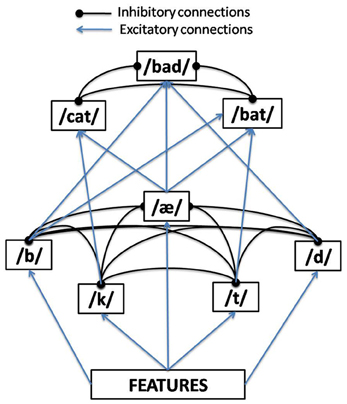
Figure 1. One time-slice of the TRACE model of spoken word recognition.
The details are more complex because of the way the model tackles the extremely difficult problem of recognizing series of phonemes or words that unfold over time, at a sub-phonemic grain. The solution implemented in TRACE is to take the conceptual network of Figure 1 and reduplicate every feature, phoneme, and word at successive timesteps. Time steps are meant to approximate 10 ms, and feature units are duplicated at every slice, while phonemes and words are duplicated every third slice. Thus, the phoneme layer can be visualized as a matrix with one row per phoneme and one column per time slice (i.e., a phonemes × slices matrix). However, units also have temporal extent—features for a given phoneme input extend over 11 time slices, ramping on and off in intensity. The same scheme is used at the lexical level, which can be visualized as a words × time slices matrix. Word lengths are not the simple product of constituent phoneme durations because phoneme centers are spaced six slices apart. This also gives TRACE a coarse analog to coarticulation; the features for successive phonemes overlap in time (but this is a weak analog, since feature patterns simply overlap and sometimes sum; but real coarticulation actually changes the realization of nearby and sometimes distant articulatory gestures). Each feature unit has forward connections to all phoneme units containing that feature that are aligned with it in time. Each phoneme unit has a forward connection to and a feedback connection from each word unit that “expects” that phoneme at that temporal location (so a /d/ unit at slice s has connections to /d/-initial words aligned near [at or just before or after] slice s, /d/-final words whose offsets are aligned at or adjacent to s, etc.). This more complex structure is shown in Figure 2.
Figure 2. The detailed structure of the TRACE model of spoken word recognition (adapted from McClelland and Elman, 1986).
The input to the model is transient; activation is applied to feature units “left-to-right” in time, as an analog of real speech input. Features that are activated then send activation forward. In IA networks, activation persists even after the removal of bottom–up input, as activation decays gradually rather than instantaneously. So as time progresses beyond the moment aligned with slice s, units aligned at slice s can continue to be active. A unit’s activation at a time step, t, is a weighted sum of its bottom–up input, its top–down input, and its own activation at time t-1, minus a decay constant. The crucial point in understanding TRACE is that time is represented in two different ways. First, stimulus time unfolds step-by-step, with bottom–up inputs for that step applied only in that step. Second, time-specific units at each level are aligned with a specific time step, t, but their activation can continue to wax and wane after the bottom–up stimulus has been applied at time t. This is because the model will only receive external input at time t, but activation will continue to flow among units aligned with time t as a function of bottom–up, top–down, and lateral connections within the model. This is what inspires the name “TRACE”: activation of a unit at time t is a constantly updating memory of what happened at time t modulated by lateral and top–down input.
In the original TRACE paper, McClelland and Elman presented results demonstrating how TRACE accounts for about 15 (depending on how one counts) crucial phenomena in human speech perception and spoken word recognition (see also Strauss et al., 2007 for a review). McClelland (1991) demonstrated how the addition of stochastic noise allowed TRACE to account properly for joint effects of context and stimulus (in response to a critique by Massaro, 1989). More recently, TRACE has been successfully applied to the fine-grained time-course of effects of phonological competition (Allopenna et al., 1998), word frequency (Dahan et al., 2001a), and subcateogorical (subphonemic) mismatches (Dahan et al., 2001b), using the visual world paradigm (Tanenhaus et al., 1995). In this paradigm, eye movements are tracked as participants follow spoken instructions to interact with real or computer-displayed arrays of objects (see Cooper, 1974, for an earlier, passive-task variant of the paradigm, the potential of which was not recognized at the time). While participants make only a few saccades per trial, by averaging over many trials, one can estimate the fine-grained time course of lexical activation and competition over time.
While some models have simulated aspects of visual world results (e.g., ShortlistB, Norris and McQueen, 2008), none has simulated the full set TRACE simulates, nor with comparable precision (although this assertion is based largely on absence of evidence—most models have not been applied to the full range of phenomena TRACE has; see Magnuson et al., 2012, for a review). While TRACE is not a learning model, its ability to account for such a variety of findings in a framework that allows one to test highly specific hypotheses about the general organization of spoken word recognition (for instance TRACE’s assumption of localist and separated levels of representations makes it easier to consider the impact of perturbing specific levels of organization, i.e., sublexical or lexical). However, while TRACE does an excellent job at fitting many phenomena, its translation of time to space via its time-specific reduplications of featural, phonemic and lexical units is notably inefficient (indeed, McClelland and Elman, 1986 noted it themselves; p. 77). In fact, as we shall describe in detail below, extending TRACE to a realistic phoneme inventory (40 instead of 14) and a realistic lexicon size (20,000 instead of 212 words) would require approximately 4 million units and 80 billion connections. To us, this begs a simple question: is it possible to create a model that preserves the many useful aspects of TRACE’s behavior and simplicity while avoiding the apparent inefficiency of reduplication of time-specific units at every level of the model? As we explain next, we take our inspiration from solutions proposed for achieving spatial invariance in visual word recognition in order to tackle the problem of temporal invariance in spoken word recognition.
1.1. Time and Trace: Man Bites God
Visual words have several advantages over spoken words as objects of perception. All their elements appear simultaneously, and they (normally) persist in time, allowing the perceiver to take as much time as she needs, even reinspecting a word when needed. In a series of words, spaces indicate word boundaries, making the idea of one-at-a-time word processing (rather than letter-by-letter sequential processing) possible. In speech, the components of words cannot occur simultaneously (with the exception of single-vowel words like “a”). Instead, the phonological forms of words must be recovered from the acoustic outcomes of a series of rapidly performed and overlapping (coarticulated) gymnastic feats of vocal articulators. A spoken word’s parts are transient, and cannot be reinspected except if they are held in quickly decaying echoic memory. In a series of words, articulation and the signal are continuous; there are no robust cues to word boundaries, meaning the perceiver must somehow simultaneously segment and recognize spoken words on the fly. Any processing model of spoken word recognition will need some way to code the temporal order of phonemes and words in the speech stream. There are four fundamental problems the model will have to grapple with.
First, there is the “temporal order problem,” which we might call the “dog or god” problem. If, for example, a model simply sent activation to word representations whenever any of their constituent phonemes were encountered without any concern for order, the sequences /dag/, /gad/, /agd/ (etc.) would equally and simultaneously activate representations of both dog and god. TRACE solves this by having temporal order built into lexical level units: a unit for dog is a template detector for the ordered pattern /d/-/a/-/g/, whereas a god unit is a template detector for /g/-/a/-/d/.
Second, there is the “multi-token independence problem,” or what we might call the “do/dude” or “dog eats dog” problem: the need to encode multiple instances of the same phoneme (as in words like dude, dad, bib, gig, dread, or Mississippi) or word (as in dog eats dog). That is, a model must be able to treat the two instances of /d/ in dude and the two instances of dog in dog eats dog as independent events. For example, if we tried having a simple model with just one unit representing /d/, the second /d/ in dude would just give us more evidence for /d/ (that is, more evidence for do), not evidence of a new event. The same would be true for dog eats dog; a single dog unit would just get more activated by the second instance without some way of treating the two tokens as independent events. TRACE achieves multi-token independence by brute force: it has literally independent detectors aligned at different time slices. If the first /d/ is centered at slice 6, the /a/ (both /a/ and /ae/ are represented by /a/ in TRACE) will be centered at slice 12 and the final /d/ will be centered at slice 18. The two /d/ events will activate completely different /d/ phoneme units. Thus, TRACE achieves multi-token independence (the ability to “recognize” two temporally distant tokens of the same type as independent) by having time-specific detectors.
Third is the “man bites dog” problem, which is the temporal order problem extended to multi-word sequences. The model must have some way to code the ordering of words; knowing that the words dog, man, and bites have occurred is insufficient; the model must be able to tell man bites dog from dog bites man. Putting these first three problems together, we might call them the “man bites god” problem—without order, lexical ambiguities will lead to later phrasal ambiguities. TRACE’s reduplicated units allow it to handle all three.
Finally, there is the “segmentation problem.” Even if we ignore the primary segmentation problem in real speech (the fact that phonemes overlap due to coarticulation) and make the common simplifying assumption that the input to spoken word recognition is a series of already-recognized phonemes, we need a way to segment words. It may seem that this problem should be logically prior to the “man bites dog” problem, but many theories and models of spoken word recognition propose that segmentation emerges from mechanisms that map phonemes to words. For example, in the Cohort model (Marslen-Wilson and Tyler, 1980), speech input in the form of phoneme sequences is mapped onto lexical representations (ordered phonological forms) phoneme-by-phoneme. When a sequence cannot continue to be mapped onto a single word, a word boundary is postulated (e.g., given the dog, a boundary would be postulated at /d/ because it could not be appended to the previous sequence and still form a word). TRACE was inspired largely by the Cohort model, but rather than explicitly seeking and representing word boundaries, segmentation is emergent: lateral inhibition among temporally-overlapping word units forces the model to settle on a series of transient, temporary “winners”—word units that dominate at different time slices in the “trace.”
Solving several problems at once is compelling, but the computational cost is high. Specifically, because TRACE relies on reduplication at every time slice of features, phonemes, and words, the number of units in the model will grow linearly as a function of the number of time slices, features, phonemes, and words. But because units in TRACE have inhibitory links to all overlapping units at the same level, the number of connections grows quadratically as units at any level increase. Scaling up the 14 phonemes in the original TRACE model to the approximately 40 phonemes in the English inventory would not in itself lead to an explosive increase in units or connections (see Appendix A). Moving from the original TRACE lexicon of just 212 words to a realistically-sized lexicon of 20,000 words, however, would. In fact, the original TRACE model, with 14 phonemes and 212 words would require 15,000 units and 45 million connections. Increasing the phoneme inventory would change the number of units to approximately 17,000 and the number of connections to 45.4 million. Increasing the lexicon to 20,000 words would result in 1.3 million units and 400 billion connections. How might we construct a more efficient model?
1.2. Visual and Spoken Word Recognition
There are several reasons to believe that visual and spoken word recognition could share more mechanisms than is usually appreciated. To be sure, very salient differences exist between the visual and auditory modalities. One signal has a temporal dimension, the other is spatially extended. The former travels sequentially (over time) through the cochlear nerve, the latter in parallel through the optic nerve. In addition, just as in spoken word recognition, researchers in the field of visual word recognition have to ponder an invariance problem. Although a unique fixation near the center of a word is usually enough for an adult to recognize it (Starr and Rayner, 2001), ultimately this fixation has only stochastic precision and will rarely bring the same stimulus twice at exactly the same place on the retina, resulting in dissimilar retinal patterns. A credible model of the visual word recognition system should find a way to overcome this disparity in a word’s many location exemplars, and to summon a unique lexical meaning and a unique phonology independently of wherever the visual stimulus actually fell on the retina.
1.3. String Kernels
In the machine learning literature, one computational technique that has been very successful at comparing sequences of symbols independently of their position goes under the name of string kernels (Hofmann et al., 2007). Symbols could be amino-acids, nucleotides, or letters in a webpage: in every case the gist of string kernels is to represent strings (such as “TIME”) as points in a high-dimensional space of symbol combinations (for instance as a vector where each component stands for a combination of two symbols, and only the components for “TI,” “TM,” “TE,” “IM,” “IE,” “ME” would be non-zero). It is known that this space is propitious to linear pattern separations and yet can capture the (domain-dependent) similarities between them. String kernels have also been very successful due to their computability: it is not always necessary to explicitly represent the structures in the space of symbol combinations in order to compute their similarity (the so-called “kernel trick,” which we will not use here).
It has been argued that string kernels provide a very good fit to several robust masked priming effects in visual word recognition, such as for instance letter transposition effects (the phenomenon that a letter transposition like trasnpose better primes the original word than a stimulus with letter replacements, such as tracmpose), and are thus likely involved at least in the early stages of visual word encoding (Hannagan and Grainger, 2012). To our knowledge, however, there have been no published investigations of string kernels in the domain of spoken word recognition. While the notion of an open biphone may at first blush sound implausible, keep in mind that the open bigram string kernel approach affords spatial invariance for visual word recognition. Might it also provide a basis for temporal invariance for spoken words?
2. Tisk, the Time Invariant String Kernel Model of Spoken Word Recognition: Materials and Methods
2.1. General Architecture and Dynamics
Our extension of the string kernel approach to spoken words is illustrated in Figure 3. It uses the same lexicon and basic activation dynamics as the TRACE model, but avoids a massive reduplication of units, as it replaces most time-specific units from TRACE with time-invariant units. It is comprised of four levels: inputs, phonemes, nphones (single phones and diphones) and words. Inputs consist of a bank of time-specific input units as in TRACE, through which a wave of transient activation travels. However, this input layer is deliberately very simplified compared to its TRACE analog. The input is like the Dandurand et al. (2010) input layer, though in our case, it is a time slice × phoneme matrix rather than a spatial slot × letter matrix. Thus, for this initial assay with the model, we are deferring an implementation like TRACE’s pseudo-spectral featural level and the details it affords (such as TRACE’s rough analog to coarticulation, where feature patterns are extended over time and overlap). With our localist phoneme inputs, at any time there is always at most one input unit active—inputs do not overlap in time, and do not code for phonetic similarity (that is, the inputs are orthogonal localist nodes). Note that the use of time-specific nodes at this level is a matter of computational convenience without theoretical commitment or consequence; these nodes provide a computationally expedient way to pass sequences of phonemic inputs to the model, and could conceivably be replaced by a single bank of input nodes (but this would require other additions to the model to allow inputs to be “scheduled” over time). As in the TRACE model, one can construe these input nodes as roughly analogous to echoic memory or a phonological buffer. As we shall see, these simplifications do not prevent the model from behaving remarkably similarly to TRACE.
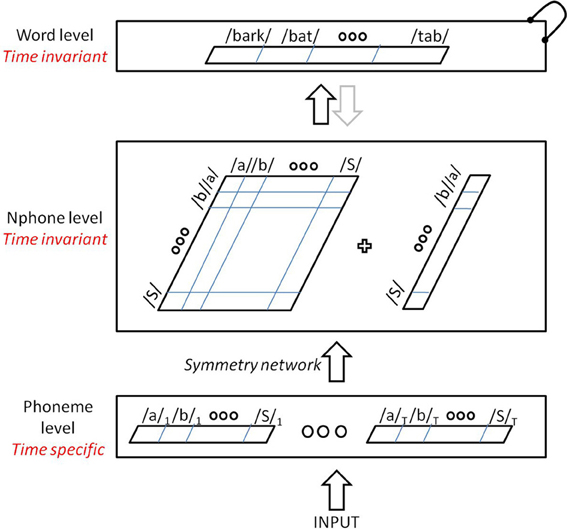
Figure 3. The TISK model—a time-invariant architecture for spoken word recognition.
For our initial simulations, the model is restricted to ten slices (the minimum number needed for single-word recognition given the original TRACE lexicon), each with 14 time-specific phoneme units (one for each of the 14 TRACE phonemes). The input phoneme units feed up to an nphone level with one unit for every phoneme and for every ordered pairing of phonemes. The nphone units are time-invariant; there is only one /d/ unit at that level and only one /da/ diphone unit. Finally, nphone units feed forward to time-invariant (one-per-word) lexical units.
A critical step in the model is the transition between the time-specific phoneme input level and the time-invariant nphone level. This is achieved via entirely feedforward connections, the weights of which are set following certain symmetries that we will describe shortly. The nphone level implements a string kernel and consists of 196 + 14 units, one for each possible diphone and phoneme given the TRACE inventory of 14 phonemes. Units at this level can compete with one another via lateral inhibition, and send activation forward to the time invariant word level through excitatory connections, whose weights were normalized by the number of nphones of the destination word. The word level consists of 212 units (the original TRACE lexicon), with lateral inhibitory connections only between those words that share at least one phoneme at the level below. For this preliminary investigation, feedback connections from words to nphones were not included.
Units in the model are leaky integrators: at each cycle t, the activation Ai of unit i will depend on the net input it receives and on its previous activation, scaled down by a decay term, as described in Equation (1):
where the net input of unit i at time t is given by:
Python code for the model is available upon request to the first author, and a list of parameters is provided below as supplemental data. In the next section, we describe in detail the connections between time-specific phonemes and time-invariant nphones.
2.2. From Time-Specific to Time-Invariant Units: A Symmetry Network for Phonological String Kernels
We now describe the transition phase between time-specific phonemes and time-invariant nphones in the TISK model. It is clear that unconstrained (that is, unordered) “open diphone” connectivity would be problematic for spoken words; for example, if dog and god activated exactly the same diphones (/da/, /dg/, /ag/, /ga/, /gd/, /ad/), the system would be unable to tell the two words apart. The challenge is to activate the correct diphone /da/, but not /ad/, upon presentation of a sequence of phonemes like [/d/t, /a/t + 1], that is, phoneme /d/ at time t and phoneme /a/ subsequently. Thus, the goal is to preserve activation of non-adjacent phonemes as in an open diphone scheme (for reasons explained below) with the constraint that only observed diphone sequences are activated—that is, dog should still activate a /dg/ diphone (as well as /da/ and /ag/) because those phonemes have been encountered in that sequence, but not /gd/, while god should activate /gd/ but not /dg/. This would provide a basis for differentiating words based on sequential ordering without using time-specific units “all the way up” through the hierarchy of the model.
The issue of selectivity (here, between “anadromes”: diphones with the same phonemes in different order) vs. invariance (here, to position-in-time) has long been identified in the fields of visual recognition and computer vision, and has recently received attention in a series of articles investigating invariant visual word recognition (Dandurand et al., 2010, 2013; Hannagan et al., 2011).
Directly relevant to this article, Dandurand et al. (2013) trained a simple perceptron network (that is, an input layer directly connected to an output layer, with weights trained using the delta rule) to map location-specific strings of letters to location-invariant words. To their surprise, not only did this simplistic setup succeed in recognizing more than 5000 words, a fair fraction of which were anagrams, it also produced strong transposition effects. By introducing spatial variability—the “i” in science could occur in many different absolute positions rather than just one—tolerance for slight misordering in relative position emerged. When Dandurand et al. (2013) investigated how the network could possibly succeed on this task in the absence of hidden unit representations, they observed that during the course of learning, the “Delta learning rule” had found an elegant and effective way to keep track of letter order by correlating connection strengths with the location of the unit. More precisely, the connections coming from all “e” units and arriving at word live had their weights increasing with the position, whereas the connections from the same units to the word evil had their weights decreasing with position. In this way, connection weights became a proxy for the likelihood of a word given all letters at all positions. This simple scheme enabled the network to distinguish between anagrams like evil and live. We describe next how this solution found by the delta rule can be adapted to map time-specific phonemes to time-invariant diphones or single phonemes.
The network in Figure 4 has two symmetries: firstly, weights are invariant to changes in input phoneme identity at any given time. This is manifest in Figure 4 by the symmetry along the medial vertical axis: for any t, at and bt can exchange their weights. Secondly, weights are invariant to changes in input phonemes identity across opposite times (in Figure 4), a central symmetry with center midway through the banks of input phonemes: for any t ≤ T, at and bT − t are identical, and so are bt and aT − t. Although the first symmetry concerns both excitatory (arrows) and gating connections (crosses, which will be shortly explained), the second symmetry concerns only excitatory connections.
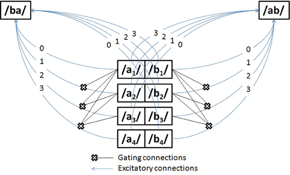
Figure 4. A symmetry network for time-invariant nphone recognition that can distinguish anadromes. The units in the center of the diagram (e.g., /a/1) represent time-specific input nodes for phonemes /a/ and /b/ at time steps 1–4. The /ba/ and /ab/ nodes represent time-invariant diphone units.
What is the point of these symmetries? Consider a network where the weights have been set up as in Figure 4. Then at all possible times t, presenting the input sequence [/a/t, /b/t + 1] by clamping the appropriate units to 1 will always result in a constant net input for /ab/, here a net input of 4, and it will always result in a smaller constant net input to /ba/, here a net input of 2. A common activation threshold for every diphone unit can then be set anywhere between these two net inputs (for instance, a threshold of 3), that will ensure that upon perceiving the sequence [/a/t, /b/t + 1] the network will always recognize /ab/ and not /ba/. The same trick applies for the complementary input sequence [/b/t, /a/t + 1], by setting the weights from these phoneme units to the transposed diphone /ba/ in exactly the opposite pattern. A subtlety, however, is that in order to prevent sequences with repeated phonemes like [/b/1, /a/2, /b/3] from activating large sets of irrelevant nphones like /br/ or /bi/, it is necessary to introduce gating connections (cross-ended connections in Figure 4), whereby upon being activated, unit /b/1 will disable the connection between all future /b/t >1 and all diphones /*b/ (where “*” stands for any phoneme but b).
The use of gating connections is costly, as the number of connections needed is proportional to the square of the number of time slices, but less naïve gating mechanisms exist with explicit gating units that would be functionally equivalent at a much smaller cost (linear with increasing numbers of time slices). More generally, other mappings between time-specific phonemes and time-invariant n-phones are possible. However, our approach is cast within the theory of symmetry networks (Shawe-Taylor, 1993), which ensures that several mathematical tools are available to carry out further analysis. The particular symmetry network introduced here arguably also has a head-start in learnability, given that it builds on a solution found by the delta rule. Specifically, in a perceptron trained to recognize visual words (Dandurand et al., 2013), the Delta rule found the “central symmetry through time” visible in Figure 4. We do not know if pressure to represent temporal sequences would allow the model to discover the “axial” symmetry and necessity for gating connections, but this is a question we reserve for future research. We note that some studies have reported the emergence of symmetry networks in more general settings than the delta rule and word recognition, that is, under unsupervised learning algorithms and generic visual inputs (Webber, 2000). Perhaps the best argument for this architecture is that it is reliable, and allows for the activation of the kind of “string kernels” recently described by Hannagan and Grainger (2012), at a computational cost that can be regarded as an upper-bound and yet is not prohibitive.
3. Results
3.1. Performance on Single Word Recognition
We begin with a comparison of TISK and TRACE in terms of the recognition time of each word in the original 212-word TRACE lexicon. If TISK performs like TRACE, there should be a robust correlation between the recognition time for any particular word in the two models. We operationalized spoken word recognition in three different ways: an absolute activation threshold (Rabs), a relative activation threshold (Rrel) and a time-dependent criterion (Rtim). The first criterion states that a word is recognized if its activation reaches an absolute threshold, common to all words. In the second criterion, recognition is granted whenever a word’s activation exceeds that of all other words by a threshold (0.05 in the simulations). Finally the time-dependent criterion defines recognition as a word’s activation exceeding that of all other words for a certain number of cycles (10 cycles in the simulations).
Spoken word recognition accuracy for TRACE is consistently greater than that for TISK in these simulations, although both models obtain high performance under all criteria. TRACE exhibits close to perfect recognition with the three criteria (Tabs = 97%, Trel = 99%, Ttim = 99%). TISK on the other hand operates less well under an absolute criterion, but recognition is improved using a relative threshold, and it rises to TRACE-like level with a time-dependent threshold (Tabs = 88%, Trel = 95%, Ttim = 98%). Also, mean recognition cycles are similar for TRACE (Tabs = 38 cycles, Trel = 32 cycles, Ttim = 40 cycles) and for TISK (Tabs = 45 cycles, Trel = 38 cycles, Ttim = 40 cycles). At the level of individual items, performance is very similar for the two models, as revealed by high correlations between recognition times (for correctly recognized items) under all three recognition definitions (r for each definition: Tabs = 0.68, Trel = 0.83, Ttim = 0.88). Figure 5 illustrates the correlation between response times in the case of Ttim. In the rest of this article we will use the time-dependent criterion Ttim, as the one with which models achieved both the best performance and the most similar performance.
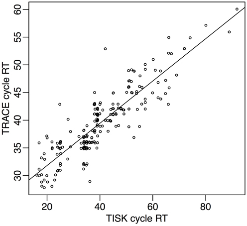
Figure 5. Response times in TISK (x-axis) and TRACE (y-axis) for all 212 words in the lexicon, when a time threshold is used for recognition.
It is also instructive to consider the two words on which TISK failed, /triti/ (treaty) and /st^did/ (studied). Indeed the model confused these words with their respective embedded cohort competitors /trit/ (treat) and /st^di/ (study). For the model these are the most confusable pairs of words in the lexicon, because in each case almost exactly the same set of nphones is activated for the target and the cohort competitor, except for one or two n-phones (the only additional diphone for treaty compared to treat is /ii/; studied activates two additional diphones compared to study: /dd/ and /id/). It is certainly possible to fine-tune TISK so as to overcome this issue. Note also that TISK recognizes correctly the vast majority of words containing embeddings, including word-onset embeddings.
But these particular failures are perhaps more valuable in that they point to the type of learning algorithm that could be used in the future, in TISK as in TRACE, to find the connection weights in a more principled manner. Namely, they strongly suggest that a learning algorithm should attribute more weight to these connections that are the most diagnostic given the lexicon (e.g., connection /ii/ to /triti/).
3.2. Time Course of Lexical Competitors
As previously observed, what is impressive about the TRACE model is less its ability to recognize 212 English words than the way it does so, which captures and explains very detailed aspects of lexical competition in human spoken word recognition. Consider the so-called “Visual World Paradigm” (Tanenhaus et al., 1995), in which subjects’ eye movements are tracked as they follow verbal instructions to manipulate items in a visual display. When the items include objects with similar sounding names (e.g., so-called “cohort” items with the same word onset, such as beaker and beetle, or rhymes, such as beaker and speaker) as well as unrelated items to provide a baseline, eye movements provide an estimate of activation of concepts in memory over time. That is, the proportion of fixations to each item over time maps directly onto phonetic similarity, with early rises in fixation proportions to targets and cohorts and later, lower fixation proportions to rhymes (that are still fixated robustly more than unrelated items; Allopenna et al., 1998). Allopenna et al. also conducted TRACE simulations with items analogous to those they used with human subjects, and found that TRACE accounted for more than 80% of the variance in the over-time fixation proportions.
In order to assess how TISK compares to TRACE in this respect, we subjected the model to simulations analogous to those used by Allopenna et al. (1998). However, rather than limiting the simulations to the small subset of the TRACE lexicon used by Allopenna et al., we actually conducted one simulation for every (correctly recognized) word in the TRACE lexicon with both TRACE and TISK. We then calculated average target activations over time, as well as the over-time average activation of all cohorts of any particular word (words overlapping in the first two phonemes), any rhymes, and words that embed in the target (e.g., for beaker, these would include bee and beak, whereas for speaker, these would be speak, pea, peek). Rather than selecting a single word to pair with each word as its unrelated baseline, we simply took the mean of all words (including the target and other competitors); because most words are not activated by any given input, this hovers near resting activation levels (−0.2 for TRACE, 0 for TISK). The results are shown in Figure 6.
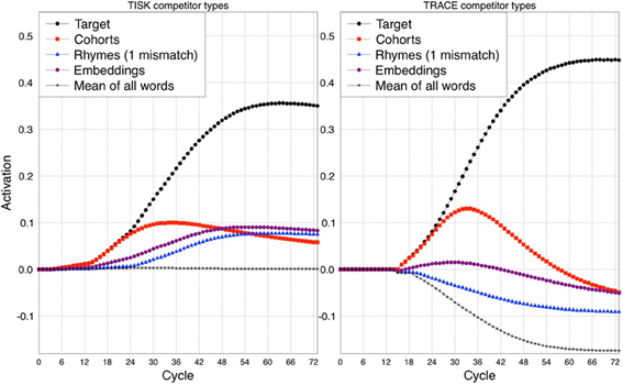
Figure 6. Comparison between TISK (left panel) and TRACE (right panel) on the average time-course of activation for different competitors of a target word. Cohort: initial phonemes shared with the target. Rhymes (1 mismatch): all phonemes except the first shared with the target. Embeddings: words that embed in the target. The average time course for all words (Mean of all words) is presented as a baseline.
Readers familiar with the Allopenna et al. article will notice some differences in our TRACE simulation results compared to theirs. First, we have activations below zero, while they did not. This is because Allopenna et al. followed the standard practice of treating negative activations as zero. Second, our rhyme activations remain below zero, even though they are robustly higher than those of the mean activation baseline. Having robustly positive rhyme activations in TRACE requires the use of a carrier phrase like the one used by Allopenna et al. (or a transformation to make all activations above resting level positive); without this, because there is strong bottom–up priority in TRACE, cohorts will be so strongly activated that rhyme activation will be difficult to detect. However, what really matters for our purposes is the relative activations of each competitor type, which are clearly consistent between the two models.
3.3. Lexical Factors Influencing Recognition
Let’s return to item level recognition times. We can probe the models more deeply by investigating how recognition times vary in each model with respect to the lexical dimensions that have attracted the most attention in the spoken word recognition literature. Figure 7 presents the correlation between recognition cycles and six standard lexical variables: the length of the target (Length), how many words it embeds in (Embeddings), how many words embed in it (Embedded), how many deletion/addition/subsitution neighbors it has (Neighbors), the number of words with which it shares 2 initial phonemes (Cohorts), and the number of words that overlap with it when its first phoneme is removed (Rhymes).
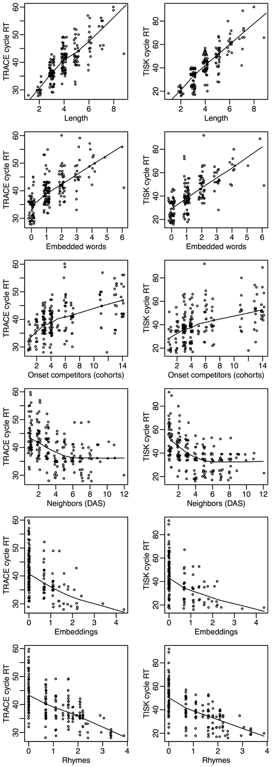
Figure 7. An overview of how recognition cycles correlate with other lexical variables in TRACE (left column) and in TISK (right column). Length: target length. Embedded words: number of words that embed in the target. Onset competitors (Cohorts): number of words that share two initial phonemes with the target. Neighbors (DAS): count of deletion/addition/subsitution neighbors of the target. Embeddings: logarithm of the number of words the target embeds in. Rhymes: logarithm of the number of words that overlap with the target with first phoneme removed.
Figure 7 shows that among the six lexical dimensions considered, three are inhibitory dimensions (Length, Embedded words and Cohorts) and three are clearly facilitatory dimensions (Neighbors, Embeddings, and Rhymes). Crucially, precisely the same relationships are seen for both models, with an agreement that is not only qualitative but also quantitative.
Facilitatory variables are perhaps the most surprising, as neighborhood has long been construed as an inhibitory variable for spoken word recognition. Although the precise details are not relevant for this initial presentation of TISK, further inspection of these neighborhood effects reveals that there is an interaction of neighborhood with word length; for longer words, neighbors begin to have a facilitative effect. The crucial point is that one can see that TRACE and TISK behave in remarkably similar ways—and both make intriguing, even counter-intuitive, but testable predictions.
3.4. Computational Resources
We will end this comparison with an assessment of the resources needed in both models. Table 1 shows the number of connections and units in TRACE and TISK, as calculated in Appendix C. The figures for TRACE are obtained by considering the number of units required per slice in the model (starting from the phoneme level, for a fair comparison with TISK which doesn’t use a featural level): 14 phonemes, and, in the basic TRACE lexicon, 212 words, for 226 units. Now assuming an average of 3 phonemes per word, and allowing for connections between units at adjacent time slices, TRACE needs approximately 225,000 connections per time slice. If we make the trace 200 time slices long (which assuming 10 ms per slice would amount to 2 s, the duration of echoic memory), we need approximately 15,000 units and 45 million connections. Increasing the lexicon to a more realistic size of 20,000 words and the phoneme inventory to 40, these figures reach approximately 1.3 million units and 400 billion connections.
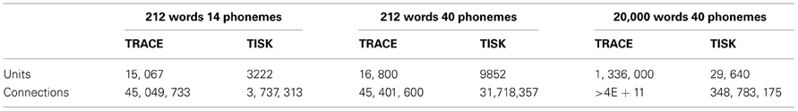
Table 1. Estimates of the number of units and connections required in TRACE and TISK for 212 or 20,000 words, 14 or 40 phonemes, an average of four phonemes per word, and assuming 2 s of input stream.
Next let us consider the situation in TISK. With a 2 s layer of time-specific input units (again, corresponding to the approximate limit of echoic memory), 14 phonemes and 212 words as in TRACE, TISK requires 3.2 thousand units and 3.7 million connections. This represents a 5-fold improvement over TRACE for units, and a 15-fold improvement for connections. With 20,000 words and 40 phonemes, TISK would require approximately 29,000 units (TRACE requires 45 times more) and 350 million connections (TRACE requires 1.1 thousand times more).
Figure 8 presents an overview of the number of connections as a function of trace duration (number of time slices) and lexicon size in TISK and in TRACE. The most striking feature already apparent in Table 1 is that TRACE shows an increase in connections which dwarfs the increase in TISK. But Figure 8 also shows that in TRACE this increase is quadratic in lexicon size and steeply linear in time slices, while connection cost in TISK looks linear in both variables with very small slopes. While Appendix B demonstrates that both functions are actually quadratic in the number of words (due to lateral inhibition at the lexical level in both models), there is still a qualitative difference in that the quadratic explosion due to the word level is not multiplied by the number of time slices in TISK, like it is in TRACE—decoupling trace duration and lexicon size was, after all, the whole point of this modeling exercise.
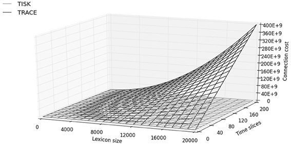
Figure 8. Number of connections (y-axis, “connection cost”) as a function of time slices and lexical size in TISK (gray surface) and TRACE (black surface).
What is the significance of this computational economy for spoken word recognition? We would argue that it makes it easier to examine the behavior of the model at large scales. The 400 billion connections required in TRACE currently discourage any direct implementation with a realistic lexicon. However, word recognition behavior in IA models like TRACE and TISK is exquisitely sensitive to the nature of lexical competition. One should therefore not be content with effects obtained using an artificial sample of 200 words but should aim at running the model on the most realistic lexicon possible.
Depending on the precise linking assumptions one is willing to make between units and connections on the one hand, and actual neurons and synapses on the other hand (see, for instance, de Kamps and van der Velde, 2001 for a well-motivated attempt), one may or may not find that for some large but still reasonable lexicon size the connection cost in TRACE becomes larger than the sum total of all available synapses in the brain, whereas Figure 8 and Appendix B suggest that the cost in TISK would be orders of magnitude smaller and may barely make a dent in the synaptic budget.
But even leaving aside this possibility, the notion that wiring cost should come into consideration when modeling cognitive systems appears to be rather safe. Firing neurons and maintaining operational synapses has a high metabolic cost, and the pressure to perform such a ubiquitous task as spoken word recognition would seem to demand an implementation that balances cost and efficiency in the best possible way. Although the connections in TRACE or TISK are meant to be functional rather than biological, metabolic costs at the biological level constrain connectivity at the functional level: numerous functional networks as derived from human brain imaging achieve economical trade-offs between wiring cost and topological (connectivity) efficiency (Bullmore and Sporns, 2012). Recent investigations with artificial neural networks have also shown that minimizing the number of connections can improve performance by favoring the emergence of separate levels of representations (Clune et al., 2013).
4. Discussion
4.1. Spoken and Visual Word Recognition: A Bridge Between Orthography and Phonology
In 1981, McClelland and Rumelhart presented an interactive-activation model of visual word recognition that was to be a major inspiration for the TRACE model of spoken word recognition (McClelland and Elman, 1986) and an inspiration for future generations of reading researchers. Most important is that in Figure 1 of their article, McClelland and Rumelhart sketched an overall architecture for visual and auditory word perception, describing interconnections between the two in the form of reciprocal letter-phoneme connections. This architecture clearly predicts that visual word recognition should be influenced on-line by phonological knowledge and spoken word recognition should be influenced by orthographic knowledge. Support for these predictions has since been provided by a host of empirical investigations (see Grainger and Ziegler, 2008 for a review). Strangely enough, however, attempts to implement such a bi-modal architecture have been few and far between. Research on visual word recognition has come the closest to achieving this, with the development of computational models that include phonological representations (Seidenberg and McClelland, 1989; Plaut et al., 1996; Coltheart et al., 2001; Perry et al., 2007).
With respect to spoken word recognition, however, to our knowledge no computational model includes orthographic representations, and although our TISK model of spoken word recognition is not an improvement in this respect, it was nevertheless designed with the constraint of eventually including such representations in mind. As such, TISK not only provides an answer to McClelland and Elman’s question of how to avoid duplication in TRACE, but also picks up on McClelland and Rumelhart’s challenge to develop a truly bimodal model of word recognition. One model has been developed along the lines initially suggested by McClelland and Elman (1986)—this is the bimodal interactive-activation model (Grainger et al., 2003; Grainger and Holcomb, 2009), recently implemented by Diependaele et al. (2010). Future extensions of this work require compatibility in the way sublexical form information is represented for print and for speech. The present work applying string kernels to spoken word recognition, along with our prior work applying string kernels to visual word recognition (Hannagan and Grainger, 2012), suggest that this particular method of representing word-centered positional information provides a promising avenue to follow. Indeed, string kernels provide a means to represent order information independently of whether the underlying dimension is spatial or temporal, hence achieving spatial invariance for visual words and temporal invariance for spoken words.
4.2. Testing for Temporal Invariance in Spoken Word Recognition
Researchers interested in the neural representations for visual words are blessed with the Visual Word Form Area, a well-defined region in the brain that sits at the top of the ventral visual stream, and is demonstratively the locus of our ability to encode letter order in words or in legal non-words (Cohen et al., 2000; Gaillard et al., 2006) but is not selectively activated for spoken words. Until recently, the common view was that by the mere virtue of its situation in the brain, if not by its purported hierarchical architecture with increasingly large receptive fields, the VWFA was bound to achieve complete location invariance for word stimuli. However, recent fMRI studies show that, and computational modeling explains why, a significant degree of sensitivity to location is present in the VWFA (Rauschecker et al., 2012). A trained, functional model of location invariance for visual words explains why this can be so (Hannagan and Grainger, in press). In this model the conflicting requirements for location invariant and selectivity conspire with limited resources, and force the model to develop in a symmetry network with broken location symmetry on its weights (Hannagan et al., 2011). This in turn produces “semi-location invariant” distributed activity patterns, which are more sensitive to location for more confusable words (Hannagan and Grainger, in press). Thus brain studies have already been highly informative and have helped constrain our thinking on location invariance in visual words.
But attempts to proceed in the same way for the auditory modality quickly run into at least two brick walls. The first is that a clear homologue of the VWFA for spoken words has remained elusive. This might be because the speech signal varies in more dimensions than the visual signal corresponding to a visual object; a VWFA homologue for speech might need to provide invariance not just in temporal alignment, but also across variation in rate, speaker characteristics, etc. However, one study points to the left superior temporal sulcus as a good candidate for an Auditory Word Form Area (AWFA) on the grounds that this region only responded for auditory words and showed repetition suppression when the same word was spoken twice (Cohen et al., 2004), and there have been reports of invariance for temporal alignment or speaker characteristics and/or multidimensional sensitivity in the superior (Salvata et al., 2012) and medial (Chandrasekaran et al., 2011) temporal gyri. The second issue is that paradigms for testing temporal invariance are less easily designed than those which test location invariance in the visual case. Speculating from Rauschecker et al. (2012), however, we can propose a task that tests for the presence of time-specific word representations, in which subjects would be presented with a sequence of meaningless sounds where one spoken word would be embedded. By manipulating the position of this word in the sequence, one could then test whether a “blind” classifier could be trained to discriminate by their positions-in-time the different fMRI activation patterns evoked in the superior temporal sulcus. Because this decoding procedure can be applied to signals recorded from several disconnected regions of interest, this procedure would be agnostic to the existence of a well-circumscribed AWFA. TRACE and TISK both predict that the classifier should succeed with fMRI patterns evoked early on in the processing stream, i.e., at the time-specific phoneme level, but only TISK predicts that time-invariant representations should be found downstream, for lexical representations. Although the necessity for testing the existence of time-specific units is obvious in the light of the TISK model, we would argue that this has long been an urgent experimental question to ask. TRACE has been the most successful model of spoken word recognition for almost three decades now, and therefore it might be worth taking seriously the most striking hypothesis it makes of the existence of time-specific units, an hypothesis which even TISK does not succeed in completely avoiding at the phoneme level.
4.3. Previous Models and Alternative Approaches to Temporal Order
We claimed previously that TRACE has the greatest breadth and depth of any extant model of spoken word recognition. Of course, there are models whose proponents argue that they have solved key problems in spoken word recognition without using TRACE’s inefficient time-specific reduplication strategy. We will review a few key examples, and consider how they compare with TRACE and TISK.
Norris (1994), Norris et al. (2000), and Norris and McQueen (2008) introduced Shortlist, Merge, and Shortlist B, the first two being IA network models and the latter a Bayesian model of spoken word recognition. All three models share basic assumptions, and we refer to them collectively as “the Shortlist models.” Contrary to TRACE, the Shortlist models are entirely feedforward. They also make a critical distinction between words and tokens, the latter being time-specific entities that instantiate the former, time-invariant lexical templates. The reduplication of the lexical level that afflicts TRACE is avoided in these models by assuming that only a “short list” of tokens is created and wired on-the-fly into a “lattice” of lexical hypotheses. These models have a sizable lexicon (even a realistic 20,000 word lexicon in the case of Shortlist B), and although they have not been applied to the full range of phenomena that TRACE has, they have successfully simulated phenomena such as frequency and neighborhood effects. Unfortunately, because no computational mechanism is described that would explain how the on-the-fly generation and wiring of tokens could be achieved, the account of spoken word recognition provided by Shortlist is still essentially promissory.
Other approaches to temporal order use fundamentally different solutions than TRACE’s reduplication of time-specific units. Elman’s (1990) simple recurrent network (SRN) may be foremost among these in the reader’s mind. The SRN adds a simple innovation to a standard feedforward, backpropagation-trained two-layer network: a set of context units that provide an exact copy of the hidden units at time step t-1 as part of the input at time t, with fully connected, trainable weights from context to hidden units. This feedback mechanism allows the network to learn to retain (partial) information about its own state at preceding time steps, and provides a powerful means for sequence learning. However, while SRNs have been applied to speech perception and spoken word recognition (most notably in the Distributed Cohort Model: Gaskell and Marslen-Wilson, 1997, but for other examples see Norris 1990, and Magnuson et al. 2000, 2003), so far as we are aware, no one has investigated whether SRNs can account for the depth and breadth of phenomena that TRACE does (though SRNs provide a possible developmental mechanism since they are learning models, and the Distributed Cohort Model has been applied to semantic phenomena beyond the scope of TRACE).
Another approach is the cARTWORD model of Grossberg and Kazerounian (2011), where activity gradients specific to particular sequences can differentiate orderings of the same elements (e.g., ABC vs. ACB, BAC, etc.). However, this mechanism cannot represent sequences with repeated elements (for example, it cannot distinguish ABCB from ABC, as the second B would simply provide further support for B rather than a second B event), which makes it incapable of representing nearly one third of English lemmas. Furthermore, it is premature to compare this approach to models like TRACE, since it has been applied to a single phenomenon (phoneme restoration) with just a few abstract input nodes and just a few lexical items; thus, we simply do not know whether it would scale to handle realistic acoustic-phonetic representations and large lexicons, let alone the broad set of phenomena TRACE accounts for (see Magnuson submitted, for detailed arguments and simulations showing that the supposed failures of TRACE to account for phoneme restoration phenomena reported by Grossberg and Kazerounian 2011, were the result of flawed simulations, not a problem with TRACE). Note that a similar activity gradient approach in visual word recognition (Davis, 2010) has also been attempted, with similar limitations.
4.4. The Utility of Interactive Activation Models
Because spoken word recognition is a slowly acquired skill in humans, any model of it should eventually strive to incorporate some kind of learning algorithm that explains how the representations necessary to solve the task have matured. Unlike SRNs though, models such as TRACE and TISK do not comply to this requirement. On the other hand and until proven the contrary TRACE vastly outperforms SRNs in explanatory power while having the advantage of being more transparent. We would argue that IA models and learning models like SRNs should be construed as complementary approaches to spoken word recognition. Imagine SRNs were demonstrated to account for similar depth and breadth as TRACE. We would still be left with the puzzle of how they do so. Unpacking the complex composites of cooperative and competitive wiring patterns that would develop would be no mean feat. This is where we find interactive activation models like TRACE and TISK especially useful. The IA framework allows one to construct models with levels of organization (the representational levels) with inter- and intralevel interaction governed by discrete parameters. This allows one to generate hypotheses about which aspects of the model are crucial for understanding some phenomenon (e.g., by investigating which model parameters most strongly generate a key behavior), or about which level of organization may be perturbed in a particular language disorder (Perry et al., 2010; Magnuson et al., 2011). One modeling approach that is likely to be productive is to use simpler frameworks like IA models to generate hypotheses about key model components in some behavior or disorder, and then to seek ways that such behaviors or disruptions might emerge in a more complex model, such as an SRN or another type of attractor network (cf. Magnuson et al., 2012). Similarly, TISK provides a testbed for investigating whether a string kernel scheme is a robust basis for spoken word recognition. For example, the success of string kernel representations in TISK might suggest that we should investigate whether the complex wiring SRNs learn approximates string kernels.
4.5. Relationship Between Trace and Tisk
One might be surprised that TISK and TRACE display such similar behavior despite the lack of feedback in the former and its presence in the latter. Feedback in models of spoken word recognition is a controversial topic (McClelland et al., 2006; McQueen et al., 2006; Mirman et al., 2006a), which we do not address here; our aim is to see whether a model with a radically simpler computational architecture compared to TRACE can (begin to) account for a similar range of phenomena in spoken word recognition. However, this resemblance despite feedback is less surprising than it may seem. Indeed, it has been known for several years that the feedback contribution to word recognition in TRACE is limited given noise-free input (Frauenfelder and Peeters, 1998): simulations show that feedback makes the model more efficient and robust against noise (Magnuson et al., 2005). It also provides an implicit sensitivity to phonotactics—the more often a phoneme or n-phone occurs in lexical items, the more feedback it potentially receives—and it is the mechanism by which top–down lexical effects on phoneme decisions are explained in TRACE. None of these effects were considered in this article, which focused on core word recognition abilities and lexical competition effects. We acknowledge that without feedback, TISK will not be able to simulate many top–down phenomena readily simulated in TRACE. Future research with TISK will explore the impact of feedback connections.
4.6. Limitations and Next Steps
The aim of this study was to improve on one particularly expensive aspect of the TRACE model without drastically affecting its lexical dynamics, or diminishing its explanatory power. We have demonstrated that a radically different approach to sequence representation, based on string kernels, provides a plausible basis for modeling spoken word recognition. However, our current model has several obvious limitations.
First, to apply TISK to the full range of phenomena to which TRACE has been applied will require changes, for example, in the input representations for TISK. As we mentioned above, we used single-point inputs for TISK rather than the on- and off-ramping, over-time inputs in TRACE that also give the model a coarse analog to coarticulation. An input at least this grain will be required to apply TISK to, for example, subcategorical mismatch experiments that TRACE accounts for (Dahan et al., 2001b).
Second, TISK’s levels and representations are stipulated rather than emergent. Our next step will be to examine whether codes resembling string kernels emerge when intra-level weights are learned rather than stipulated. What learning algorithm could find the set of weight values under which TISK and TRACE have been shown to achieve close to perfect recognition? Is there more than one such set, and do they make different predictions from the existing fine-tuned solutions? There are a few results that suggest the way forward. For instance, there are demonstrations that Hebbian learning applied at the lexical level in TRACE can help explain short term phenomena in spoken word recognition (Mirman et al., 2006b). If Hebbian learning is indeed active on short scales, there are no reasons to doubt that it will be involved on longer time-scales, slowly shaping the landscape of inhibition between words, which forms the basis for much of the behaviors explored in this article.
Third, a problem shared by all models of word recognition is that it is not clear how to scale from a model of word recognition to higher levels, e.g., to a model of sentence comprehension. Because TISK’s word level is time-invariant, there is no obvious way to generate ngrams at the word level. However, TISK and TRACE, like other models capable of activating a series of words over time given unparsed input (i.e., word sequences without word boundary markers) should be linkable to parsing approaches like “supertagging” (Bangalore and Joshi, 1999; Kim et al., 2002) or the self-organizing parser (SOPARSE) approach of Tabor et al. (e.g., Tabor and Hutchins, 2004). Note that a common intuition is that SRNs provide a natural way of handling sequential inputs from acoustics to phonemes to words. However, it is not clear that this translates into a comprehensive model of the entire speech chain. It is not apparent that you could have a single recurrent network that takes in acoustics and somehow achieves syntactic parsing (let alone message understanding) while producing human-like behavior at phonetic, phonological, lexical levels. These are non-trivial and unsolved problems, and despite the intuitive appeal of recurrent networks, remain unanswered by any extant model.
Finally, it is notable that we have not implemented feedback yet in TISK. This renders TISK incapable of accounting for top–down lexical effects on phoneme decisions. However, as Frauenfelder and Peeters (1998) and Magnuson et al. (2005) have demonstrated, feedback plays little role in recognition given clear inputs. When noise is added to a model like TRACE, feedback preserves speed and accuracy dramatically compared to a model without feedback. While feedback also provides a mechanistic basis for understanding top–down effects, it is also remarkable that at least one effect attributed to feedback in TRACE (rhyme effects; Allopenna et al., 1998) emerges in TISK without feedback. This suggests that in fact examining which, if any (other), putatively top–down effects emerge without feedback in TISK will be a useful enterprize. Given, however, the remarkable fidelity to TRACE that TISK demonstrates over a broad swath of phenomena, it is clear that feedback need not be included in this first assay with TISK.
5. Conclusion
Twenty-seven years after Elman and McClelland introduced the TRACE model, we have endeavored to answer the question of how to dispense with time-duplication, and have presented an alternative that preserves TRACE-like performance on spoken word recognition while using orders of magnitude less computational resources. Perhaps more importantly, the particular structures and mechanisms that achieve time-invariance in TISK construct new and intriguing bridges between visual and spoken word recognition.
Funding
Thomas Hannagan and Jonathan Grainger were supported by ERC research grant 230313.
Conflict of Interest Statement
The authors declare that the research was conducted in the absence of any commercial or financial relationships that could be construed as a potential conflict of interest.
Acknowledgments
We thank Emily Myers, Lori Holt, and David Gow Jr., for stimulating discussions.
References
Allopenna, P. D., Magnuson, J. S., and Tanenhaus, M. K. (1998). Tracking the time course of spoken word recognition: evidence for continuous mapping models. J. Mem. Lang. 38, 419–439. doi: 10.1006/jmla.1997.2558
CrossRef Full Text
Bangalore, S., and Joshi, A. (1999). Supertagging: an approach to almost parsing. Comput. Linguisti. 25, 238–265.
Bowers, J. S., Damian, M. F. E., and Davis, C. J. (2006). A fundamental limitation of the conjunctive codes learned in PDP models of cognition: comments on Botvinick and Plaut. Psychol. Rev. 116, 986–997. doi: 10.1037/a0017097
Pubmed Abstract | Pubmed Full Text | CrossRef Full Text
Chandrasekaran, B., Chan, A. H. D., and Wong, P. C. M. (2011). Neural processing of what and who information during spoken language processing. J. Cogn. Neurosci. 23, 2690–2700. doi: 10.1162/jocn.2011.21631
Pubmed Abstract | Pubmed Full Text | CrossRef Full Text
Cohen, L., Dehaene, S., Naccache, L., Lehericy, S., Dehaene-Lambertz, G., Henaff, M., et al. (2000). The visual word-form area: spatial and temporal characterization of an initial stage of reading in normal subjects and posterior split-brain patients. Brain 123, 291–307. doi: 10.1093/brain/123.2.291
Pubmed Abstract | Pubmed Full Text | CrossRef Full Text
Cohen, L., Jobert, A., Le Bihan, D., and Dehaene, S. (2004). Distinct unimodal and multimodal regions for word processing in the left temporal cortex. Neuroimage 23, 1256–1270. doi: 10.1016/j.neuroimage.2004.07.052
Pubmed Abstract | Pubmed Full Text | CrossRef Full Text
Coltheart, M., Rastle, K., Perry, C., Langdon, R., and Ziegler, J. (2001). DRC: a dual route cascaded model of visual word recognition and reading aloud. Psychol. Rev. 108, 204–256. doi: 10.1037/0033-295X.108.1.204
Pubmed Abstract | Pubmed Full Text | CrossRef Full Text
Cooper, R. M. (1974). The control of eye fixation by the meaning of spoken language. A new methodology for the real-time investigation of speech perception, memory, and language processing. Cogn. Psychol. 6, 84–107. doi: 10.1016/0010-0285(74)90005-X
CrossRef Full Text
Dahan, D., Magnuson, J. S., and Tanenhaus, M. K. (2001a). Time course of frequency effects in spoken-word recognition: evidence from eye movements. Cogn. Psychol. 42, 317–367. doi: 10.1006/cogp.2001.0750
Pubmed Abstract | Pubmed Full Text | CrossRef Full Text
Dahan, D., Magnuson, J. S., Tanenhaus, M. K., and Hogan, E. M. (2001b). Tracking the time course of subcategorical mismatches: evidence for lexical competition. Lang. Cogn. Process. 16, 507–534. doi: 10.1080/01690960143000074
CrossRef Full Text
Dandurand, F., Grainger, J., and Dufau, S. (2010). Learning location invariant orthographic representations for printed words. Connect. Sci. 22, 25–42. doi: 10.1080/09540090903085768
CrossRef Full Text
Dandurand, F., Hannagan, T., and Grainger, J. (2013). Computational models of location-invariant orthographic processing. Connect. Sci. 25, 1–26. doi: 10.1080/09540091.2013.801934
CrossRef Full Text
Diependaele, K., Ziegler, J., and Grainger, J. (2010). Fast phonology and the bi-modal interactive activation model. Eur. J. Cogn. Psychol. 22, 764–778. doi: 10.1080/09541440902834782
CrossRef Full Text
Elman, J. L. (1990). Finding structure in time. Cogn. Sci. 14, 179–211. doi: 10.1207/s15516709cog1402_1
CrossRef Full Text
Frauenfelder, U. H., and Peeters, G. (1998). “Simulating the time course of spoken word recognition: an analysis of lexical competition in TRACE,” in Localist Connectionist Approaches to Human Cognition, eds J. Grainger and A. M. Jacobs (Mahwah, NJ: Erlbaum), 101–146.
Gaillard, R., Naccache, L., Pinel, P., Clémenceau, S., Volle, E., Hasboun, D., et al. (2006). Direct intracranial, FMRI, and lesion evidence for the causal role of left inferotemporal cortex in reading. Neuron 50, 191–204. doi: 10.1016/j.neuron.2006.03.031
Pubmed Abstract | Pubmed Full Text | CrossRef Full Text
Gaskell, M. G., and Marslen-Wilson, W. D. (1997). Integrating form and meaning: a distributed model of speech perception. Lang. Cogn. Process. 12, 613–656. doi: 10.1080/016909697386646
CrossRef Full Text
Grainger, J., Diependaele, K., Spinelli, E., Ferrand, L., and Farioli, F. (2003). Masked repetition and phonological priming within and across modalities J. Exp. Psychol. Learn. Mem. Cogn. 29, 1256–1269. doi: 10.1037/0278-7393.29.6.1256
Pubmed Abstract | Pubmed Full Text | CrossRef Full Text
Grainger, J., and Holcomb, P. J. (2009). Watching the word go by: on the time-course of component processes in visual word recognition. Lang. Linguist. Compass 3, 128–156. doi: 10.1111/j.1749-818X.2008.00121.x
Pubmed Abstract | Pubmed Full Text | CrossRef Full Text
Grainger, J., and Ziegler, J. (2008). “Cross-code consistency effects in visual word recognition,” in Single-Word Reading: Biological and Behavioral Perspectives, eds E. L. Grigorenko and A. Naples (Mahwah, NJ: Lawrence Erlbaum Associates), 129–157.
Grossberg, S., and Kazerounian, S. (2011). Laminar cortical dynamics of conscious speech perception: a neural model of phonemic restoration using subsequent context. J. Acoust. Soc. Am. 130, 440. doi: 10.1121/1.3589258
Pubmed Abstract | Pubmed Full Text | CrossRef Full Text
Grossberg, S., and Myers, C. W. (2000). The resonant dynamics of speech perception: interword integration and duration-dependent backward effects. Psychol. Rev. 107, 735–767. doi: 10.1037/0033-295X.107.4.735
Pubmed Abstract | Pubmed Full Text | CrossRef Full Text
Hannagan, T., and Grainger, J. (in press). The lazy Visual Word Form Area: computational insights into location-sensitivity. PLoS Comput. Biol.
Hofmann, T., Schökopf, B., and Smola, A. J. (2007). Kernel methods in machine learning. Ann. Stat. 36, 1171–1220. doi: 10.1214/009053607000000677
CrossRef Full Text
Kim, A., Srinivas, B., and Trueswell, J. C. (2002). “The convergence of lexicalist perspectives in psycholinguistics and computational linguistics,” in Sentence Processing and the Lexicon: Formal, Computational and Experimental Perspectives, eds P. Merlo and S. Stevenson (Philadelphia, PA: John Benjamins Publishing), 109–135.
Magnuson, J. S., Kukona, A., Braze, B., Johns., C. L., Van Dyke, J., Tabor, W., et al. (2011). “Phonological instability in young adult poor readers: time course measures and computational modeling,” in Dyslexia Across Languages: Orthography and the Brain-Gene-Behavior Link, eds P. McCardle, B. Miller, J. R. Lee, and O. Tseng (Baltimore: Paul Brookes Publishing), 184–201.
Magnuson, J. S., Mirman, D., and Harris, H. D. (2012). “Computational models of spoken word recognition,” in The Cambridge Handbook of Psycholinguistics, eds M. Spivey, K. McRae, and M. Joanisse (Cambridge: Cambridge University Press), 76–103. doi: 10.1017/CBO9781139029377.008
CrossRef Full Text
Magnuson, J. S., Strauss, T. J., and Harris, H. D. (2005). “Interaction in spoken word recognition models: feedback helps,” in Proceedings of the 27th Annual Meeting of the Cognitive Science Society, eds B. G. Bara, L. W. Barsalou, and M. Bucciarelli, (Stresa), 1379–1394.
Magnuson, J. S., Tanenhaus, M. K., and Aslin, R. N. (2000). Simple recurrent networks and competition effects in spoken word recognition. Univ. Rochester Work. Pap. Lang. Sci. 1, 56–71.
Magnuson, J. S., Tanenhaus, M. K., Aslin, R. N., and Dahan, D. (2003). The time course of spoken word recognition and learning: studies with artificial lexicons. J. Exp. Psychol. Gen. 132, 202–227. doi: 10.1037/0096-3445.132.2.202
Pubmed Abstract | Pubmed Full Text | CrossRef Full Text
Marslen-Wilson, W. D., and Tyler, L. K. (1980). The temporal structure of spoken language understanding. Cognition 8, 1–71.
Pubmed Abstract | Pubmed Full Text
McClelland, J. L., and Rumelhart, D. E. (1981). An interactive activation model of context effects in letter perception: part 1. an account of basic findings. Psychol. Rev. 88, 375–407. doi: 10.1037/0033-295X.88.5.375
CrossRef Full Text
Mirman, D., McClelland, J. L., and Holt, L. L. (2005). Computational and behavioral investigations of lexically induced delays in phoneme recognition. J. Mem. Lang. 52, 424–443. doi: 10.1016/j.jml.2005.01.006
CrossRef Full Text
Mirman, D., McClelland, J. L., and Holt, L. L. (2006a). Theoretical and empirical arguments support interactive processing. Trends Cogn. Sci. 10, 534. doi: 10.1016/j.tics.2006.10.003
CrossRef Full Text
Mirman, D., McClelland, J. L., and Holt, L. L. (2006b). Interactive activation and Hebbian learning produce lexically guided tuning of speech perception. Psychon. Bull. Rev. 13, 958–965. doi: 10.3758/BF03213909
Pubmed Abstract | Pubmed Full Text | CrossRef Full Text
Norris, D. (1990). “A dynamic-net model of human speech recognition,” in Cognitive Models of Speech Processing: Psycholinguistic and Computational Persepectives, ed G. T. M. Altmann (Cambridge: MIT press), 87–104.
Perry, C., Ziegler, J. C., and Zorzi, M. (2007). Nested incremental modeling in the development of computational theories: the CDP+ model of reading aloud. Psychol. Rev. 114, 273–315. doi: 10.1037/0033-295X.114.2.273
Pubmed Abstract | Pubmed Full Text | CrossRef Full Text
Perry, C., Ziegler, J. C., and Zorzi, M. (2010). Beyond single syllables: large-scale modelling of reading aloud with the connectionist dual process (CDP++) model. Cogn. Psychol. 61, 106–151. doi: 10.1016/j.cogpsych.2010.04.001
Pubmed Abstract | Pubmed Full Text | CrossRef Full Text
Plaut, D. C., McClelland, J. L., Seidenberg, M. S., and Patterson, K. (1996). Understanding normal and impaired word reading: computational principles in quasi-regular domains. Psychol. Rev. 103, 56–115. doi: 10.1037/0033-295X.103.1.56
Pubmed Abstract | Pubmed Full Text | CrossRef Full Text
Rauschecker, A. M., Bowen, R. F., Parvizi, J., and Wandell, B. A. (2012). Position sensitivity in the visual word form area. Proc. Natl. Acad. Sci. U.S.A. 109, 9244–9245. doi: 10.1073/pnas.1121304109
Pubmed Abstract | Pubmed Full Text | CrossRef Full Text
Rey, A., Dufau, S., Massol, S., and Grainger, J. (2009). Testing computational models of letter perception with item-level ERPs. Cogn. Neurospsychol. 26, 7–22. doi: 10.1080/09541440802176300
Pubmed Abstract | Pubmed Full Text | CrossRef Full Text
Salvata, C., Blumstein, S. E., and Myers, E. B. (2012). Speaker invariance for phonetic information: an fMRI investigation. Lang. Cogn. Process. 27, 210–230. doi: 10.1080/01690965.2011.594372
Pubmed Abstract | Pubmed Full Text | CrossRef Full Text
Strauss, T. J., Harris, H. D., and Magnuson, J. S. (2007). jTRACE: a reimplementation and extension of the TRACE model of speech perception and spoken word recognition. Behav. Res. Methods 39, 19–30. doi: 10.3758/BF03192840
Pubmed Abstract | Pubmed Full Text | CrossRef Full Text
Tanenhaus, M. K., Spivey-Knowlton, M. J., Eberhard, K. M., and Sedivy, J. E. (1995). Integration of visual and linguistic information in spoken language comprehension. Science 268, 1632–1634. doi: 10.1126/science.7777863
Pubmed Abstract | Pubmed Full Text | CrossRef Full Text
Webber, C. J. S. (2000). Self-organization of symmetry networks: transformation invariance from the spontaneous symmetry-breaking mechanism. Neural Comput. 12, 565–596. doi: 10.1162/089976600300015718
Pubmed Abstract | Pubmed Full Text | CrossRef Full Text
Appendix
A. Parameters of the Model
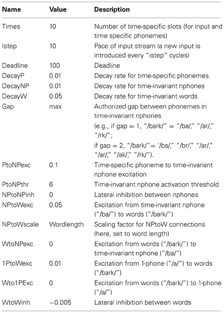
B. Sizing Trace
Recall that TRACE duplicates each feature, phoneme, and word unit at multiple time slices. Features repeat every slice, while phonemes and words repeat every three slices. Figure 2 illustrates reduplication and temporal extent of each unit type. For completeness we will include the feature level in our sizing of TRACE, although it will not be taken into account in our comparison with TISK. In the following, S, F, P, and W will, respectively stand for the number of time slices, features, phonemes and words in the model.
B.1 Counting units
Because there is a bank of F features aligned with every slice, there are SF feature units. For phonemes, given that we have P time-specific units every three slices, for a total of P(S/3). For words, we have W time-specific units every three slices, for a total of W(S/3).
The total number of units as a function of S, F, P, and W can therefore be written: SF + P(S/3) + W(S/3) = S(F + P/3 + W/3) We see that the cost in units is linear in all of these variables, and that for 201 time slices, 212 words, 14 phonemes, and 64 feature units the TRACE model requires 12,633 + 938 + 14,204 = 27,805 units.
B.2 Counting connections
We start by counting the feature-phoneme connections. There are seven features per phoneme on average (vowels, fricatives and liquids don’t use the burst parameter, but some phones take two values within a feature level). Let us count how many phoneme units overlap with each slice. From Figure 2, we can see that two copies of each phoneme overlap with each time slice. Therefore, there are seven (features) *2 (copies) *P feature-phoneme connections per slice, which results in 14 PS feature-phoneme connections in the model.
Let us proceed to phoneme-word and word-phoneme connections. Words are four phonemes long on average, and there are W(S/3) word units. But each of those units receives input not just from the four phonemes that are maximally aligned with it, but also the phonemes to the left and right of the maximally aligned phonemes. Thus, the total number of phoneme-word connections will be 3(S/3)Wp = SWp, where p is the number of phonemes per word. There will be an equal number of feedback connections from words to phonemes, for a total count of 4SW Phoneme-phoneme connections.
Next we consider the phoneme–phoneme connections. Each phoneme unit has an inhibitory link to each phoneme unit with which it overlaps. We can see from Figure 2 that three copies of each phoneme overlap any given slice. So for each phoneme unit aligned at a given slice, it will have 3P − 1 outgoing inhibitory links (we subtract 1 for the unit itself). We do not need to count incoming connections; these are included when we multiply by the number of phoneme units. This results in a total count of PS(P − 1/3) word–word connections.
Just like phonemes, each word unit has an inhibitory link to each word unit with which it overlaps. The number of copies of any word that will overlap with a given slice will vary with word length, as can be seen in Figure 2. We can also see from Figure 2 that words span six slices per phoneme. Recall that words are duplicated every three slices. For the 2- and 3-phoneme long examples in Figure 2, we can determine that the number of copies of each word of length p that overlap with a given third slice (that is, an alignment slice, or a slice where one copy of the word is actually aligned) would be 1 + 2(2p − 1) (the first 1 is for the unit aligned at the slice), i.e., 4p − 1. So a word unit at an alignment slice will have (4p − 1)W − 1 outgoing inhibitory connections. Therefore we arrive at a count of W(S/3)(4p − 1)W − 1) word–word connections, which for an average word length of four phonemes amounts to SW(5W − 1/3). All in all, we arrive at the following formula for the total connection count in TRACE: Total = 14PS + 4SW + PS(P − 1/3) + SW(5W − 1/3) = S(14P + W + P(P − 1/3) + W(5W − 1/3)) = S(P(P + 41/3) + W(5W + 2/3)) = S[(P2 + 41/3P) + (5W2 + 2/3W)].
According to our calculations, the cost in connections is therefore a quadratic function of P and W (due to lateral inhibition at the phoneme and word levels), and a linear function of S (due to limited overlap of units over time slices). In particular, with the standard parameters of 212 words, 14 phonemes, a mean word length of 4 phonemes, and 67 alignment units the TRACE model requires 45,573,266 connections.
C. Sizing Tisk
TISK has three levels: a time specific phoneme level, a time-invariant string kernel level (tisk, after which the model is named), and a time-invariant word level. TISK doesn’t have a feature level, and instead the output of such a level is emulated by a wave of net inputs that arrives to the time-specific phoneme level at a regular pace. A feedforward symmetry network operates the transition between the time-specific phoneme level and the nphone level. There are positive feedforward and feedback connections between the nphone and word levels, and lateral inhibitory connections within them, although in practice only the word level has non-zero inhibitory connections and they are restricted to neighbors. The cuts in computational resources are mostly due to the symmetry network, and to a lesser extent, to the limited use of lateral inhibition.
C.1 TISK units
Because only one level is time-specific in TISK, the notion of alignment doesn’t have course anymore. Therefore the number of time-specific phonemes is simply given by the number of phonemes multiplied by the number of time slices, or PS. With 14 phonemes and, 201 slices, this amounts to 2814 time-specific phoneme units. The nphone level hosts time-invariant phonemes and all possible diphones (even phonotactically illegal ones), and therefore uses P + P2 units, which for P = 14 means 210 units. Finally the word level counts W units, one for each word in the lexicon, and W is set to 212 throughout most simulations. The total number of units in the model is therefore PS + P + P2 + W = P(P + S + 1) + W = 3236 units. W time-invariant word units (212). P + P2 time-invariant n-phone units (P 1-phones and P2 diphones; = 210). Total units at basic parameters: 1360.
C.2 TISK connections
We only count non-zero connections throughout. We start by sizing connections in the symmetry network (Figure 3). A time-specific phoneme unit sends a connection to an nphone unit if and only if it is a constituent of this unit (for instance, A2 sends a connection to A, AB, BA, and AA, but not to B). There are 2P − 1 diphones that start or end with a given phoneme, and one time-invariant phoneme, so a given phoneme at time t will send 2P − 1 + 1 = 2P connections, and multiplying this by the number of time specific phonemes PS, we see that the total number of connections is 2P2S. From this, however, we must remove all zero connections: unit A1 (resp. AT) should not give evidence for diphone units that end with A (resp. that start with A), and therefore gradient coding assigns zero to these connections. We see that these cases only occur at the first and last time slices (implying that there are more than two time slices), and that for a given phoneme, P − 1 connections are concerned, resulting in 2P(P − 1) zero connections. There are therefore 2P2S − 2P(P − 1), or 2P(SP − P + 1), phoneme-to-nphone connections in the symmetry network (with 14 phonemes and 201 time slices, this amounts to 78,428 connections).
We must now count the number of gating connections in the symmetry network. To prevent spurious activations at the nphone level, the symmetry network uses gating connections. These are hard-wired connections that originate from time specific phonemes, and inhibit some connections between time-specific phonemes and time-invariant nphones. Specifically, a given phoneme at a given time slice will inhibit all connections at later time slices that originate from the same phoneme and arrive to a diphone that begins with that phoneme (and does not repeat). Because there are P − 1 diphones that start with a given phoneme and do not repeat, and there are P phonemes at a given time slice, P(P − 1) connections must be gated at any time slice after the one considered, or for S > 2:
With 14 phonemes and 201 time slices, this amounts to 3,658,200 gating units. The total in the time specific part of the network is therefore of 3,658,200 + 78,428 = 3,736,628 connections (Note that the formulas obtained here were verified empirically by direct inspection of the number of connections in the model for various number of time slices, and were found to be exact in all cases). We now proceed to count connections in the time invariant part of the network, first noticing that because lateral inhibition at the nphone level was set to zero, we only need to count the connections between the nphone and the word level, as well as the lateral connections within the word level. However, in TISK these numbers will depend not only on the size of the lexicon and the number of nphones, but critically also on the distribution of nphones in the particular lexicon being used, so that we are reduced to statistical approximations. Empirically, we find that an average word connects to 9.5 nphones in TISK, leading to an estimate of 9.5 W feedforward connections between the nphone and word level. Similarly, simulations show that the number of lateral inhibitory connections at the word level in TISK is 0.8W(W − 1). Therefore the number of connections in the time-invariant part of the model reaches 0.8W2 − 0.8W + 9.6W = 0.8W2 + 8.8W. With a lexicon of 212 words, this amounts to 37,800 connections.
All in all, we arrive at the following expression for the number of connections in TISK for S > 2:
which amounts to 3,774,428 connections using our usual assumptions on S, P, and W. It can be seen when this expression is developed that it is quadratic in S, P, and W. This would seem to be a setback compared to the expression obtained for TRACE, which is only quadratic in P and W but linear in S. However, S is orders of magnitudes smaller than W, and what we obtain in exchange of this quadratic dependence to S is to decouple the S and W factors, reflecting the fact that in TISK the lexicon is not duplicated for every time slice anymore. Consequently there is a substantial gain in connections when switching from TRACE (45,573,266) to TISK (3,774,105) connections, the latter having ten times less connections, a gain of one order of magnitude which improves with lexicon size to reach an asymptota at three orders of magnitude.