
Use sparklines to show data trends
A sparkline is a tiny chart in a worksheet cell that provides a visual representation of data. Use sparklines to show trends in a series of values, such as seasonal increases or decreases, economic cycles, or to highlight maximum and minimum values. Position a sparkline near its data for greatest impact.

Add a Sparkline
-
Select a blank cell at the end of a row of data.
-
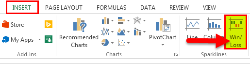
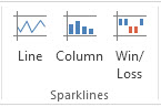
Select Insert and pick Sparkline type, like Line, or Column.
-
Select cells in the row and OK in menu.
-
More rows of data? Drag handle to add a Sparkline for each row.
Format a Sparkline chart
-
Select the Sparkline chart.
-
Select Sparkline and then select an option.
-
Select Line, Column, or Win/Loss to change the chart type.
-
Check Markers to highlight individual values in the Sparkline chart.
-
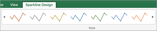
Select a Style for the Sparkline.
-
Select Sparkline Color and the color.
-
Select Sparkline Color > Weight to select the width of the Sparkline.
-
Select Marker Color to change the color of the markers.
-
If the data has positive and negative values, select Axis to show the axis.
-
Need more help?
You can always ask an expert in the Excel Tech Community or get support in the Answers community.
See Also
Analyze trends in data using Sparklines
Get Microsoft chart templates
Need more help?
Sparkline in Excel is a small graph which is used to represent a series of data. Apart from a well-fledged chart, it fits into a single cell. Three different data visualizations available in Excel Sparkline are:
- Line
- Column
- Win/Loss
It is an instant chart that prepares for a range of values. Sparklines in Excel is used to showcase the data trend for a while.
In this Excel Sparklines tutorial, you will learn
- What is Sparklines in Excel
- Why use Sparkline?
- Types of Sparklines in Excel
- How to insert Sparklines in Excel?
- Sparkline Example: Create a Report with a Table
- How to format a Sparklines in Excel
- Advantages of Sparklines in Excel
Why use Sparklines?
Sparkline graph helps you to avoid the chore of creating a big chart which can be confusing during analysis. It is a common visualization technique used in dashboards when you want to picture a portion of data from a large dataset.
Sparklines in Excel is not an object like Excel graphs; it resides in a cell as ordinary data. When you increase the size of the Excel, Sparkline automatically fit into the cells according to its size.
Types of Sparklines in Excel
From the Insert menu, select the type of Sparkline you want. It offers three types of Sparklines in Excel.

- Line Sparkline: Line Sparkline in Excel will be in the form of lines, and high values will indicate fluctuations in height difference.
- Column Sparkline: Column Sparkline in Excel will be in the form of column chart or bar chart. Each bar shows each value.
- Win/Loss Sparkline: It is mainly used to show negative values like ups and downs on the floated costs.

Depending on the type, it gives different visualization to the selected data. Where the line is a tiny chart similar to the line chart, the column is a miniature of bar chart and win/loss resembles waterfall charts.
How to insert Sparklines in Excel?
You need to select a particular column data, to insert Sparklines in Excel.
Consider the following demo data: Status of some pending stock for different years is below. To make a quick analysis, let’s make a Sparkline for each year.
| Year | Jan | Feb | March | April | May | June |
|---|---|---|---|---|---|---|
| 2011 | 20 | 108 | 45 | 10 | 105 | 48 |
| 2012 | 48 | 10 | 0 | 0 | 78 | 74 |
| 2013 | 12 | 102 | 10 | 0 | 0 | 100 |
| 2014 | 1 | 20 | 3 | 40 | 5 | 60 |
Download Excel used on this tutorial
Step 1) Select types of Sparkline
Select the next column to ‘June’ and insert Sparkline from insert menu. Select anyone from the three types of Sparkline.

Step 2) Choose a range of cells
A selection window will appear to select the range of cells for which the Sparkline should insert.
By clicking the arrow near data range box, a range of cells can be choosen.

Step 3) Selected Data Range will be shown
Select the first row of the data for the year 2011 in ‘Data Range’ text box. The range will shown as B2: G2.

Step 4) Choose Location Range
Another range selection indicates where you want to insert the Sparkline. Give the address of the cell you need the Sparkline.

Step 5) Press ‘OK’ Button
Once you set the ‘Data Range’ and ‘Location Range’ press ‘OK’ button.

Step 6) Sparkline is created in the selected cell
Now the Sparkline is created for the selected data, and it gets inserted in the selected cell H3.

Sparkline Example: Create a Report with a Table
You have a sales report for four years: 2015, 2016, 2017 respectively. Details included in this table are country, product, and gross sales.
Let’s find the trend of sales for this product for different years.
Step 1) Create a column analysis next to gross sales for 2018. And in the next step, you are going to insert the Sparkline.
| S# | Country | Product | Gross Sales 2015 | Gross Sales 2016 | Gross Sales 2017 | Gross Sales 2018 |
|---|---|---|---|---|---|---|
| 1 | Canada | Carretera | $ 32,370.00 | $ 30,216.00 | $ 352,625.00 | $ 34,440.00 |
| 2 | Germany | Carretera | $ 26,420.00 | $ 352,100.00 | $ 43,125.00 | $ 7,210.00 |
| 3 | France | Carretera | $ 32,670.00 | $ 4,404.00 | $ 600,300.00 | $ 4,473.00 |
| 4 | Singapore | Carretera | $ 13,320.00 | $ 6,181.00 | $ 34,056.00 | $ 9,282.00 |
| 5 | United States of America | Carretera | $ 37,050.00 | $ 8,235.00 | $ 32,670.00 | $ 22,296.00 |
| 6 | Mexico | Carretera | $ 529,550.00 | $ 236,400.00 | $ 13,320.00 | $ 423,500.00 |
| 7 | China | Carretera | $ 13,815.00 | $ 37,080.00 | $ 534,450.00 | $ 17,703.00 |
| 8 | Spain | Carretera | $ 30,216.00 | $ 8,001.00 | $ 645,300.00 | $ 17,340.00 |
| 9 | Japan | Carretera | $ 37,980.00 | $ 603,750.00 | $ 36,340.00 | $ 41,250.00 |
| 10 | Korea (Republic of) | Carretera | $ 18,540.00 | $ 10,944.00 | $ 962,500.00 | $ 32,052.00 |
| 11 | Italy | Carretera | $ 37,050.00 | $ 32,280.00 | $ 23,436.00 | $ 9,192.00 |
| 12 | Costa Rica | Carretera | $ 333,187.50 | $ 36,340.00 | $ 527,437.50 | $ 148,200.00 |
| 13 | Taiwan | Carretera | $ 287,400.00 | $ 529,550.00 | $ 37,980.00 | $ 488,950.00 |
| 14 | Argentina | Carretera | $ 15,022.00 | $ 10,451.00 | $ 11,802.00 | $ 754,250.00 |
| 15 | Denmark | Carretera | $ 43,125.00 | $ 225,500.00 | $ 25,692.00 | $ 33,210.00 |
| 16 | Belgium | Carretera | $ 9,225.00 | $ 25,932.00 | $ 8,001.00 | $ 690,300.00 |
Step 2) Select the cell in which you want to insert the Sparkline. Go to Insert menu from the menu bar. Select any one of the Sparkline from the list of Sparkline.

Step 3) Select any one of the sparkline types that you want to insert. It will ask for the range of cells. Select the line type from the available sparkline type.
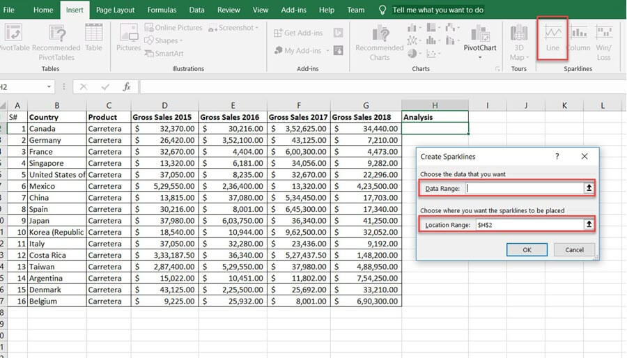
Data Range indicates, which data the Sparkline need to insert. Location range is the cell address where you want to add the Sparkline.
Step 4) Here, the data range is from the cell data contains ‘Gross sales 2015 to 2018’ and location range is from H3. Press the ‘OK’ button after this.

Step 5) The Sparkline will be inserted into the H3 cell. You can apply the Sparkline to entire data by dragging the same to downwards.

Now the Sparkline is created.
How to format a Sparklines in Excel
To format Sparkline, first Click on the created Sparkline. A new tab named design will appear on the menu bar which includes the Sparkline tools and will help you to change its color and style. See the available options one by one.

The different properties of Sparkline can customize according to your need. Style, color, thickness, type, the axis is some among them.
How to change the style of the Sparklines?
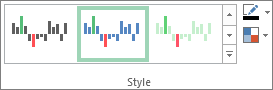
Step 1) Select a style from the ‘Style’ option within the design menu. The styles included in a dropdown.

Step 2) Click on the down arrow near to the style option to select your favorite style from an extensive design catalog.

How to change the color of the Sparklines?
The color and thickness of the Sparkline can be changed using the Sparkline Color option. It offers a variety of colors.
Step 1) Select the Sparkline and select the Sparkline Color option from the design menu.

Step 2) Click on the color you want to change. The Sparkline will update with the selected color.

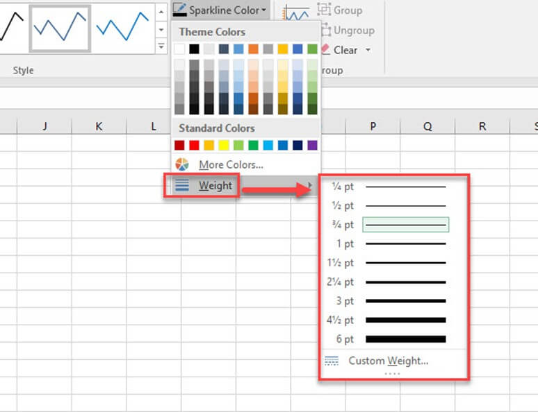
Change the width of lines.
The width of the lines can be adjusted with the option available in the ‘Sparkline Color’ window.
Step 1) Select the Sparkline then go to design menu in the menu bar.
Step 2) Click on the Sparkline Color’ option.
Step 3) Select the Weight option to make changes in thickness to the inserted Sparkline.

Step 4) Move to Weight option. This will give a list of predefined thickness. Customization in Weight is also available.
Highlighting the data points
You can highlight the highest, lowest points, and the entire data points on a Sparkline. By this you to get a better view of the data trend.
Step 1) Select the created Sparkline in any cell then move to the design menu. You can see different checkboxes to highlight the data points.

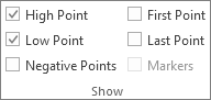
Step 2) Give checkmark according to the data points you want to highlight. And the options available are:
- High/Low Point: Highlights the high spot the high and low points on the Sparkline.
- First/Last Point: This will help to highlight the first and last data points on the Sparkline.
- Negative Points: Use this to highlight negative values.
- Markers: This option applies only to line Sparkline. It will highlight all data points with a marker. Different color and style are available with more marker colors and lines.

Deleting the Sparklines
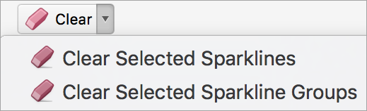
You can’t remove the Sparkline by hitting the ‘delete’ key on a keyboard. To delete the Sparkline, you should go to the ‘Clear’ option.
Step 1) Select the cell, which included the Sparkline.
Step 2) Go to Sparkline tools design menu.
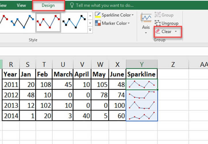
Step 3) Click on the clear option this will delete the selected Sparkline from the cell.
Advantages of Sparklines in Excel
Here are important reasons for using Sparkline:
- Visualization of data like temperature or stock market price.
- Transforming data into a compact form.
- Data reports generating for a short time.
- Analyze data trends for a particular time.
- Easy to understand the fluctuations in the data.
- A better understanding of high and low data points.
- Negative values can float effectively by sparkline.
- Sparkline automatically adjusts its size once the cell width is changed.
Summary
- Sparkline is a small chart which does not recommend an axes or coordinates
- Sparkline can apply on a single column or row of data series.
- Different formatting properties are available for the Sparkline.
- Sparkline is a micrograph which fit into a single cell.
- A single delete key press will not remove a created Sparkline.
- The different data points can highlight in a Sparkline.
Sparklines feature was introduced in Excel 2010.
In this article, you’ll learn all about Excel Sparklines and see some useful examples of it.
What are Sparklines?
Sparklines are tiny charts that reside in a cell in Excel. These charts are used to show a trend over time or the variation in the dataset.
You can use these sparklines to make your bland data look better by adding this layer of visual analysis.
While Sparklines are tiny charts, they have limited functionality (as compared with regular charts in Excel). Despite that, Sparklines are great as you can create these easy to show a trend (and even outliers/high-low points) and make your reports and dashboard more reader-friendly.
Unlike regular charts, Sparklines are not objects. These reside in a cell as the background of that cell.
Types of Sparklines in Excel
In Excel, there are three types of sparklines:
- Line
- Column
- Win-loss
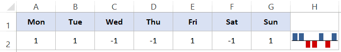
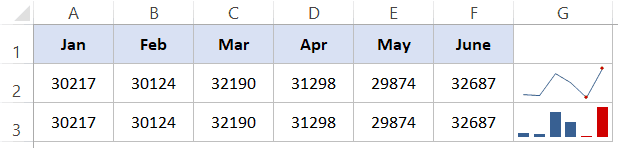
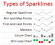
In the below image, I have created an example of all these three types of sparklines.
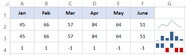
The first one in G2 is a line type sparkline, in G3 is a column type and in G4 is the win-loss type.
Here are a few important things to know about Excel Sparklines:
- Sparklines are dynamic and are dependent on the underlying dataset. When the underlying dataset changes, the sparkline would automatically update. This makes it a useful tool to use when creating Excel dashboards.
- Sparklines size is dependent on the size of the cell. If you change the cell height or width, the sparkline would adjust accordingly.
- While you have sparkline in a cell, you can also enter a text in it.
- You can customize these sparklines – such as change the color, add an axis, highlight maximum/minimum data points, etc. We will see how to do this for each sparkline type later in this tutorial.
Note: A Win-loss sparkline is just like a column sparkline, but it doesn’t show the magnitude of the value. It is better used in situations where the outcome is binary, such as Yes/No, True/False, Head/Tail, 1/-1, etc. For example, if you’re plotting whether it rained in the past 7 days or not, you can plot a win-loss with 1 for days when it rained and -1 for days when it didn’t. In this tutorial, everything covered for column sparklines can also be applied to the win-loss sparklines.
Now let’s cover each of these types of sparklines and all the customizations you can do with it.
Inserting Sparklines in Excel
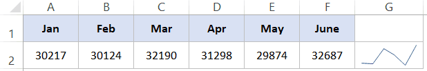
Let’s say that you want to insert a line sparkline (as shown below).
Here are the steps to insert a line sparkline in Excel:
- Select the cell in which you want the sparkline.
- Click on the Insert tab.

- In the Sparklines group click on the Line option.

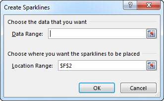
- In the ‘Create Sparklines’ dialog box, select the data range (A2:F2 in this example).

- Click OK.


This will insert a line sparkline in cell G2.
To insert a ‘Column’ or ‘Win-loss’ sparkline, you need to follow the same above steps, and select Columns or Win-loss instead of the Line (in step 3).
While the above steps insert a basic sparkline in the cell, you can do some customization to make it better.
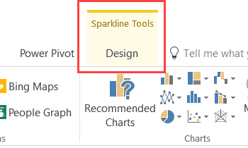
When you select a cell that has a Sparkline, you’ll notice that a contextual tab – Sparkline Tools Design – becomes available. In this contextual tab, you’ll find all the customization option for the selected sparkline type.
Editing the DataSet of Existing Sparklines
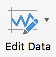
You can edit the data of an existing sparkline by using the Edit Data option. When you click on the Edit Data drop down, you get the following options:
- Edit Group Location & Data: Use this when you have grouped multiple sparklines and you want to change the data for the entire group (grouping is covered later in this tutorial).
- Edit Single Sparkline’s Data: Use this to change the data for the selected sparkline only.
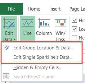
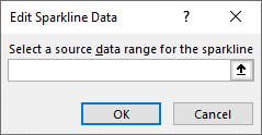
Clicking on any of these options open the Edit Sparklines dialog box where you can change the data range.
Handling Hidden and Empty Cells
When you create a line sparkline with a dataset that has an empty cell, you will notice that the sparkline shows a gap for that empty cell.
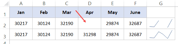
In the above dataset, the value for April is missing which creates a gap in the first sparkline.
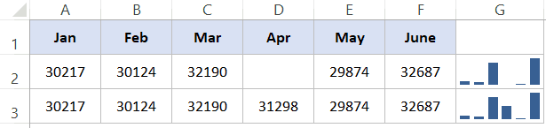
Here is an example where there is a missing data point in a column sparkline.
You can specify how you want these empty cells to be treated.
Here are the steps:
- Click the cell that has the sparkline.
- Click the Design Tab (a contextual tab that becomes available only when you select the cell that has a sparkline).
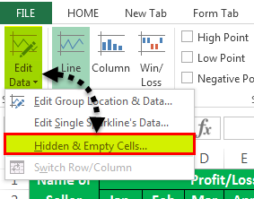
- Click on the Edit Data option (click on the text part and not the icon of it).
- In the drop-down, select ‘Hidden & Empty Cells’ option.

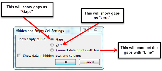
- In the dialog box that opens, select whether you want to show
- Empty cells as gaps
- Empty cells as zero
- Connect the before and after data points with a line [this option is available for line sparklines only].


In case the data for the sparkline is in cells that are hidden, you can check the ‘Show data in hidden rows and columns’ to make sure the data form these cells is also plotted. If you don’t do this, data from hidden cells will be ignored.
Below is an example of all three options for a line sparkline:
- Cell G2 is what happens when you choose to show a gap in the sparkline.
- Cell G3 is what happens when you choose to show a zero instead.
- Cell G2 is what happens when you choose to show a continuous line by connecting the data points.
You can do the same with column and win-loss sparklines as well (not the connecting data point option).
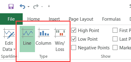
Changing the Sparkline Type
If you want to quickly change the sparkline type – from line to column or vice versa, you can do that using the following steps:
- Click the sparkline you want to change.
- Click the Sparkline Tools Design tab.
- In the Type group, select the sparkline you want.
Highlighting Data Points in Sparklines
While a simple sparkline shows the trend over time, you can also use some markers and highlights to make it more meaningful.
For example, you can highlight the maximum and the minimum data points, first and the last data point, as well as all the negative data points.
Below is an example where I have highlighted the maximum and minimum data points in a line and column sparkline.
These options are available in the Sparkline Tools tab (in the show group).
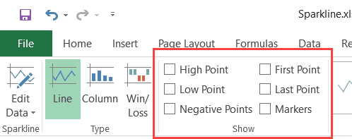
Here are the different options available:
- High/Low Point: You can use any one or both of these to highlight the maximum and/or the minimum data point.
- First/Last Point: You can use any one or both of these to highlight the first and/or the last data point.
- Negative Points: In case you have negative data points, you can use this option to highlight all of these at once.
- Markers: This option is available only for line sparklines. It will highlight all the data points with a marker. You can change the color of the marker using the ‘Marker Color’ option.
Sparklines Color and Style
You can change the way sparklines look using the style and color options.
It allows you to change the sparkline color (of lines or columns) as well as the markers.
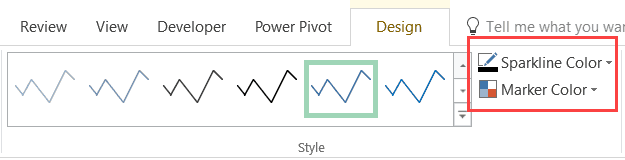
You can also use the pre-made style options. To get the full list of options. click on the drop-down icon in the bottom-right of the style box.
![]()
Pro Tip: If you’re are using markers to highlight certain data points, it’s a good idea to choose a line color that is light in color and marker that is bright and dark (red works great in most cases).
Adding an Axis
When you create a sparkline, in its default form, it shows the lowest data point at the bottom and all the other data points are relative to it.
In some cases, you may not want this to be the case as it seems to show a huge variation.
In the below example, the variation is only 5 points (where the entire data set is between 95 and 100). But since the axis starts from the lowest point (which is 95), the variation looks huge.
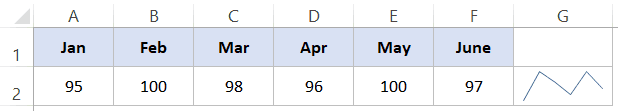
This difference is a lot more prominent in a column sparkline:
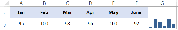
In the above column sparkline, it may look like the Jan value is close to 0.
To adjust this, you can change the axis in the sparklines (make it start at a specific value).
Here is how to do this:
- Select the cell with the sparkline(s).
- Click on the Sparkline Tools Design tab.
- Click on the Axis option.

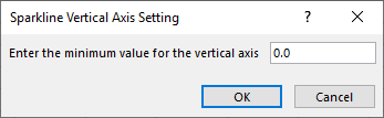
- In the drop-down, select Custom Value (in the Vertical Axis Minimum Value Options).

- In the Sparkline Vertical Axis Settings dialog box, enter the value as 0.

- Click OK.


This will give you the result as shown below.
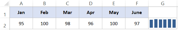
By setting the customs value at 0, we have forced the sparkline to start at 0. This gives a true representation of the variation.
Note: In case you have negative numbers in your data set, it’s best to not set the axis. For example, if you set the axis to 0, the negative numbers would not be shown in the sparkline (as it begins from 0).
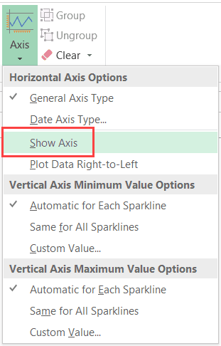
You can also make the axis visible by selecting the Show Axis option. This is useful only when you have numbers that cross the axis. For example, if you have the axis set at 0 and have both positive and negative numbers, then the axis would be visible.
Group & Ungroup Sparklines
If you have a number of sparklines in your report or dashboard, you can group some of these together. Doing this makes it easy to make changes to the whole group instead of doing it one by one.
To group Sparklines:
- Select the ones that you want to group.
- Click on the Sparklines Tools Design tab.
- Click the Group icon.


Now when you select any of the Sparkline that has been grouped, it will automatically select all the ones in that group.
You can ungroup these sparklines by using the Ungroup Option.
Deleting the Sparklines
You can not delete a sparkline by selecting the cell and hitting the delete key.
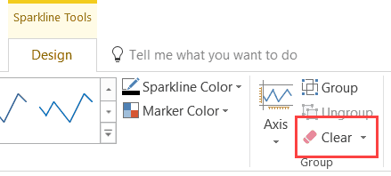
To delete a sparkline, follow the steps below:
- Select the cell that has the sparkline that you want to delete.
- Click the Sparkline Tools Design tab.
- Click the Clear option.
You May Also Like the Following Excel Tutorials:
- Using Conditional Formatting in Excel (The Ultimate Guide + Examples).
- How to Create a Heat Map in Excel.
- Creating the Actual vs Target Chart in Excel.
- Sparklines in Google Sheets
- How to Rotate Text in Cells in Excel
Sparklines are tiny charts inside single worksheet cells that can be used to visually represent and show a trend in your data. Sparklines can draw attention to important items such as seasonal changes or economic cycles and highlight the maximum and minimum values in a different color.
Contents
- 1 What are sparklines and their purpose?
- 2 What are the three types of sparklines in Excel?
- 3 How do I create a sparkline in Excel?
- 4 What is the difference between sparklines and charts in Excel?
- 5 Are sparklines useful?
- 6 For what purpose MS Excel is used?
- 7 What are different types of sparklines?
- 8 What does macro mean in Excel?
- 9 What is combo chart?
- 10 What is the best use for a sparkline?
- 11 How do I know if Excel is compatible?
- 12 What is chart and diagram?
- 13 What is a splunk sparkline?
- 14 Why is it called a sparkline?
- 15 What is the disadvantage of stacked area charts?
- 16 How many cells in your worksheet does a sparkline use?
- 17 Why would you not use a sparkline?
- 18 What are the 3 common uses for Excel?
- 19 What are the advantages of MS Excel?
- 20 How do you show markers in Excel?
What are sparklines and their purpose?
Sparklines are small graphs that are created to offer simple visual clues about the data graphed. Basically, they are tiny charts inside a single cell.
What are the three types of sparklines in Excel?
There are three types of sparklines:
- Line: visualizes the data in a line graph form.
- Column: visualizes the data in column form, similar to the clustered column chart.
- Win/Loss: visualizes the data as positive or negative based on color.
How do I create a sparkline in Excel?
Here are the steps to insert a line sparkline in Excel:
- Select the cell in which you want the sparkline.
- Click on the Insert tab.
- In the Sparklines group click on the Line option.
- In the ‘Create Sparklines’ dialog box, select the data range (A2:F2 in this example).
- Click OK.
What is the difference between sparklines and charts in Excel?
A sparkline is a very small line chart, typically drawn without axes or coordinates.Whereas the typical chart is designed to show as much data as possible, and is set off from the flow of text, sparklines are intended to be succinct, memorable, and located where they are discussed.
Are sparklines useful?
Excel Sparklines provide an easy way to add lightweight graphics to your data. A Sparkline chart is a good choice for summarizing data within a row of a table. They typically will be placed in the same row, to the right of the data.
For what purpose MS Excel is used?
Microsoft Excel is a spreadsheet program. That means it’s used to create grids of text, numbers and formulas specifying calculations. That’s extremely valuable for many businesses, which use it to record expenditures and income, plan budgets, chart data and succinctly present fiscal results.
What are different types of sparklines?
There are three different types of sparklines: Line, Column, and Win/Loss. Line and Column work the same as line and column charts.
What does macro mean in Excel?
If you have tasks in Microsoft Excel that you do repeatedly, you can record a macro to automate those tasks. A macro is an action or a set of actions that you can run as many times as you want. When you create a macro, you are recording your mouse clicks and keystrokes.
What is combo chart?
A combo chart is a combination of two column charts, two line graphs, or a column chart and a line graph. You can make a combo chart with a single dataset or with two datasets that share a common string field.
What is the best use for a sparkline?
A sparkline is a tiny chart in a worksheet cell that provides a visual representation of data. Use sparklines to show trends in a series of values, such as seasonal increases or decreases, economic cycles, or to highlight maximum and minimum values. Position a sparkline near its data for greatest impact.
How do I know if Excel is compatible?
Follow these steps:
- Click File > Info > Check for Issues.
- Choose Check Compatibility.
- To check for compatibility automatically from now on, check the Check compatibility when saving this workbook box. Tip: You can also specify the versions of Excel that you want to include when you check for compatibility.
What is chart and diagram?
As nouns the difference between diagram and chart
is that diagram is a plan, drawing, sketch or outline to show how something works, or show the relationships between the parts of a whole while chart is a map.
What is a splunk sparkline?
A sparkline is a small representation of some statistical information without showing the axes. It generally appears as a line with bumps just to indicate how certain quantity has changed over a period of time. Splunk has in-built function to create sparklines from the events it searches.
Why is it called a sparkline?
Sparklines are often used in reports, presentations, dashboards and scoreboards. They do not include axes or labels; context comes from the related content. Usually, when a graph is included in a report, the reader has to break concentration and take time to study the graph.
What is the disadvantage of stacked area charts?
There’s nothing stopping us from breaking up this one graph into smaller individual graphs, one for each and also the total. The disadvantage here is that it’s not as easy to compare between the different groups, however we can make it easier by using the same axis scaling for the graphs for each individual group.
How many cells in your worksheet does a sparkline use?
Sparklines in Excel are graphs that fit in one cell. Sparklines are great for displaying trends.
Why would you not use a sparkline?
The line sparkline displays data values in a line chart. The column sparkline displays values using a column chart.You would not use a sparkline if you need to show specific details in your chart or need to augment the informative chart elements.
What are the 3 common uses for Excel?
The three most common general uses for spreadsheet software are to create budgets, produce graphs and charts, and for storing and sorting data. Within business spreadsheet software is used to forecast future performance, calculate tax, completing basic payroll, producing charts and calculating revenues.
What are the advantages of MS Excel?
10 Benefits of Microsoft Excel
- Best way to store data.
- You can perform calculations.
- All the tools for data analysis.
- Easy to data visualizations with charts.
- You can print reports easily.
- So many free templates to use.
- You can code to automate.
- Transform and clean data.
How do you show markers in Excel?
On the Format tab, in the Current Selection group, click Format Selection. Click Marker Options, and then under Marker Type, make sure that Built-in is selected. In the Type box, select the marker type that you want to use.
What are the Sparklines in Excel?
Sparklines in Excel are like a chart in a cell itself. They are tiny visual representations that show the trend of the data, increasing or decreasing. So first, we need to select the cell where we want the sparkline to insert a sparkline. Then, in the “Insert” tab in the “Lines” section, click on “Sparklines.” After that, we can choose any one of the styles of sparklines.
Sparklines are most useful when multiple charts are required to represent the data. It is because the chart will take up most of the spreadsheet space. We can save this space by using sparklines in Excel.
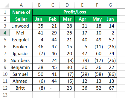
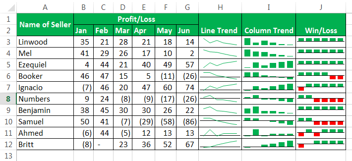
Suppose we have the profit and loss data for the first two quarters of 10 sellers. We want to visualize the trend of profit or loss they make in two quarters. Then, we cannot do this with the help of single traditional charts. It can be possible only if sparklines are inserted for each seller.
Table of contents
- What are the Sparklines in Excel?
- How to Create Sparklines in Excel?
- Example #1 – Using Column
- Example #2 – Using Win/Loss
- Example #3 – If in case we have Blank cells or zero value cells in the data
- Explanation
- Things to Remember
- Recommended Articles
- How to Create Sparklines in Excel?
How to Create Sparklines in Excel?
You can download this Sparklines Excel Template here – Sparklines Excel Template
Example #1 – Using Column
Step 1: Since we are creating a column in sparkline this time, we must select the column instead of a line from the available options.
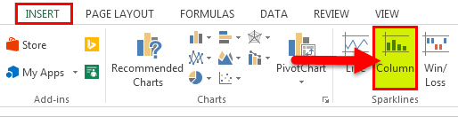
By creating a sparkline, we meant we needed to insert something in Excel. So, whenever we need to insert or add something, we also need to go to the “Insert” tab of Excel.
- So first, we need to go to the “Insert” tab.
Go to the “INSERT” option from the ribbon and choose the “Line” chart from the “Sparklines” options.

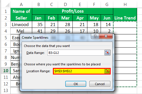
- From the window, enter or select the “Data Range” that has the data.

- Enter the location of the cell where the sparkline is to be created. It is not usually asked when creating a chart, as a chart is an object. But, sparkline is not an object and needs a location to insert in Excel.
- After the location from where the data has to be picked and the location of a cell in which the sparkline is to be inserted. We will get the below sparkline.
Since we have selected the “Line” method for creating a sparkline, the sparkline will be identical to the “Line” chart.


Steps 2 and 3 will be the same as in the case of “Using a line in the sparkline.”
Step 4: The column “Sparkline” will look as below.

Example #2 – Using Win/Loss
Step 1: Select the “Win/Loss” from the available “Sparklines” options.
Steps 2 and 3 will be the same as explained before.
Step 4: The “Win/Loss” sparkline will look like the one below.

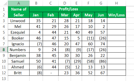
Example #3 – If in case we have Blank cells or zero value cells in the data
If we have blank cells in the data, the sparklines will be broken and look separated as below.

To correct this situation, we need to change how sparkline treats the empty cell.
Step 1: Select the “Sparkline” and click the “Insert” option. From the “Design” tab, select the “Edit Data” option.
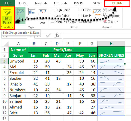
Step 2: From the “Edit Data” option, choose the option “Hidden & Empty Cells.”
Step 3: We can choose how the gaps will be treated from the available options.
Step 4: Below is how each of the options will treat gaps.

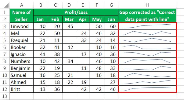
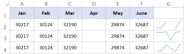
If the data has a gap, it makes broken sparklines. Follow the same steps of the method (1,2, and 3). Below are examples of broken sparklines.
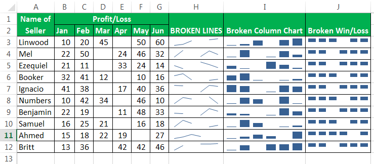
To make a “Markers” in the sparklines, go to the “Design” tab and click on the option “Markers” after inserting sparklines.
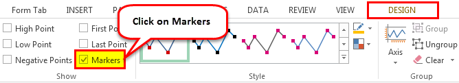
Then, your marker-added sparklines would look like this.

To show the axis in sparklines, go to the “Design” tab and click on “Axis,” then click on “Show Axis.”
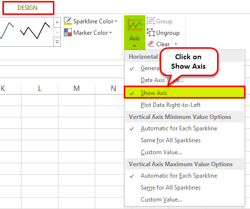
The axis added sparklines would look as given below.
Explanation
When we only need the visualization instead of the full features of traditional charts. We should use sparklines instead of charts as they also have many features that are enough to visualize the data.
Sparklines work the same as a chart, but the only difference is that sparklines are inserted in the cell, and a chart is always outside a cell and is an object to Excel. Getting started with a sparkline is easy as this needs the data to be selected and then insert a sparkline from the ribbon. When we create a sparkline, we have many options about how the sparklines are to be represented. Hence, we can use lines, columns, or win-loss methods. If we use the line sparkline, our chart will be more identical to the line chart. In the case of column chart sparkline, this will match the traditional column chart in excelColumn chart is used to represent data in vertical columns. The height of the column represents the value for the specific data series in a chart, the column chart represents the comparison in the form of column from left to right.read more.
We should remember that we can use the column and line chart if we have data. However, we need to show the change in the magnitude of that data via sparkline. We cannot use the “Win/Loss” type if we want to show the importance of change in data, as this type of chart works on the “True” or “False” method only. Therefore, they cannot show a difference in the magnitude of data.
Things to Remember
- The sparklines are not an object. Therefore, these are inserted into a cell and not on the worksheet area, as done in the case of charts that are inserted as an object and on the worksheet.
- Even if a sparkline is created in a cell, we can still type in that cell.
- A sparkline must be deleted from the menu and cannot be deleted with the click of the “Delete” button.
- The height and width of the sparkline depend on the height and width of the cell in which it is inserted. Therefore, the sparkline look will change if any change is made to the cell’s width and height.
- We should not use the “Win/loss” method of sparkline if we need to show the magnitude of change because they represent the “True” and “False” situations.
Recommended Articles
This article is a guide to Sparklines in Excel. Here, we discuss how to create sparklines in Excel using sparkline options such as “Line,” “Column,” “Win/Loss,” “Marker,” “Broken Lines,” and “Axis,” along with practical examples and downloadable Excel templates. You may learn more about Excel from the following articles: –
- Line Chart ExamplesThe line chart is a graphical representation of data that contains a series of data points with a line. read more
- Dynamic Chart in ExcelA dynamic chart is a unique chart in Excel which updates itself when the range of the chart is updated. In static charts, the chart does not change itself when the range is updated.read more
- Stacked Column Chart in ExcelA stacked column chart in Excel is a column chart where multiple series of the data representation of various categories are stacked over each other. The stacked series are vertical.read more
- Histogram FormulaA histogram is a type of graphical representation in excel, and there are various methods to make one. Instead of using the Analysis Toolpak or from the Pivot Table, we can also make a histogram from formulas, such as using FREQUENCY and Countifs formulas together.read more
Excel is a great tool for all of your marketing needs. You can create graphs to visualize your data, use formulas to calculate conversion rates, or even create social media calendars.

You can also monitor trends in your marketing campaign data and, in this post, we’ll explain how to do so with the sparklines tool.
Already know what you need? Jump there with our Table of Contents.
- How to Add a Sparkline in Excel
- Create a Column Sparkline in Excel
- How to Ungroup Sparklines in Excel
- How to Mark Data Points in Sparkline Charts
- How to Color Code Excel Sparkline
![Download 10 Excel Templates for Marketers [Free Kit]](https://no-cache.hubspot.com/cta/default/53/9ff7a4fe-5293-496c-acca-566bc6e73f42.png)
What are sparklines in Excel?
Sparklines are charts in individual cells that provide visual representations of trends in your sheet data. For example, if you track month-over-month progress, a sparkline can show you how each month compares to the other.
There are three different sparklines you can add to your Excel spreadsheets: line, column, and win-loss. The image below is an example of a line.

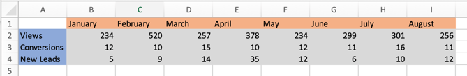
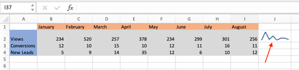
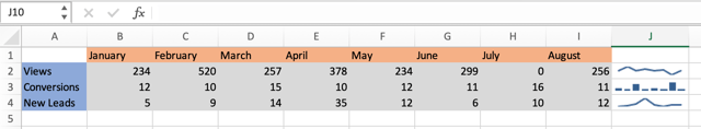
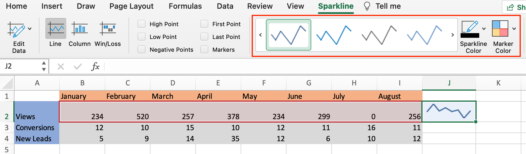
For this walkthrough, we’ll use a sample data table (shown below) that tracks views, conversions, and leads generated from a marketing campaign.
Let’s go over how to add your own.
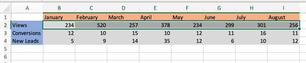
1. Select the cells you want represented in your sparkline chart. In this example, I’ve selected all the cells between B2 and I2.
2. In the header toolbar, select Insert, then Sparklines.
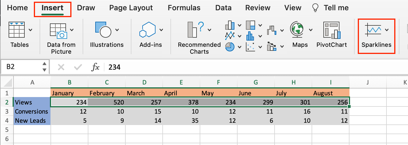
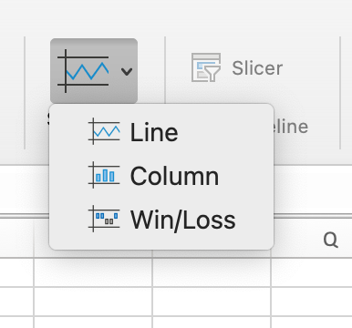
3. You should then see a dropdown menu where you can select the type of sparkline chart you want: line, column, or win-loss. I selected a line for this example.
4. After you select your preferred chart, you’ll see a dialogue box appear (as shown below). In the Select where you want to place the sparkline box text field, enter the cell that you want the sparkline chart in.
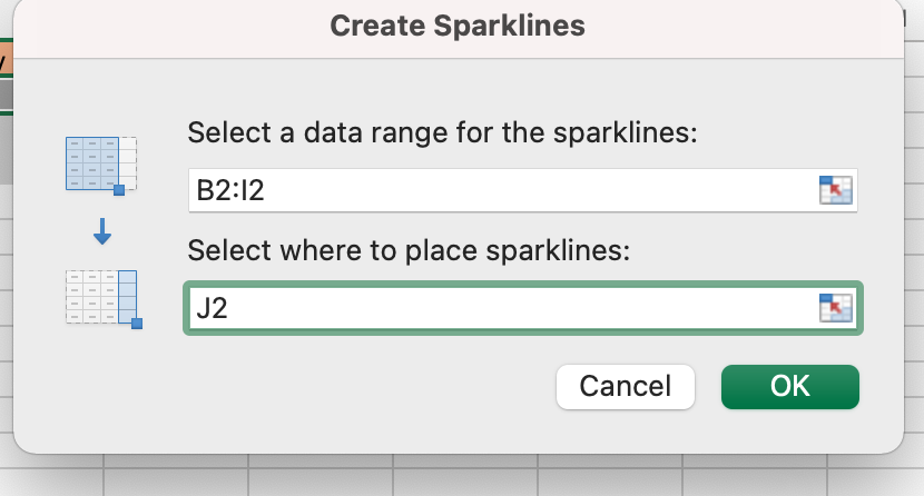
It’s best practice to have the sparkline immediately next to the string of cells you’re creating the chart for so you can get a full visualization and quickly refer back to your data.
For this example, I selected cell J2.
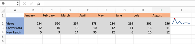
5. Your sparkline chart should appear in the cell you selected. The image below is the sparkline for my sample data set, and it shows the trend in views over time for my marketing campaign.
 Below we’ll go over the steps to creating a different type of sparkline.
Create a Column Sparkline in Excel
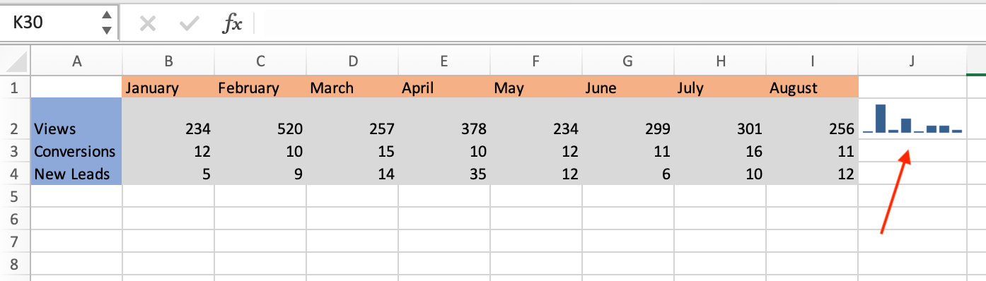
If you want to use a column sparkline in Excel, repeat steps one and two from above. When the sparkline selection box opens, select column instead of line. The image below is a column sparkline.
 Follow the same process if you want a win-loss sparkline. The image below is an example of what this chart looks like.
How to Ungroup Sparklines in Excel
You’d want to ungroup sparklines in Excel if you want each of your rows to have a different sparkline. For example, if you want rows two and four to have a line chart, but row three to have a column. Let’s go over the steps.
1. Right-click on the sparkline you want ungrouped. For this example, I right-clicked on column J3.
2. In the popup menu, select Sparklines, then Ungroup.
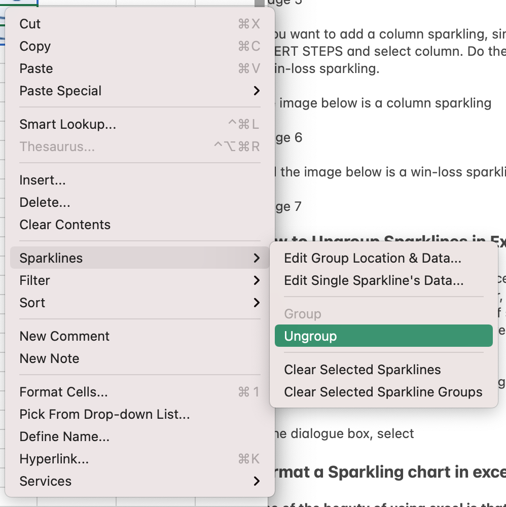
3. Click on the sparkline you want to change, navigate to the Sparkline header toolbar, and make your chart selection.
The image below is an example of what it looks like when you ungroup sparklines and use different charts.
Format a Sparkline Chart in Excel
A benefit to using Excel is that you can always format your spreadsheets to your liking, and this goes for Sparklines too. Let’s go over some formatting changes you can make.
How to Mark Data Points in Sparkline Charts
1. Select the sparkline you want to edit and navigate to the Sparkline header toolbar and select your preferred data marker, as shown in the image below.
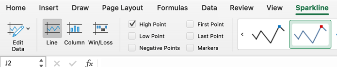
If I select High Point, my corresponding sparkline chart will have a marker displaying the month with the highest view count.
How to Color Code Excel Sparkline
Select the sparkline you want to edit and navigate to the right-hand side of the Sparkline header toolbar, as shown in the image below.
 You have the option to change the color of your sparkline, the color of your markers, and the weight of your sparkline.
Over To You
Now that you know how to create a sparkline chart, you can expertly monitor trends in your marketing campaigns that will help you quickly view the success of your processes.

Содержание
- Use sparklines to show data trends
- Add a Sparkline
- Format a Sparkline chart
- Need more help?
- Analyze trends in data using sparklines
- Customize your sparklines
- Create sparklines
- Create sparklines
- Mark data points on sparklines
- Change the style of sparklines
- Handle empty or zero value cells
- Delete sparklines
- Create sparklines
- Mark data points on sparklines
- Change the style of sparklines
- Handle empty or zero value cells
- Delete sparklines
- What Are Excel Sparklines?
- What are sparklines and their purpose?
- What are the three types of sparklines in Excel?
- How do I create a sparkline in Excel?
- What is the difference between sparklines and charts in Excel?
- Are sparklines useful?
- For what purpose MS Excel is used?
- What are different types of sparklines?
- What does macro mean in Excel?
- What is combo chart?
- What is the best use for a sparkline?
- How do I know if Excel is compatible?
- What is chart and diagram?
- What is a splunk sparkline?
- Why is it called a sparkline?
- What is the disadvantage of stacked area charts?
- How many cells in your worksheet does a sparkline use?
- Why would you not use a sparkline?
- What are the 3 common uses for Excel?
- What are the advantages of MS Excel?
- How do you show markers in Excel?
Use sparklines to show data trends
A sparkline is a tiny chart in a worksheet cell that provides a visual representation of data. Use sparklines to show trends in a series of values, such as seasonal increases or decreases, economic cycles, or to highlight maximum and minimum values. Position a sparkline near its data for greatest impact.
Add a Sparkline
Select a blank cell at the end of a row of data.
Select Insert and pick Sparkline type, like Line, or Column.
Select cells in the row and OK in menu.
More rows of data? Drag handle to add a Sparkline for each row.
Format a Sparkline chart
Select the Sparkline chart.
Select Sparkline and then select an option.
Select Line, Column, or Win/Loss to change the chart type.
Check Markers to highlight individual values in the Sparkline chart.
Select a Style for the Sparkline.
Select Sparkline Color and the color.
Select Sparkline Color > Weight to select the width of the Sparkline.
Select Marker Color to change the color of the markers.
If the data has positive and negative values, select Axis to show the axis.
Need more help?
You can always ask an expert in the Excel Tech Community or get support in the Answers community.
Источник
Analyze trends in data using sparklines
Sparklines are tiny charts inside single worksheet cells that can be used to visually represent and show a trend in your data. Sparklines can draw attention to important items such as seasonal changes or economic cycles and highlight the maximum and minimum values in a different color. Showing trends in your worksheet data can be useful, especially when you’re sharing your data with other people.
Select a blank cell near the data you want to show in a sparkline.
On the Insert tab, in the Sparklines group, click Line, Column, or Win/Loss.
In the Data Range box, enter the range of cells that has the data you want to show in the sparkline.
For example, if your data is in cells A, B, C, and D of row 2, enter A2:D2.
If you’d rather select the range of cells on the worksheet, click  to temporarily collapse the dialog box, select the cells on the worksheet, and then click
  to show the dialog box in full.
The Sparkline Tools appear on the ribbon. Use the Style tab to customize your sparklines.
Because a sparkline is embedded in a cell, any text you enter in the cell uses the sparkline as its background, as shown in the following example.
If you select one cell, you can always copy a sparkline to other cells in a column or row later by dragging or using Fill Down (Ctrl+D).
Customize your sparklines
After you create sparklines, you can change their type, style, and format at any time.
Select the sparklines you want to customize to show the Sparkline Tools on the ribbon.
On the Style tab, pick the options you want. You can:
Show markers to highlight individual values in line sparklines.
Change the style or format of sparklines.
Show and change axis settings.

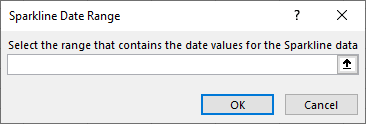
If you click the Date Axis Type option in this drop-down, Excel opens the Sparkline Date Range dialog box. From here, you can select the range in your workbook that contains the date values you want for your Sparkline data.
If you click the Custom Value options in this drop-down, Excel opens the Sparkline Vertical Axis Setting dialog box. From here, you can enter either the minimum or maximum value (depending upon which option you selected) for the vertical axis for your Sparkline data. By default, Excel determines how to display the Sparkline data so with these options you can control the minimum and maximum values.
Change the way data is shown.

If you click the Edit Single Sparkline’s Data option in this drop-down, Excel opens the Edit Sparkline Data dialog box. From here, you can select the range in your workbook that contains the data you want for your Sparkline data. Use this option if you want to change only one Sparkline.
If you click the Hidden & Empty Cells option in this drop-down, Excel opens the Hidden and Empty Cell Settings dialog box. Use this option to change how Excel treats hidden and null values for the Sparkline data.
You can choose to show empty cells as Gaps, Zero, or Connect data points with line.
Select the Show data in hidden rows and columns option to have Excel include data in hidden rows and columns in your Sparkline data. Clear this option to have Excel ignore data in hidden rows and columns.
Источник
Create sparklines
Sparklines are small charts that fit inside individual cells in a sheet. Because of their condensed size, sparklines can reveal patterns in large data sets in a concise and highly visual way. Use sparklines to show trends in a series of values, such as seasonal increases or decreases, economic cycles, or to highlight maximum and minimum values. A sparkline has the greatest effect when it’s positioned near the data that it represents. To create sparklines, you must select the data range that you want to analyze, and then select where you want to put the sparklines.
The data range for the sparklines
The location for the sparklines
Column sparklines that display year-to-date sales for Portland, San Francisco, and New York
Create sparklines
Select the data range for the sparklines.
On the Insert tab, click Sparklines, and then click the kind of sparkline that you want.
In the Insert Sparklines dialog box, notice that the first box is already filled based on your selection in step 1.
On the sheet, select the cell or the range of cells where you want to put the sparklines.
Important: When you select this area, make sure that you select dimensions that are suitable for the data range. Otherwise, Excel displays errors to indicate that the ranges are not consistent. For example, if the data range has three columns and one row, you should select an adjacent column and the same row.
Tip: When you change the data on the sheet, sparklines update automatically.
Mark data points on sparklines
You can distinguish specific data points, such as high or low values, by using markers.
Click a sparkline.
On the Sparkline Design tab, in the Show group, select the markers that you want, such as high and low points. You can customize marker colors by clicking the Marker Color button.
Change the style of sparklines
Click a sparkline.
On the Sparkline Design tab, click the style that you want.
To see more styles, point to a style, and then click  .
.
Tip: To immediately undo a style that you applied, press  + Z .
+ Z .
Handle empty or zero value cells
Click a sparkline.
On the Sparkline Design tab, click Edit Data, point to Hidden and Empty Cells, and then click the option that you want.
Delete sparklines
Click the sparkline that you want to delete.
On the Sparkline Design tab, click the arrow next to Clear, and then click the option that you want.
Create sparklines
Select the data range for the sparklines.
On the Charts tab, under Insert Sparklines, click the kind of sparkline that you want.
In the Insert Sparklines dialog box, notice that the first box is already filled based on your selection in step 1.
On the sheet, select the cell or the range of cells where you want to put the sparklines.
Important: When you select this area, make sure that you select dimensions that are suitable for the data range. Otherwise, Excel displays errors to indicate that the ranges are not consistent. For example, if the data range has three columns and one row, you should select an adjacent column and the same row.
Tip: When you change the data on the sheet, sparklines update automatically.
Mark data points on sparklines
You can distinguish specific data points, such as high or low values, by using markers.
Click a sparkline.
On the Sparklines tab, under Markers, select the markers that you want.
Change the style of sparklines
Click a sparkline.
On the Sparklines tab, under Format, click the style that you want.
To see more styles, point to a style, and then click .
Tip: To immediately undo a style that you applied, press + Z .
Handle empty or zero value cells
Click a sparkline.
On the Sparklines tab, under Data, click the arrow next to Edit, point to Hidden and Empty Cells, and then click the option that you want.

Delete sparklines
Click the sparkline that you want to delete.
On the Sparklines tab, under Edit, click the arrow next to Clear, and then click the option that you want.
Источник
What Are Excel Sparklines?
Sparklines are tiny charts inside single worksheet cells that can be used to visually represent and show a trend in your data. Sparklines can draw attention to important items such as seasonal changes or economic cycles and highlight the maximum and minimum values in a different color.
What are sparklines and their purpose?
Sparklines are small graphs that are created to offer simple visual clues about the data graphed. Basically, they are tiny charts inside a single cell.
What are the three types of sparklines in Excel?
There are three types of sparklines:
- Line: visualizes the data in a line graph form.
- Column: visualizes the data in column form, similar to the clustered column chart.
- Win/Loss: visualizes the data as positive or negative based on color.
How do I create a sparkline in Excel?
Here are the steps to insert a line sparkline in Excel:
- Select the cell in which you want the sparkline.
- Click on the Insert tab.
- In the Sparklines group click on the Line option.
- In the ‘Create Sparklines’ dialog box, select the data range (A2:F2 in this example).
- Click OK.
What is the difference between sparklines and charts in Excel?
A sparkline is a very small line chart, typically drawn without axes or coordinates.Whereas the typical chart is designed to show as much data as possible, and is set off from the flow of text, sparklines are intended to be succinct, memorable, and located where they are discussed.
Are sparklines useful?
Excel Sparklines provide an easy way to add lightweight graphics to your data. A Sparkline chart is a good choice for summarizing data within a row of a table. They typically will be placed in the same row, to the right of the data.
For what purpose MS Excel is used?
Microsoft Excel is a spreadsheet program. That means it’s used to create grids of text, numbers and formulas specifying calculations. That’s extremely valuable for many businesses, which use it to record expenditures and income, plan budgets, chart data and succinctly present fiscal results.
What are different types of sparklines?
There are three different types of sparklines: Line, Column, and Win/Loss. Line and Column work the same as line and column charts.
What does macro mean in Excel?
If you have tasks in Microsoft Excel that you do repeatedly, you can record a macro to automate those tasks. A macro is an action or a set of actions that you can run as many times as you want. When you create a macro, you are recording your mouse clicks and keystrokes.
What is combo chart?
A combo chart is a combination of two column charts, two line graphs, or a column chart and a line graph. You can make a combo chart with a single dataset or with two datasets that share a common string field.
What is the best use for a sparkline?
A sparkline is a tiny chart in a worksheet cell that provides a visual representation of data. Use sparklines to show trends in a series of values, such as seasonal increases or decreases, economic cycles, or to highlight maximum and minimum values. Position a sparkline near its data for greatest impact.
How do I know if Excel is compatible?
Follow these steps:
- Click File > Info > Check for Issues.
- Choose Check Compatibility.
- To check for compatibility automatically from now on, check the Check compatibility when saving this workbook box. Tip: You can also specify the versions of Excel that you want to include when you check for compatibility.
What is chart and diagram?
As nouns the difference between diagram and chart
is that diagram is a plan, drawing, sketch or outline to show how something works, or show the relationships between the parts of a whole while chart is a map.
What is a splunk sparkline?
A sparkline is a small representation of some statistical information without showing the axes. It generally appears as a line with bumps just to indicate how certain quantity has changed over a period of time. Splunk has in-built function to create sparklines from the events it searches.
Why is it called a sparkline?
Sparklines are often used in reports, presentations, dashboards and scoreboards. They do not include axes or labels; context comes from the related content. Usually, when a graph is included in a report, the reader has to break concentration and take time to study the graph.
What is the disadvantage of stacked area charts?
There’s nothing stopping us from breaking up this one graph into smaller individual graphs, one for each and also the total. The disadvantage here is that it’s not as easy to compare between the different groups, however we can make it easier by using the same axis scaling for the graphs for each individual group.
How many cells in your worksheet does a sparkline use?
Sparklines in Excel are graphs that fit in one cell. Sparklines are great for displaying trends.
Why would you not use a sparkline?
The line sparkline displays data values in a line chart. The column sparkline displays values using a column chart.You would not use a sparkline if you need to show specific details in your chart or need to augment the informative chart elements.
What are the 3 common uses for Excel?
The three most common general uses for spreadsheet software are to create budgets, produce graphs and charts, and for storing and sorting data. Within business spreadsheet software is used to forecast future performance, calculate tax, completing basic payroll, producing charts and calculating revenues.
What are the advantages of MS Excel?
10 Benefits of Microsoft Excel
- Best way to store data.
- You can perform calculations.
- All the tools for data analysis.
- Easy to data visualizations with charts.
- You can print reports easily.
- So many free templates to use.
- You can code to automate.
- Transform and clean data.
How do you show markers in Excel?
On the Format tab, in the Current Selection group, click Format Selection. Click Marker Options, and then under Marker Type, make sure that Built-in is selected. In the Type box, select the marker type that you want to use.
Источник
Of all the charting features in Excel, Sparklines are my absolute favorite. These bite-sized graphs can fit in a cell and show powerful insights. Edward Tufte coined the term sparkline and defined it as,
intense, simple, word-sized graphics
Edward Tufte

Sparklines (often called as micro-charts) add rich visualization capability to tabular data without taking too much space. This page provides a complete tutorial on Excel sparklines along with 5 secret tips.
What is a sparkline?
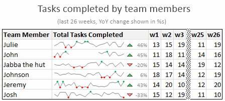
A Sparkline is a small chart that is aligned with rows of some tabular data and usually shows trend information.
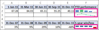
Here is an example of sparklines in a project team status report.
Excel Sparklines Tutorial – 3 steps
Creating sparklines in Excel is very easy. You follow 3 very simple steps to get beautiful sparklines in an instant.
- Select the data from which you want to make a sparkline.
- Go to Insert > Sparkline and select the type of sparkline (you have 3 options – line, column and win-loss chart)
- Specify a target cell where you want the sparkline to be placed
- Optional: Format the sparkline if you want.
Here is a short screen-cast showing you how a sparkline is created.
Types of Sparklines in Excel:
There are 3 basic types of sparklines in Excel 2010. They are,
- Line chart
- Column chart
- Win-loss chart (useful for showing a bunch of wins & losses denoted by 1s and -1s)
Sparkline Formatting and Options – Explored
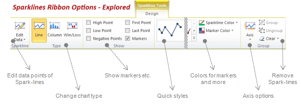
Whenever you select a cell with sparkline in it, you will find a new ribbon called as “Sparklines – Design” ribbon. This is where all the formatting options for sparklines are included. Some of the key formatting / customization options available are,
- Change the sparkline type – between line, column and win/loss
- Change the source data / target cells of sparkline
- Set different colors for first point, last point, highest & lowest points (applicable for column and line chart types)
- Set axis options (show / hide axis, set min and max value for vertical axis, set axis type to date axis etc.)
- Group / un-group a bunch of sparklines (you can change formatting options, axis settings en-masse when you group sparklines)
- Remove sparklines
Sparklines & Missing Data – How does it work?
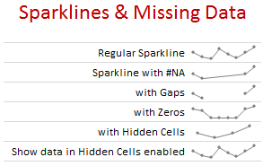
- Non-numeric data: If the sparkline source data contains non-numeric data, they are neglected while plotting the sparklines.
- Errors & #NA values: If data has some #NA values, they are neglected
- Blanks: sparkline show blanks as gaps
- Zeros: If data has zeros, zero value is plotted
- Data in hidden rows / columns: If data has some hidden rows / columns, the values are neglected (unless you enable “Show data in hidden cells” option)
Sparklines in Tables & Pivot Tables
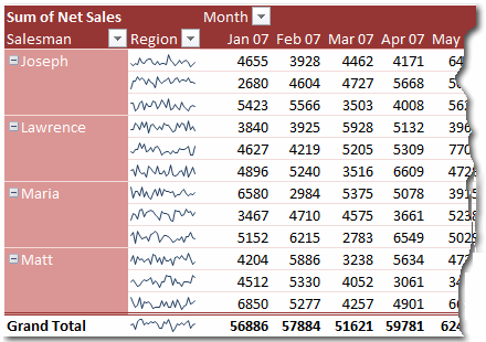
You can add sparklines to tables and pivot tables too. Adding them to pivot tables is a bit tricky but adding sparklines to tables is fairly straightforward and scales nicely.
5 Tips to use Sparklines better
Here is a bunch of quick tips & tricks for those of you starting on sparklines.
- You can auto-fill sparklines. Select the first set of values and add a sparkline. Now copy and past sparklines to auto-fill them based on data in adjacent cells.
- Change their size: When you adjust row-height or column-width of the cell containing sparkline, the size of sparkline changes too.
- Juxtapose sparklines with conditional formatting icons to create stunning charts and dashboards.
- If you want to copy a sparkline over to a ppt or document, you can use “copy as picture” option.
- Enable high / low points to highlight important values
Sparklines & Compatibility
Sparklines are available since Excel 2010. They work in desktop and web versions of Excel.
What happens when someone opens a file with sparklines in Excel 2007?
Sparklines don’t show up in if you open the file in older version of Excel (say Excel 2007).
How does Sparklines compare with other alternatives?
Sparklines vs. In-cell Charts
In-cell charts are a powerful and lightweight way to create bite-sized visualizations. The main technique is to use REPT formula to repetitively show a bunch of symbols (usually | symbol) to create a small chart. The advantage of this approach is that they work in any version of Excel. But the dis-advantage is that we can make only few types of charts (bar charts, column charts by rotating cell text, dot plots). Also, incell charts require some knowledge of excel formulas and creativity.
This is where Excel Sparklines shine, as they are very easy to create and maintain.
Sparklines vs. Conditional Formatting
In Excel 2007, MS introduced a bunch of useful Conditional Formatting options like icons, heat maps that effectively create small visualizations of underlying data. These features are further improved in Excel 2010, 2013 and 2016. While conditional formatting based visualizations are easy to implement and scale very well, there are only few options (a bunch of traffic lights, data bars etc.). This could leave you high and dry if you are looking for rich visualization options. these new features require the actual data to be present in underlying cells (which is a head-ache).
Again, sparklines shine as a simpler and easier alternative.
Sparklines vs. Shrinking an actual chart
We can take an actual chart, strip it of all the clothing (remove gridlines, axis, legend, titles, labels etc.) and resize it so that it fits nicely in a cell [example]. This is the easiest and cleanest way to get sparklines in earlier versions of excel. However this approach has one problem. It doesn’t scale. (ie if you want to get 2 sparklines, you need to do twice the work). Of course, we can write some macros to take care of that, but if you are open to macros, you might as well use SfE and save a lot of trouble. But this approach of shrinking a real chart is better as it gives you full power to customize the underlying chart (add multiple series etc.) which is not available in excel sparklines.
Download Excel Sparklines Tutorial Workbook
Click here to download Excel sparklines tutorial workbook. It shows all three kinds of sparklines in a simple dashboard format. Use the data to create your own sparklines to learn more.
Conclusions on Sparklines
The sparklines in Excel is certainly a great step forward in the world of data visualization. It brings ease and consistency to most users who want better visualizations but do not know how to create them. That said, Microsoft hasn’t really introduced any new types of sparklines since 2010. This is disappointing. Ideally few more types of sparklines such as these can help with dataviz.

On a lighter note, Kudos to Office Team at MS for not adding any 3D capabilities to these sparklines. That would have unleashed a fresh dose of chart monsters.
I use sparklines in most of my dashboards and business reports.
What about you? What are your thoughts on sparklines? Have you used them? What is your experience like? Please share your ideas, impressions and tips thru comments.
Additional examples on Sparklines:


- Sparklines vs. SfE Free Add-in – a detailed comparison [PTS Blog]
- Sparklines for Excel – a fantastic Add-in for generating sparklines in all versions of Excel
Share this tip with your colleagues

Get FREE Excel + Power BI Tips
Simple, fun and useful emails, once per week.
Learn & be awesome.
-
61 Comments -
Ask a question or say something… -
Tagged under
charting, Charts and Graphs, downloads, edward tufte, Excel 2010, excel tables, in-cell charting, Learn Excel, micro charts, Microsoft Excel Conditional Formatting, pivot tables, screencasts, sparklines, tips
-
Category:
Charts and Graphs

Welcome to Chandoo.org
Thank you so much for visiting. My aim is to make you awesome in Excel & Power BI. I do this by sharing videos, tips, examples and downloads on this website. There are more than 1,000 pages with all things Excel, Power BI, Dashboards & VBA here. Go ahead and spend few minutes to be AWESOME.
Read my story • FREE Excel tips book


Excel School made me great at work.
5/5

From simple to complex, there is a formula for every occasion. Check out the list now.

Calendars, invoices, trackers and much more. All free, fun and fantastic.

Power Query, Data model, DAX, Filters, Slicers, Conditional formats and beautiful charts. It’s all here.

Still on fence about Power BI? In this getting started guide, learn what is Power BI, how to get it and how to create your first report from scratch.
Related Tips
61 Responses to “What are Excel Sparklines & How to use them? 5 Secret Tips”
-
 Subhash says:
 Good preview of Sparklines. Will be waiting for your Sparklines for Pivot tables update 🙂
Btw, is it SparkLines, Sparklines or sparklines?
Subhash
-
This is a great new feature in Excel 2010. We are all working with more and more data. As our understanding of the data expands, we need more sophisticated ways to represent trends and patterns in the data. Sometimes basic charts and graphs just don’t show enough information. Because Sparklines offer a way to show a lot of data in a sophisticated, and yet not complicated, visual representation of the data, I think people are really going to use this new feature a lot. And, as you show in this helpful post, it’s pretty easy to create Sparklines with the new Excel. Thanks!
-
Gregor Erbach says:
Too bad I will have to wait for a loooooong time until we get Excel 2010 in my workplace. Maybe I can win a personal licence by writing this comment.
-
This is the first I’ve seen sparklines—thanks for the overview. Can’t wait—this will be powerful! I’m excited to see the capabilities grow for visual analysis!
I’ve built a lot of tools to enable some pretty robust mapping in Google Earth from Excel data. Makes me wonder how future versions of Excel may be able visually represent data not only in charts, but also in maps… Anyone have any thoughts?
-
JeanMarc says:
Hello. I used the SfE add-in to create some dashboards. My colleagues were impressed but the downside is that most people where I work don’t know how to install Excel add-ins, so I’m about the only one to use them. Excel 2010 sparklines really look easy to use. I just hope that we will soon swith to Excel 2010 but knowing of fast our IT moves, I think I’ll have to wait 4-5 years… Thanks.
-
M says:
Cool. Unfortunately, I don’t have Office at home. I wish open office has this feature
-
Hui… says:
Here’s another Quick Tip for Sparklines
===
You can have a sparkline and a number in the same cell
Setup your sparkline as normal, except make the data range 3 or 4 cells longer than you want
If you want a number on the left side insert 3 or 4 =na() in the spare cells to the left of the data
In the sparkline cell type your reference to your data as normal
Good for highlighting the starting or finishing value of the sparkline -
Hui… says:
Here’s another Quick Tip for Sparklines
===
You can also use conditional formatting with sparklines and my previous tip
So a single cell can display 3 pieces of information:
+ a Sparkline,
+ a Value and
+ a Format -
dan l says:
I get some decent mileage out of sparklines as it is. The biggest difficulty is that with SFE is distribution. I hope that excel 2010 solves some of that.
I do wish they’d put some more options in there——for example the only pie chart that I really ever make use of is the SFE pie which is small enough to get a point across effectively yet small enough to not take up a whole page.
Incidentally: if you don’t mind getting a little cute you can do a pretty good impression of the ‘Consumer Reports’ rating system (http://accurateautoadvice.com/images/cr_ratings.jpg) with those little things. It has disadvantages obviously.
Chandoo, the stock chart arrows — in 2010 do you do those with the char map and conditional formatting? Or is that now a built in feature?
-
@Hui.. Excellent tip about using blank cells in the beginning & end to add labels… I didnt know about that.
However, I would not encourage anyone to add all 3 — value, CF and sparkline to same cell, as this could create some really complex visualization and take a ton of time to understand. But it may some interesting applications.
@Dan l … The arrows are part of CF in Excel 2010 (and if I am not wrong, they are in 2007 too).
Reg. your link to consumer report, we have done something similar in excel a while ago — checkout http://chandoo.org/wp/2008/10/07/excel-radar-charts-replacement-spot-matrix-download-template/
@Subash.. I am not sure what it is..
-
Tom says:
Good review — thanks Chandoo!
I like to miniaturize regular charts to allow for the most flexibility. I’ve written a fairly simple macro with automates the process (it places the chart to the right of the data series that I select, and it also links the chart to the cell so that it resizes when the cell is resized). I agree that this new feature will bring the idea to the masses and 1) provide more widespread acceptance and 2) promote more innovation in their implementation.
-
Rob says:
Good overview Chandoo. I look forward to finding a use for these…whenever I can get my hands on Excel 2010.
Rob -
Michael Pennington says:
Great article, as always. I have tried using BonaVista and the free sparklines add in prior to Excel 2010 and find that most of the times when I run into issues—it is related to the scale. Having to load the custom fonts is also problematic (obviously, not in Excel 2010). I believe that the win-loss charts are the sparklines that convey information to the user in the most effective manner. The line and area charts are just too small to convey anything that isn’t an incredibly dramatic shift or very linear info. For example, the monthly net sales by region you show above, looks very good, but it is difficult to glance at and really understand what happened, without going back to the numbers. I am glad they are going more mainstream, I hope to start utilizing them in dashboards more frequently, but as it stands, in-cell charting is still my preferred method. Keep up the great work, Chandoo!
-
Great job as always. You are very thorough and answer all of my questions. I appreciate your posts.
-
dhoff says:
Tom,
Can you share your VBA code to your macro that resizes the chart when the cell is resized?
Thanks!
-
Bruce Spong says:
This is the first I’ve seen sparklines – thanks for the overview. Can’t wait – this is powerful! I’m excited to see the capabilities grow for visual analysis! Makes me look good, too, by adding new features to our dashboards. I look forward to finding a use for these…whenever I can get my hands on Excel 2010~
Cheers~ -
Alexandra says:
I’ve never heard of this before. I’m interested in better ways of presenting data visually, and look forward to trying this out as soon as I get the chance.
-
@Dan l… I am wrong. the up down arrows are new in Excel 2010. In Excel 2007, we can however use font symbols to get similar effect.
@all.. thanks for the comments. I am pretty excited about this new feature too…
-
Squiggler says:
Interesting you can also use Conditional formatting/Sparklines to create progress meters, by simply setting up Min/Value/Max and graphing them using the formatting or sparklines depending on vertical or horizontal orientation. (sparkline has to be one cell, formatting 3 cells) then simply use copy and paste as linked picture, with the sparklines you have to crop out the min and max, I then group the pasted picture with shapes, lines etc to make the chart! which is then re-sizable!
-
Scaffdog845 says:
Sparklines rock! Looks like Microsoft may actually be listening to what the user community needs instead of giving us what they think we need.
-
CMT says:
Thanks, Chandoo!
-
An observation regarding bars/column in the spark line version — in normally sized charts, bars/columns emphasizes individual values because of their visual weight. However, in the spark line version they do not seem to have the same type of weight — look at the table in the post showing the different type of spark lines. While one would normally not use bars to show patterns in the data , in the spark line version I have used them for that purpose. Would be interested to know the experience of other users.
-
jocelyn says:
hello I cant see how to get the graph with the ups/down triangles and percentage changes in sparklines as shown in the first example. How is that done as it looks as if these are in the same cell as the line chart
-
@Jocelyn: I have used conditional formatting icons for that purpose. They are in separate cell. Only that I have removed cell borders and hidden grid lines so that everything looks smooth and merged.
-
jocelyn says:
Thanks for that Chandoo is there any chance to use your as a template as badly need something like yours to work with. If the template had all the formats you had dev it would be great please please
-
Suresh says:
Hi Chandoo,
can u help me in preparation of MIS report of a manufacturing company in MS Excel.
awaiting for ur reply -
Shawn says:
I have Excel 2010 and see the Sparklines module in the ribbon, but it is grayed out, as if it is not enable. Do I require a different version or need to turn the feature on somehow?
-
Hui… says:
@Shawn, Make sure you have selected a number of adjacent cells that are suitable for charting, ie: Numbers only, Don’t include text
-
Did you ever write the post that talked about how to add sparklines in a pivot table?
-
Dann says:
Hi Chandoo, I’m learning a lot, but I can´t practice and bring to life some exaples, specially the ones like this, because I’m using excel 2007, so I would love to win the excel 2010 H&S edition. By the way, your page has helped me a lot at work, reducing for exaple a two days of work in reports to a pair of hours. So my next step, is to create a dashboard integrating all data from every piece of work I have. Thanks!
-
Dave Snyder says:
Great feature — Maybe it’s time to upgrade from MS Office 2003 — long over due.
-
James says:
@Chandoo… Re: June 8, 2010 comment. I am trying to mimic your «smooth and merged» look since users cannot move the icon set to the right of the Sparkline. Since I cannot hide the gridline of just one cell, I colored the left border of the icon set column to white. But I still see the faint, thin white mark at the intersection of each column and row separator. How did you get yours so clean?
-
[…] more information about how to use sparklines, take a look at this blog post. TagsOffice […]
-
Bob C. says:
My son came to me for help with sparkline. I had never used it before but found it very interesting to use. Wish I had seen your explanation of it before experiencing the MS software. We did manage to get through it. By the way it does have 3-D.
-
[…] Debra tells how to setup sparklines for data that is in hidden cells. If you have not tried sparklines, you are missing out on one of the most fun, easy to use charting feature in Excel 2010 / 2013. Check out this tutorial to get started. […]
-
misha says:
Hi, I am not sure how to do it most effectively win pivot when the row vlues change according to slicers
Thanks -
[…] can create this chart very easily with Excel 2010 sparklines. Line chart for productivity and win-loss chart for better or worse […]
-
[…] ????? ?????? ?? ??????? Insert -> Sparklines. ?? ??????? ????? ??? ????? ??? ??????? ???????? […]
-
[…] Some tips samples on how to create and use sparklines in Excel. More samples here. […]
-
[…] Algunos consejos de muestras sobre cómo crear y usar los mini gráficos en Excel. Más ejemplos aquí. […]
-
[…] In Google Spreadsheet you can make them using the =sparkline() formula. In Excel 2010 you can find it in the ribbon. […]
-
sharif says:
when I open excel I do not find the sparklines in the ribbon..! could you inform me how should I add it to the ribbon? on excel 2007
-
Ravi Agrawal says:
Superb Article and explanantions……i will certainly use these sparklines in my dashboards and presentations
-
[…] Learn more about these cool sparklines along with some good tips & tricks for using them. […]
-
Wendy Farkas says:
When you view 2 or 3 lines, you can compare trends (up/down). Don’t you think that when you have a bunch of them, you can’t see the forest for the trees?
In your illustration I see a bunch of lines. I’d be looking for markers or line colors or arrow characters to clue me. Is there such a thing as diminishing returns / too much of a good thing?
-
[…] Sparkline: Is a small chart that is used to identify trends within tables. They are also known as micro charts. You can find more information about sparkline here. […]
-
[…] § Excel 2010 Sparklines Tutorial […]
-
Nicole says:
Pls I need this for college help
-
@Nicole
What is the question?
-
-
[…] Instead of running correlation statistical tests (generating a correlation coefficient), he suggests using visual charts to stack different factors on top of each other, using the same timeline on the x-axis. If you can visually see how variation aligns with other factors, then there might be a correlation. I’ve seen these simplified charts in Excel, called sparklines. Learn more about sparklines >>> […]
-
Maria says:
Great but they cannot be vertical, or am I wrong?
-
Duncan Williamson says:
They can be vertical … if you know how to take a screenshot and crop it. Alternatively, even better, use the camera tool and learn how to swivel!
-
-
vivian.liu says:
I couldn’t find out the add-in Sparklines for Excel in Chinese website, would you pls help share the download link, many thanks.
-
Duncan Williamson says:
I see this page is originally from 2010 but you revived it!
I have done the following with Sparklines, in addition to what you have written:
a very passable Histogram, with no spaces between the columns;
Sparklines with values/text AND up-down arrows and background formatting;
two sets of data, even three and more;
use them together with the camera tool;
scattergraphs;
dynamic horizontal and vertical axesOther odds and ends!
I not really a creative person but Sparklines appeal to me!
-
Prakash says:
Hi Duncan,
Do you have example that you can share in a link? What other resource would you recommend to learn more on what you posted.
Thanks
-
-
Thanks for sharing these links Duncan. Awesome techniques indeed.
-
-
-
-
Thanks for all those informations about Sparklines !!!
-
Karthik says:
Someone plz share Chandoo’s article on «Adding SparkLines inside Pivot».. First time I dont see a hyperlink for something tats interesting in Chandoo’s post 🙂
Leave a Reply
Содержание:
- Что такое спарклайны?
- Типы спарклайнов в Excel
- Вставка спарклайнов в Excel
- Редактирование набора данных существующих спарклайнов
- Работа со скрытыми и пустыми ячейками
- Изменение типа спарклайна
- Выделение точек данных в спарклайнах
- Цвет и стиль спарклайнов
- Добавление оси
- Группировать и разгруппировать спарклайны
- Удаление спарклайнов
Функция спарклайнов была представлена в Excel 2010.
В этой статье вы узнаете все о Excel Sparklines и увидите несколько полезных примеров.
Что такое спарклайны?
Спарклайны — это крошечные диаграммы, которые находятся в ячейке в Excel. Эти диаграммы используются для отображения тенденции во времени или изменения набора данных.
Вы можете использовать эти спарклайны, чтобы улучшить внешний вид ваших мягких данных, добавив этот слой визуального анализа.
Хотя спарклайны представляют собой крошечные диаграммы, они имеют ограниченную функциональность (по сравнению с обычными диаграммами в Excel). Несмотря на это, Sparklines великолепны, так как вы можете создавать их, легко отображая тенденцию (и даже выбросы / максимумы-минимумы) и делать ваши отчеты и панель инструментов более удобными для чтения.
В отличие от обычных диаграмм, спарклайны не являются объектами. Они находятся в ячейке на заднем плане этой ячейки.
Типы спарклайнов в Excel
В Excel существует три типа спарклайнов:
- Линия
- Столбец
- Выигрыш-проигрыш
На изображении ниже я создал пример всех этих трех типов спарклайнов.

Первый в G2 — это спарклайн линейного типа, в G3 — тип столбца, а в G4 — тип выигрыша-проигрыша.
Вот несколько важных вещей, которые нужно знать о Excel Sparklines
- Спарклайны являются динамическими и зависят от базового набора данных. Когда базовый набор данных изменяется, спарклайн обновляется автоматически. Это делает его полезным инструментом при создании панелей мониторинга Excel.
- Размер спарклайнов зависит от размера ячейки. Если вы измените высоту или ширину ячейки, спарклайн изменится соответствующим образом.
- Пока в ячейке есть спарклайн, вы также можете ввести в него текст.
- Вы можете настроить эти спарклайны — например, изменить цвет, добавить ось, выделить максимальные / минимальные точки данных и т. Д. Позже в этом руководстве мы увидим, как это сделать для каждого типа спарклайнов.
Примечание: Спарклайн выигрыша-проигрыша похож на спарклайн столбца, но он не показывает величину значения. Его лучше использовать в ситуациях, когда результат является двоичным, например, Да / Нет, Истина / Ложь, Голова / Хвост, 1 / -1 и т. Д. Например, если вы строите график, шел ли дождь за последние 7 дней или нет, вы можете построить график выигрыша-проигрыша с 1 для дней, когда шел дождь, и с -1 для дней, когда его не было. В этом руководстве все, что описано для спарклайнов столбцов, также можно применить к спарклайнам выигрыша-проигрыша.

Теперь давайте рассмотрим каждый из этих типов спарклайнов и все настройки, которые вы можете с ним сделать.
Вставка спарклайнов в Excel
Допустим, вы хотите вставить спарклайн (как показано ниже).

Вот шаги, чтобы вставить спарклайн в Excel:
- Выберите ячейку, в которой вы хотите создать спарклайн.
- Щелкните вкладку Вставка.

- В группе «Спарклайны» выберите параметр «Линия».
- В диалоговом окне «Создать спарклайны» выберите диапазон данных (в данном примере A2: F2).
- Щелкните ОК.


Это вставит спарклайн в ячейку G2.
Чтобы вставить спарклайн «Столбец» или «Выигрыш-проигрыш», необходимо выполнить те же действия, описанные выше, и выбрать Столбцы или Выигрыш-проигрыш вместо строки (на шаге 3).
Хотя приведенные выше шаги вставляют в ячейку базовый спарклайн, вы можете сделать некоторые настройки, чтобы сделать его лучше.
Выбрав ячейку со спарклайном, вы заметите, что контекстная вкладка — Дизайн инструментов Sparkline — становится доступным. На этой контекстной вкладке вы найдете все параметры настройки для выбранного типа спарклайна.

Редактирование набора данных существующих спарклайнов
Вы можете редактировать данные существующего спарклайна с помощью параметра «Редактировать данные». Когда вы щелкаете раскрывающееся меню «Редактировать данные», вы получаете следующие параметры:
- Изменить местоположение и данные группы: Используйте это, если вы сгруппировали несколько спарклайнов и хотите изменить данные для всей группы (группировка рассматривается позже в этом руководстве).
- Редактировать данные одного спарклайна: Используйте это, чтобы изменить данные только для выбранного спарклайна.

Щелкнув любую из этих опций, вы откроете диалоговое окно «Редактировать спарклайны», в котором вы можете изменить диапазон данных.
Работа со скрытыми и пустыми ячейками
Когда вы создаете линейный спарклайн с набором данных, который имеет пустую ячейку, вы заметите, что спарклайн показывает пробел для этой пустой ячейки.

В приведенном выше наборе данных отсутствует значение апреля, что создает разрыв в первом спарклайне.
Вот пример отсутствия точки данных в спарклайне столбца.

Вы можете указать, как вы хотите обрабатывать эти пустые ячейки.
Вот шаги
- Щелкните ячейку со спарклайном.
- Щелкните вкладку «Дизайн» (контекстная вкладка, которая становится доступной только при выборе ячейки со спарклайном).
- Щелкните параметр «Редактировать данные» (щелкните текстовую часть, а не ее значок).
- В раскрывающемся списке выберите вариант «Скрытые и пустые ячейки».
- В открывшемся диалоговом окне выберите, хотите ли вы отображать
- Пустые ячейки как пробелы
- Пустые ячейки как ноль
- Соедините точки данных до и после линии [этот параметр доступен только для спарклайнов линии].


Если данные для спарклайна находятся в скрытых ячейках, вы можете установить флажок «Показать данные в скрытых строках и столбцах», чтобы убедиться, что данные из этих ячеек также отображаются на графике. Если вы этого не сделаете, данные из скрытых ячеек будут проигнорированы.
Ниже приведен пример всех трех вариантов линейного спарклайна:

- Ячейка G2 — это то, что происходит, когда вы решаете показать зазор в спарклайне.
- Ячейка G3 — это то, что происходит, когда вы выбираете вместо этого показывать ноль.
- Ячейка G2 — это то, что происходит, когда вы выбираете отображение непрерывной линии, соединяя точки данных.
То же самое можно сделать и со спарклайнами столбцов и выигрышей-проигрышей (но не с опцией подключения точек данных).
Изменение типа спарклайна
Если вы хотите быстро изменить тип спарклайна — от строки к столбцу или наоборот, вы можете сделать это, выполнив следующие действия:
- Щелкните спарклайн, который нужно изменить.
- Перейдите на вкладку «Дизайн спарклайнов».
- В группе Тип выберите нужный спарклайн.

Выделение точек данных в спарклайнах
Хотя простой спарклайн показывает тенденцию во времени, вы также можете использовать некоторые маркеры и выделения, чтобы сделать его более значимым.
Например, вы можете выделить максимальную и минимальную точки данных, первую и последнюю точку данных, а также все отрицательные точки данных.
Ниже приведен пример, в котором я выделил максимальную и минимальную точки данных в спарклайне строки и столбца.

Эти параметры доступны на вкладке «Инструменты спарклайна» (в группе «Показать»).

Вот различные доступные варианты:
- Верхняя / нижняя точка: Вы можете использовать любой из них или оба, чтобы выделить максимальную и / или минимальную точку данных.
- Первая / Последняя точка: Вы можете использовать любой из них или оба, чтобы выделить первую и / или последнюю точку данных.
- Отрицательные моменты: Если у вас есть отрицательные значения данных, вы можете использовать эту опцию, чтобы выделить их все сразу.
- Маркеры: Этот параметр доступен только для спарклайнов. Он выделит все точки данных маркером. Вы можете изменить цвет маркера, используя параметр «Цвет маркера».
Цвет и стиль спарклайнов
Вы можете изменить внешний вид спарклайнов, используя параметры стиля и цвета.
Он позволяет изменять цвет спарклайна (линий или столбцов), а также маркеры.

Вы также можете использовать готовые варианты стилей. Чтобы получить полный список опций. щелкните значок раскрывающегося списка в правом нижнем углу поля стиля.

Совет профессионала: Если вы используете маркеры для выделения определенных точек данных, рекомендуется выбрать светлый цвет линии и яркий и темный маркер (в большинстве случаев лучше всего подходит красный).
Добавление оси
Когда вы создаете спарклайн в форме по умолчанию, он показывает самую низкую точку данных внизу, а все остальные точки данных относятся к ней.
В некоторых случаях вы можете не захотеть, чтобы это было так, поскольку кажется, что это показывает огромные различия.
В приведенном ниже примере отклонение составляет всего 5 пунктов (где весь набор данных находится между 95 и 100). Но поскольку ось начинается с самой низкой точки (то есть 95), вариация выглядит огромной.

Эта разница намного более заметна в спарклайне столбца:

В спарклайне столбца выше может показаться, что значение января близко к 0.
Чтобы отрегулировать это, вы можете изменить ось в спарклайнах (сделать так, чтобы она начиналась с определенного значения).
Вот как это сделать
- Выберите ячейку со спарклайном (ами).
- Перейдите на вкладку «Дизайн спарклайновых инструментов».
- Нажмите на опцию Axis.
- В раскрывающемся списке выберите Пользовательское значение (в параметрах минимального значения вертикальной оси).
- В диалоговом окне Параметры вертикальной оси спарклайна введите значение 0.
- Щелкните ОК.


Это даст вам результат, как показано ниже.

Установив таможенную стоимость на 0, мы заставили спарклайн начинать с 0. Это дает истинное представление об изменении.
Примечание. Если в наборе данных есть отрицательные числа, лучше не устанавливать ось. Например, если вы установите для оси значение 0, отрицательные числа не будут отображаться в спарклайне (поскольку он начинается с 0).
Вы также можете сделать ось видимой, выбрав параметр «Показать ось». Это полезно только тогда, когда у вас есть числа, пересекающие ось. Например, если у вас установлена ось на 0 и есть как положительные, так и отрицательные числа, тогда ось будет видна.

Группировать и разгруппировать спарклайны
Если у вас есть несколько спарклайнов в вашем отчете или на панели мониторинга, вы можете сгруппировать некоторые из них вместе. Это позволяет легко вносить изменения во всю группу, а не делать это по одному.
Чтобы сгруппировать спарклайны
- Выберите те, которые хотите сгруппировать.
- Перейдите на вкладку «Дизайн спарклайнов».
- Щелкните значок группы.

Теперь, когда вы выбираете любой из сгруппированных спарклайнов, он автоматически выбирает все из этой группы.
Вы можете разгруппировать эти спарклайны с помощью параметра «Разгруппировать».
Удаление спарклайнов
Вы не можете удалить спарклайн, выбрав ячейку и нажав клавишу удаления.
Чтобы удалить спарклайн, выполните следующие действия:
- Выделите ячейку со спарклайном, который вы хотите удалить.
- Перейдите на вкладку «Дизайн спарклайнов».
- Щелкните опцию Очистить.
