
Содержание
- What Is Short Date In Excel?
- How do I create a short date in Excel?
- What is short date and long date?
- What is short format date?
- What is long date excel?
- How do I convert a short date to a long date in Excel?
- What is a long date format?
- What is Z in date format?
- How do I change a date format from DD MM to yyyy in Excel?
- Which date format is this?
- How do I change a cell to a short date format?
- What date is yyyy-mm-dd?
- How do I use currency 0 in Excel?
- How do you shorten dates?
- What is the long date today?
- What are date functions in Excel?
- Why is Excel showing instead of date?
- Why is my date not formatting in Excel?
- Where is quick analysis tool in Excel?
- What is DDD in date?
- How do you write a long date?
- What is Excel Short Date Format & How to Apply (3 Easy Ways)
- What is Short Date Format in Excel
- How to Apply Short Date Format
- Using Number Format in Ribbon
- Using Format Cells Option
- Using TEXT Function
- Formulas for other short date formats
- How to Change Default Short Date Format
- Short Date Format vs Long Date Format
- Subscribe and be a part of our 15,000+ member family!
What Is Short Date In Excel?
When you type something like 2/2 in a cell, Excel for the web thinks you’re typing a date and shows it as 2-Feb. But you can change the date to be shorter or longer. To see a short date like 2/2/2013, select the cell, and then click Home > Number Format > Short Date.
How do I create a short date in Excel?
Short Date Format in Excel
- Excel provides different ways of displaying dates, be it short date, long date or a customized date.
- Click Home tab, then click the drop-down menu in Number Format Tools.
- Select Short Date from the drop-down list.
- The date is instantly displayed in short date format m/d/yyyy.
What is short date and long date?
Long Date(“D”) Format Specifier. The “D” standard format specifier represents a custom date and time format string defined by the DateTimeFormatInfo. ShortDatePattern property. The custom format string for the Short Date Format Specifier is “dddd , dd MMMM yyyy”.
What is short format date?
Short format: dd/MM/yy (Example: 13/06/03) Medium format: dd/MM/yyyy (Example: 13/06/2003) Long format: d’ de ‘MMMM’ de ‘yyyy (Example: 13 de junio de 2003)
What is long date excel?
The long date option adds the day of the week and writes out the month. So 1/1/19 will display as Tuesday, January 1, 2019. The date will display in the format you choose, no matter how you enter it. If you type “1/1/19” into a cell with the long date format, Excel will change it to the expanded date.
How do I convert a short date to a long date in Excel?
To quickly change date format in Excel to the default formatting, do the following:
- Select the dates you want to format.
- On the Home tab, in the Number group, click the little arrow next to the Number Format box, and select the desired format – short date, long date or time.
What is a long date format?
Long Date. Displays only date values, as specified by the Long Date format in your Windows regional settings. Monday, August 27, 2018. Medium Date. Displays the date as dd/mmm/yy, but uses the date separator specified in your Windows regional settings.
What is Z in date format?
Z is the zone designator for the zero UTC offset. “09:30 UTC” is therefore represented as “09:30Z” or “T0930Z”. “14:45:15 UTC” would be “14:45:15Z” or “T144515Z”. The Z suffix in the ISO 8601 time representation is sometimes referred to as “Zulu time” because the same letter is used to designate the Zulu time zone.
How do I change a date format from DD MM to yyyy in Excel?
To change the date display in Excel follow these steps:
- Go to Format Cells > Custom.
- Enter dd/mm/yyyy in the available space.
Which date format is this?
Date Format Types
| Format | Date order | Description |
|---|---|---|
| 1 | MM/DD/YY | Month-Day-Year with leading zeros (02/17/2009) |
| 2 | DD/MM/YY | Day-Month-Year with leading zeros (17/02/2009) |
| 3 | YY/MM/DD | Year-Month-Day with leading zeros (2009/02/17) |
| 4 | Month D, Yr | Month name-Day-Year with no leading zeros (February 17, 2009) |
How do I change a cell to a short date format?
Follow these steps:
- Select the cells you want to format.
- Press CTRL+1.
- In the Format Cells box, click the Number tab.
- In the Category list, click Date.
- Under Type, pick a date format.
- If you want to use a date format according to how another language displays dates, choose the language in Locale (location).
What date is yyyy-mm-dd?
| Format | Description |
|---|---|
| MM/DD/YY | Two-digit month, separator, two-digit day, separator, last two digits of year (example: 12/15/99) |
| YYYY/MM/DD | Four-digit year, separator, two-digit month, separator, two-digit day (example: 1999/12/15) |
How do I use currency 0 in Excel?
Format numbers as currency in Excel for the web
- Select the cells that you want to format and then, in the Number group on the Home tab, click the down arrow in the Number Format box.
- Choose either Currency or Accounting.
How do you shorten dates?
16. How dates are written and abbreviated
- In most countries of the world, dates are written in order DAY/MONTH/YEAR, e.g., 4 July 1999, abbreviated 4/7/1999.
- In eastern Asia, however, dates are written in order YEAR/MONTH/DAY: 1999 July 4, abbreviated 1999/7/4.
What is the long date today?
| Today’s Date in Other Date Formats | |
|---|---|
| Unix Epoch: | 1639391773 |
| RFC 2822: | Mon, 13 Dec 2021 02:36:13 -0800 |
| DD-MM-YYYY: | 13-12-2021 |
| MM-DD-YYYY: | 12-13-2021 |
What are date functions in Excel?
The DATE function is an Excel function that combines three separate values (year, month, and day) to form a date. When used along with other Excel functions, it can be used to perform a wide range of tasks related to dates, including returning specified dates.
Why is Excel showing instead of date?
Microsoft Excel might show ##### in cells when a column isn’t wide enough to show all of the cell contents. Formulas that return dates and times as negative values can also show as #####.If dates are too long, click Home > arrow next to Number Format, and pick Short Date.
Why is my date not formatting in Excel?
If you want to sort the dates, or change their format, you’ll have to convert them to numbers – that’s how Excel stores valid dates. Sometimes, you can fix the dates by copying a blank cell, then selecting the date cells, and using Paste Special > Add to change them to real dates.
Whenever you select a cell range, the Quick Analysis button will appear in the lower-right corner of the selection. When you click it, you’ll be able to choose from a variety of charts, sparklines, conditional formatting options, and more.
What is DDD in date?
The “ddd” custom format specifier represents the abbreviated name of the day of the week. The localized abbreviated name of the day of the week is retrieved from the DateTimeFormatInfo. AbbreviatedDayNames property of the current or specified culture.
How do you write a long date?
Sometimes, a date is written in long form, like this: Sunday, June 28, 2015 (note that there are commas after the day of the week and the day of the month, but there is no comma after the month). Sometimes, a date is written in numerical form, like this: 6/28/15 or 6/28/2015 (month/date/year).
Источник
What is Excel Short Date Format & How to Apply (3 Easy Ways)
This probably never dragged too much attention because it was always there but all of a sudden you’re finding that taken-for-granted Short Date because you’ve been handed down Long Dates that contain too much information on the whole. With your worksheet bustling and your columns many in number, a Short Date format can be a needed input.
In this tutorial, you’ll find the difference between Short and Long Date formats, how to change the default Short Date format, and 3 easy ways to apply a Short Date format with Number Format on the Ribbon, Format Cells, and the TEXT function.
And first, what is the Short Date format?

Table of Contents
What is Short Date Format in Excel
Enter the date 1-31-25 on the worksheet. The cell will snap to a date format and the entered date will snap to 1/31/2025. This Excel folk is a Short Date format and will include the shorter sides of the day, month, and year combination.
The above-mentioned format is the default, depends on the Regional format set in your computer’s Time and Language settings, English (United States) in our case. Therefore, the default format can be changed using the same settings.
With English (United States), the date components can be slightly different in other Short Date formats. The day in the Short Date format will be displayed in a single digit (1 to 31) or double digits (01 to 31). The month can be single or double digits or a 3-letter abbreviation of the month name. The year can be in double digits or in full. Any combination of these makes up a Short Date.
Short Date formats steers clear of the full month name, day name, and time which can be part of a Long Date. Other Short Date formats, with English (United States) as your computer’s Regional format setting, are listed below. All the dates are Short Date formats of the date 1 st of February 2025:
Computer’s Regional format: English (United States)
| Short Date | Format | Comments |
|---|---|---|
| 1/31/2025 | m/d/yyyy | Default format |
| 2/1/25 | m/d/yy | Other formats |
| 02/01/25 | mm/dd/yy | |
| 02/01/2025 | mm/dd/yyyy | |
| 25/02/01 | yy/mm/dd | |
| 2025-02-01 | yyyy-mm-dd | |
| 01-Feb-25 | dd-mmm-yy |
Do you want know how to apply any of them?
Let’s get formatting!
How to Apply Short Date Format
If you’re at the point of data entry, all you have to do is enter the date in one of the acceptable formats and you will get a Short Date in return.
The format that the date is returned in depends on the system settings of the Regional format; English (United States) in our case. See what type of date you need to enter and the type of Short Date Excel will return:
| Date entered | Date returned |
|---|---|
| 1/31/25 | 1/31/2025 |
| 1-31-25 | 1/31/2025 |
| 2025-1-31 | 1/31/2025 |
| 31 jan 25 | 31-Jan-25 |
The returned Short Date formats are:
Depending on how the date is entered, one of two formats will be returned. When the month is entered numerically, the default Short Date format is returned i.e. m/d/yyyy. Since the default format has the month mentioned first, enter the dates month-first for them to be accepted by Excel.
When the month is entered alphabetically, the date is returned in this d/mmm/yy format with the month name abbreviated.
That’s how to deal with Short Dates when you’re creating your dataset. There’s equally the possibility that you’re dealing with ready data that has dates a mile long. There are a few quick ways you can tackle changing Long Dates to Short Dates or even if you want to change the Short Date from one format to another.
Let’s dive into the methods of applying the Short Date format to dates in Excel.
Using Number Format in Ribbon
This method applies the default Short Date format to the selected dates. Since dates are entered in the default Short Date format, the Ribbon option only concerns dates that are in a different format; whether Long or Custom.
Let’s see to this with an example we have set up with the order and delivery dates regarding the product deliveries scheduled for a slot of 6 days. For the dispatch department, the Long Date format makes more sense with the day and time mentioned. But for other departments, where reports may be drafted with many columns, we’ll try to condense the date as much as possible and that calls for the Short Date format.
To bring your dates back to the default Short Date format, use the Number Format Bar in the Ribbon with these steps:
- Select the dates that you want in the default Short Date
- Click on the Number Format Bar‘s arrow to view the Number Format menu in the Home tab’s Number

- Select the Short Date option from the menu.

And that click will switch the format of the selected dates to the default Short Date format:

Notes:
Select any date from the Short Dates and note in the Formula Bar that the actual value of the cell doesn’t change with a change in format, only the display.
The Number Format Bar will display Date as the format when the selected cell is formatted to the default Short or Long Date format.
For the formatting to work, the cell must carry a date value (which can be deduced also from the alignment to the right). If the date is copied or entered as text, Number Formats will make no changes to them.
Using Format Cells Option
You’re likely to resort to this option when you want a Short Date format but not Excel’s default one. Format Cells gives you various options for Short Date formats and also room for custom formats. This way, you can modify the placement of the date components and even add your choice of separators.
Let’s cut some dates short. Use the Format Cells option to apply a Short Date format in Excel with the following steps:
- Select the cells containing the dates you want to reformat.
- From the Ribbon, select the dialog launcher of the Home tab’s Number group to access the Format Cells dialog box.
- Using the Number group’s launcher opens the Format Cells dialog box in the Number tab directly.

- In the dialog box, go through the format types in the Date category to choose a Short Date format of preference.

If you’ve found what you want, use the OK button to apply it but would this even be a neat tutorial without giving you more ideas?
At this point, you can use the Locale (location) to get a location-specific format which may include the locale’s native language in the date.
We talked about custom formats earlier and now would be the best time to collate one by heading to the Custom category. Before that, picking a format from the Date category first will allow you to edit that format in the Custom category.
- Go to the Custom category and it will carry the formatting code of the format selected in the Date

- Use the code as a base to edit it into a custom code for a CustomShort Date
- We will change the separator from a hyphen to a period and change the day component from «d» to «dd» so that the day will be displayed in double digits instead of a single digit. 1 will be displayed as 01; look at the Sample box before and after editing the code to see a preview of this change.

- Hit the OK command in the dialog box.
The dates will now have a custom Short Date format, also confirmed by the Number Format Bar:

That’s the good thing about formatting; the dates will be usable in calculations and date formulas. When it won’t be a good thing is the case of wanting to use the date as text. This is Excel so a lot of these notions should be possible, right? This innocent notion can come true thanks to the TEXT function so read up ahead!
Using TEXT Function
The TEXT function can return the date as a Short Date in text format. The date needs to be the only value present in the cell so that the function knows what to pick on. The TEXT function converts the cell value to text in the supplied format. We will feed the TEXT function with our choice of Short Date format so it can return the Long Dates as Short Dates in text form.
Dates won’t always need to be used in calculations and you may need the date to be a part of a text to go on a receipt, footnote, or email message for example. There was also something we said about rearranging the components of the date so let’s see what the TEXT function can do for us. Enter the formula below to use the TEXT function to apply a Short Date format:
Columns C and D in our case example have the original Long Dates. Taking the first date in C3, we’ve applied the format «m/d/yyyy» with the year component placed first, enclosed in double quotes. All the rest of the Long Dates in the dataset also follow:

The Number Format Bar also shows that the resulting value is not in a date format anymore. Now you can pick the text from here and place it as text wherever needed.
Formulas for other short date formats
It’s not just the default Short Date format that the TEXT function will be able to work with. You can go with any other Short Date format of preference or the format that conforms to the default Short Date format as per your computer’s Regional format settings. Enter the relevant Short Date format in the formula such as:
See how this would apply to a Long Date:

If you’re going totally unconventional, the TEXT function can accept that too like this formula below:
This Short Date format has the date components regrouped and separated with the vertical bar. Here’s how it worked out in Excel:

How to Change Default Short Date Format
By now, we’re well familiar that the default Short Date format is m/d/yyyy. This format being the default is resultant of the Regional format set as English (United States). The format may change by changing this setting but you can also change the default Short Date format leaving the Regional format untouched. Either way, these are the steps to go about if you want to change the default Short Date format:
- Visit the Start Menu of your computer and select the Settings
- Select Time & Language on the Settings

- Now select the Region tab from the pane on the left.
This is the part you’re interested in when it comes to some default settings of your computer such as the Short and Long Date and time formats, the region, the first day of the week, etc.
If you change the region in the Regional format setting, this may also automatically change the default Short Date format e.g. the default format for a Short Date with English (United Kingdom) as the Regional format is dd/mm/yyyy.
But keeping the Regional format constant, you can still change the default Short Date format and for that, proceed with these steps:
- At the bottom of the Region settings click on the last option reading Change data formats.

- Click on the arrow of the Short Date bar and select a different format for the default Short Date.

Regional format data will instantly be updated.

Now when a date is entered in Excel, the new default format for the Short Date will be applied and you can confirm this change from the Number Format Bar which shows the updated default Short Date format:

Short Date Format vs Long Date Format
The Short Date format does not include the full month name, only the 3-letter abbreviation at most. By default, the representation of the month component is numerical. The Long Date format displays the complete month name and may show the day name and time.
The Short Date format is applied by default to dates whereas the Long Date format is applied by the user. A Short Date entered that takes on the default format will be a date value that can be used in calculations and date functions.
The Short Date format has the date components divided by a separator (forward slash or hyphen mostly) after the first and second components in the date. The Long Date format includes commas as the separator by default.
Use the Short Date format to quickly enter the date and also where you would prefer to have compact dates and narrow columns. Use the Long Date format to feature the day, full month, or time for quick analysis.
To sum it up shortly, the Short Date format is applied by default to a date entered in Excel. It can be customized to be displayed differently and can be converted to text and is space efficient. While you’re chipping at your Excel Long Dates to shorten them, we’ll come up with more Excel chiseling, hacking away at another problem!
Subscribe and be a part of our 15,000+ member family!
Now subscribe to Excel Trick and get a free copy of our ebook «200+ Excel Shortcuts» (printable format) to catapult your productivity.
Источник
Many users find that using an external keyboard with keyboard shortcuts for Excel helps them work more efficiently. For users with mobility or vision disabilities, keyboard shortcuts can be easier than using the touchscreen and are an essential alternative to using a mouse.
Notes:
-
The shortcuts in this topic refer to the US keyboard layout. Keys for other layouts might not correspond exactly to the keys on a US keyboard.
-
A plus sign (+) in a shortcut means that you need to press multiple keys at the same time.
-
A comma sign (,) in a shortcut means that you need to press multiple keys in order.
This article describes the keyboard shortcuts, function keys, and some other common shortcut keys in Excel for Windows.
Notes:
-
To quickly find a shortcut in this article, you can use the Search. Press Ctrl+F, and then type your search words.
-
If an action that you use often does not have a shortcut key, you can record a macro to create one. For instructions, go to Automate tasks with the Macro Recorder.
-
Download our 50 time-saving Excel shortcuts quick tips guide.
-
Get the Excel 2016 keyboard shortcuts in a Word document: Excel keyboard shortcuts and function keys.
In this topic
-
Frequently used shortcuts
-
Ribbon keyboard shortcuts
-
Use the Access keys for ribbon tabs
-
Work in the ribbon with the keyboard
-
-
Keyboard shortcuts for navigating in cells
-
Keyboard shortcuts for formatting cells
-
Keyboard shortcuts in the Paste Special dialog box in Excel 2013
-
-
Keyboard shortcuts for making selections and performing actions
-
Keyboard shortcuts for working with data, functions, and the formula bar
-
Keyboard shortcuts for refreshing external data
-
Power Pivot keyboard shortcuts
-
Function keys
-
Other useful shortcut keys
Frequently used shortcuts
This table lists the most frequently used shortcuts in Excel.
|
To do this |
Press |
|---|---|
|
Close a workbook. |
Ctrl+W |
|
Open a workbook. |
Ctrl+O |
|
Go to the Home tab. |
Alt+H |
|
Save a workbook. |
Ctrl+S |
|
Copy selection. |
Ctrl+C |
|
Paste selection. |
Ctrl+V |
|
Undo recent action. |
Ctrl+Z |
|
Remove cell contents. |
Delete |
|
Choose a fill color. |
Alt+H, H |
|
Cut selection. |
Ctrl+X |
|
Go to the Insert tab. |
Alt+N |
|
Apply bold formatting. |
Ctrl+B |
|
Center align cell contents. |
Alt+H, A, C |
|
Go to the Page Layout tab. |
Alt+P |
|
Go to the Data tab. |
Alt+A |
|
Go to the View tab. |
Alt+W |
|
Open the context menu. |
Shift+F10 or Windows Menu key |
|
Add borders. |
Alt+H, B |
|
Delete column. |
Alt+H, D, C |
|
Go to the Formula tab. |
Alt+M |
|
Hide the selected rows. |
Ctrl+9 |
|
Hide the selected columns. |
Ctrl+0 |
Top of Page
Ribbon keyboard shortcuts
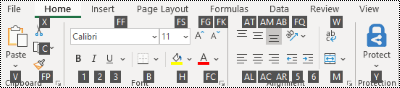
The ribbon groups related options on tabs. For example, on the Home tab, the Number group includes the Number Format option. Press the Alt key to display the ribbon shortcuts, called Key Tips, as letters in small images next to the tabs and options as shown in the image below.
You can combine the Key Tips letters with the Alt key to make shortcuts called Access Keys for the ribbon options. For example, press Alt+H to open the Home tab, and Alt+Q to move to the Tell me or Search field. Press Alt again to see KeyTips for the options for the selected tab.
Depending on the version of Microsoft 365 you are using, the Search text field at the top of the app window might be called Tell Me instead. Both offer a largely similar experience, but some options and search results can vary.
In Office 2013 and Office 2010, most of the old Alt key menu shortcuts still work, too. However, you need to know the full shortcut. For example, press Alt, and then press one of the old menu keys, for example, E (Edit), V (View), I (Insert), and so on. A notification pops up saying you’re using an access key from an earlier version of Microsoft 365. If you know the entire key sequence, go ahead, and use it. If you don’t know the sequence, press Esc and use Key Tips instead.
Use the Access keys for ribbon tabs
To go directly to a tab on the ribbon, press one of the following access keys. Additional tabs might appear depending on your selection in the worksheet.
|
To do this |
Press |
|---|---|
|
Move to the Tell me or Search field on the ribbon and type a search term for assistance or Help content. |
Alt+Q, then enter the search term. |
|
Open the File menu. |
Alt+F |
|
Open the Home tab and format text and numbers and use the Find tool. |
Alt+H |
|
Open the Insert tab and insert PivotTables, charts, add-ins, Sparklines, pictures, shapes, headers, or text boxes. |
Alt+N |
|
Open the Page Layout tab and work with themes, page setup, scale, and alignment. |
Alt+P |
|
Open the Formulas tab and insert, trace, and customize functions and calculations. |
Alt+M |
|
Open the Data tab and connect to, sort, filter, analyze, and work with data. |
Alt+A |
|
Open the Review tab and check spelling, add notes and threaded comments, and protect sheets and workbooks. |
Alt+R |
|
Open the View tab and preview page breaks and layouts, show and hide gridlines and headings, set zoom magnification, manage windows and panes, and view macros. |
Alt+W |
Top of Page
Work in the ribbon with the keyboard
|
To do this |
Press |
|---|---|
|
Select the active tab on the ribbon and activate the access keys. |
Alt or F10. To move to a different tab, use access keys or the arrow keys. |
|
Move the focus to commands on the ribbon. |
Tab key or Shift+Tab |
|
Move down, up, left, or right, respectively, among the items on the ribbon. |
Arrow keys |
|
Show the tooltip for the ribbon element currently in focus. |
Ctrl+Shift+F10 |
|
Activate a selected button. |
Spacebar or Enter |
|
Open the list for a selected command. |
Down arrow key |
|
Open the menu for a selected button. |
Alt+Down arrow key |
|
When a menu or submenu is open, move to the next command. |
Down arrow key |
|
Expand or collapse the ribbon. |
Ctrl+F1 |
|
Open a context menu. |
Shift+F10 Or, on a Windows keyboard, the Windows Menu key (usually between the Alt Gr and right Ctrl keys) |
|
Move to the submenu when a main menu is open or selected. |
Left arrow key |
|
Move from one group of controls to another. |
Ctrl+Left or Right arrow key |
Top of Page
Keyboard shortcuts for navigating in cells
|
To do this |
Press |
|---|---|
|
Move to the previous cell in a worksheet or the previous option in a dialog box. |
Shift+Tab |
|
Move one cell up in a worksheet. |
Up arrow key |
|
Move one cell down in a worksheet. |
Down arrow key |
|
Move one cell left in a worksheet. |
Left arrow key |
|
Move one cell right in a worksheet. |
Right arrow key |
|
Move to the edge of the current data region in a worksheet. |
Ctrl+Arrow key |
|
Enter the End mode, move to the next nonblank cell in the same column or row as the active cell, and turn off End mode. If the cells are blank, move to the last cell in the row or column. |
End, Arrow key |
|
Move to the last cell on a worksheet, to the lowest used row of the rightmost used column. |
Ctrl+End |
|
Extend the selection of cells to the last used cell on the worksheet (lower-right corner). |
Ctrl+Shift+End |
|
Move to the cell in the upper-left corner of the window when Scroll lock is turned on. |
Home+Scroll lock |
|
Move to the beginning of a worksheet. |
Ctrl+Home |
|
Move one screen down in a worksheet. |
Page down |
|
Move to the next sheet in a workbook. |
Ctrl+Page down |
|
Move one screen to the right in a worksheet. |
Alt+Page down |
|
Move one screen up in a worksheet. |
Page up |
|
Move one screen to the left in a worksheet. |
Alt+Page up |
|
Move to the previous sheet in a workbook. |
Ctrl+Page up |
|
Move one cell to the right in a worksheet. Or, in a protected worksheet, move between unlocked cells. |
Tab key |
|
Open the list of validation choices on a cell that has data validation option applied to it. |
Alt+Down arrow key |
|
Cycle through floating shapes, such as text boxes or images. |
Ctrl+Alt+5, then the Tab key repeatedly |
|
Exit the floating shape navigation and return to the normal navigation. |
Esc |
|
Scroll horizontally. |
Ctrl+Shift, then scroll your mouse wheel up to go left, down to go right |
|
Zoom in. |
Ctrl+Alt+Equal sign ( = ) |
|
Zoom out. |
Ctrl+Alt+Minus sign (-) |
Top of Page
Keyboard shortcuts for formatting cells
|
To do this |
Press |
|---|---|
|
Open the Format Cells dialog box. |
Ctrl+1 |
|
Format fonts in the Format Cells dialog box. |
Ctrl+Shift+F or Ctrl+Shift+P |
|
Edit the active cell and put the insertion point at the end of its contents. Or, if editing is turned off for the cell, move the insertion point into the formula bar. If editing a formula, toggle Point mode off or on so you can use the arrow keys to create a reference. |
F2 |
|
Insert a note. Open and edit a cell note. |
Shift+F2 Shift+F2 |
|
Insert a threaded comment. Open and reply to a threaded comment. |
Ctrl+Shift+F2 Ctrl+Shift+F2 |
|
Open the Insert dialog box to insert blank cells. |
Ctrl+Shift+Plus sign (+) |
|
Open the Delete dialog box to delete selected cells. |
Ctrl+Minus sign (-) |
|
Enter the current time. |
Ctrl+Shift+Colon (:) |
|
Enter the current date. |
Ctrl+Semicolon (;) |
|
Switch between displaying cell values or formulas in the worksheet. |
Ctrl+Grave accent (`) |
|
Copy a formula from the cell above the active cell into the cell or the formula bar. |
Ctrl+Apostrophe (‘) |
|
Move the selected cells. |
Ctrl+X |
|
Copy the selected cells. |
Ctrl+C |
|
Paste content at the insertion point, replacing any selection. |
Ctrl+V |
|
Open the Paste Special dialog box. |
Ctrl+Alt+V |
|
Italicize text or remove italic formatting. |
Ctrl+I or Ctrl+3 |
|
Bold text or remove bold formatting. |
Ctrl+B or Ctrl+2 |
|
Underline text or remove underline. |
Ctrl+U or Ctrl+4 |
|
Apply or remove strikethrough formatting. |
Ctrl+5 |
|
Switch between hiding objects, displaying objects, and displaying placeholders for objects. |
Ctrl+6 |
|
Apply an outline border to the selected cells. |
Ctrl+Shift+Ampersand sign (&) |
|
Remove the outline border from the selected cells. |
Ctrl+Shift+Underscore (_) |
|
Display or hide the outline symbols. |
Ctrl+8 |
|
Use the Fill Down command to copy the contents and format of the topmost cell of a selected range into the cells below. |
Ctrl+D |
|
Apply the General number format. |
Ctrl+Shift+Tilde sign (~) |
|
Apply the Currency format with two decimal places (negative numbers in parentheses). |
Ctrl+Shift+Dollar sign ($) |
|
Apply the Percentage format with no decimal places. |
Ctrl+Shift+Percent sign (%) |
|
Apply the Scientific number format with two decimal places. |
Ctrl+Shift+Caret sign (^) |
|
Apply the Date format with the day, month, and year. |
Ctrl+Shift+Number sign (#) |
|
Apply the Time format with the hour and minute, and AM or PM. |
Ctrl+Shift+At sign (@) |
|
Apply the Number format with two decimal places, thousands separator, and minus sign (-) for negative values. |
Ctrl+Shift+Exclamation point (!) |
|
Open the Insert hyperlink dialog box. |
Ctrl+K |
|
Check spelling in the active worksheet or selected range. |
F7 |
|
Display the Quick Analysis options for selected cells that contain data. |
Ctrl+Q |
|
Display the Create Table dialog box. |
Ctrl+L or Ctrl+T |
|
Open the Workbook Statistics dialog box. |
Ctrl+Shift+G |
Top of Page
Keyboard shortcuts in the Paste Special dialog box in Excel 2013
In Excel 2013, you can paste a specific aspect of the copied data like its formatting or value using the Paste Special options. After you’ve copied the data, press Ctrl+Alt+V, or Alt+E+S to open the Paste Special dialog box.
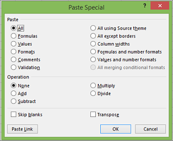
Tip: You can also select Home > Paste > Paste Special.
To pick an option in the dialog box, press the underlined letter for that option. For example, press the letter C to pick the Comments option.
|
To do this |
Press |
|---|---|
|
Paste all cell contents and formatting. |
A |
|
Paste only the formulas as entered in the formula bar. |
F |
|
Paste only the values (not the formulas). |
V |
|
Paste only the copied formatting. |
T |
|
Paste only comments and notes attached to the cell. |
C |
|
Paste only the data validation settings from copied cells. |
N |
|
Paste all cell contents and formatting from copied cells. |
H |
|
Paste all cell contents without borders. |
X |
|
Paste only column widths from copied cells. |
W |
|
Paste only formulas and number formats from copied cells. |
R |
|
Paste only the values (not formulas) and number formats from copied cells. |
U |
Top of Page
Keyboard shortcuts for making selections and performing actions
|
To do this |
Press |
|---|---|
|
Select the entire worksheet. |
Ctrl+A or Ctrl+Shift+Spacebar |
|
Select the current and next sheet in a workbook. |
Ctrl+Shift+Page down |
|
Select the current and previous sheet in a workbook. |
Ctrl+Shift+Page up |
|
Extend the selection of cells by one cell. |
Shift+Arrow key |
|
Extend the selection of cells to the last nonblank cell in the same column or row as the active cell, or if the next cell is blank, to the next nonblank cell. |
Ctrl+Shift+Arrow key |
|
Turn extend mode on and use the arrow keys to extend a selection. Press again to turn off. |
F8 |
|
Add a non-adjacent cell or range to a selection of cells by using the arrow keys. |
Shift+F8 |
|
Start a new line in the same cell. |
Alt+Enter |
|
Fill the selected cell range with the current entry. |
Ctrl+Enter |
|
Complete a cell entry and select the cell above. |
Shift+Enter |
|
Select an entire column in a worksheet. |
Ctrl+Spacebar |
|
Select an entire row in a worksheet. |
Shift+Spacebar |
|
Select all objects on a worksheet when an object is selected. |
Ctrl+Shift+Spacebar |
|
Extend the selection of cells to the beginning of the worksheet. |
Ctrl+Shift+Home |
|
Select the current region if the worksheet contains data. Press a second time to select the current region and its summary rows. Press a third time to select the entire worksheet. |
Ctrl+A or Ctrl+Shift+Spacebar |
|
Select the current region around the active cell. |
Ctrl+Shift+Asterisk sign (*) |
|
Select the first command on the menu when a menu or submenu is visible. |
Home |
|
Repeat the last command or action, if possible. |
Ctrl+Y |
|
Undo the last action. |
Ctrl+Z |
|
Expand grouped rows or columns. |
While hovering over the collapsed items, press and hold the Shift key and scroll down. |
|
Collapse grouped rows or columns. |
While hovering over the expanded items, press and hold the Shift key and scroll up. |
Top of Page
Keyboard shortcuts for working with data, functions, and the formula bar
|
To do this |
Press |
|---|---|
|
Turn on or off tooltips for checking formulas directly in the formula bar or in the cell you’re editing. |
Ctrl+Alt+P |
|
Edit the active cell and put the insertion point at the end of its contents. Or, if editing is turned off for the cell, move the insertion point into the formula bar. If editing a formula, toggle Point mode off or on so you can use the arrow keys to create a reference. |
F2 |
|
Expand or collapse the formula bar. |
Ctrl+Shift+U |
|
Cancel an entry in the cell or formula bar. |
Esc |
|
Complete an entry in the formula bar and select the cell below. |
Enter |
|
Move the cursor to the end of the text when in the formula bar. |
Ctrl+End |
|
Select all text in the formula bar from the cursor position to the end. |
Ctrl+Shift+End |
|
Calculate all worksheets in all open workbooks. |
F9 |
|
Calculate the active worksheet. |
Shift+F9 |
|
Calculate all worksheets in all open workbooks, regardless of whether they have changed since the last calculation. |
Ctrl+Alt+F9 |
|
Check dependent formulas, and then calculate all cells in all open workbooks, including cells not marked as needing to be calculated. |
Ctrl+Alt+Shift+F9 |
|
Display the menu or message for an Error Checking button. |
Alt+Shift+F10 |
|
Display the Function Arguments dialog box when the insertion point is to the right of a function name in a formula. |
Ctrl+A |
|
Insert argument names and parentheses when the insertion point is to the right of a function name in a formula. |
Ctrl+Shift+A |
|
Insert the AutoSum formula |
Alt+Equal sign ( = ) |
|
Invoke Flash Fill to automatically recognize patterns in adjacent columns and fill the current column |
Ctrl+E |
|
Cycle through all combinations of absolute and relative references in a formula if a cell reference or range is selected. |
F4 |
|
Insert a function. |
Shift+F3 |
|
Copy the value from the cell above the active cell into the cell or the formula bar. |
Ctrl+Shift+Straight quotation mark («) |
|
Create an embedded chart of the data in the current range. |
Alt+F1 |
|
Create a chart of the data in the current range in a separate Chart sheet. |
F11 |
|
Define a name to use in references. |
Alt+M, M, D |
|
Paste a name from the Paste Name dialog box (if names have been defined in the workbook). |
F3 |
|
Move to the first field in the next record of a data form. |
Enter |
|
Create, run, edit, or delete a macro. |
Alt+F8 |
|
Open the Microsoft Visual Basic For Applications Editor. |
Alt+F11 |
|
Open the Power Query Editor |
Alt+F12 |
Top of Page
Keyboard shortcuts for refreshing external data
Use the following keys to refresh data from external data sources.
|
To do this |
Press |
|---|---|
|
Stop a refresh operation. |
Esc |
|
Refresh data in the current worksheet. |
Ctrl+F5 |
|
Refresh all data in the workbook. |
Ctrl+Alt+F5 |
Top of Page
Power Pivot keyboard shortcuts
Use the following keyboard shortcuts with Power Pivot in Microsoft 365, Excel 2019, Excel 2016, and Excel 2013.
|
To do this |
Press |
|---|---|
|
Open the context menu for the selected cell, column, or row. |
Shift+F10 |
|
Select the entire table. |
Ctrl+A |
|
Copy selected data. |
Ctrl+C |
|
Delete the table. |
Ctrl+D |
|
Move the table. |
Ctrl+M |
|
Rename the table. |
Ctrl+R |
|
Save the file. |
Ctrl+S |
|
Redo the last action. |
Ctrl+Y |
|
Undo the last action. |
Ctrl+Z |
|
Select the current column. |
Ctrl+Spacebar |
|
Select the current row. |
Shift+Spacebar |
|
Select all cells from the current location to the last cell of the column. |
Shift+Page down |
|
Select all cells from the current location to the first cell of the column. |
Shift+Page up |
|
Select all cells from the current location to the last cell of the row. |
Shift+End |
|
Select all cells from the current location to the first cell of the row. |
Shift+Home |
|
Move to the previous table. |
Ctrl+Page up |
|
Move to the next table. |
Ctrl+Page down |
|
Move to the first cell in the upper-left corner of selected table. |
Ctrl+Home |
|
Move to the last cell in the lower-right corner of selected table. |
Ctrl+End |
|
Move to the first cell of the selected row. |
Ctrl+Left arrow key |
|
Move to the last cell of the selected row. |
Ctrl+Right arrow key |
|
Move to the first cell of the selected column. |
Ctrl+Up arrow key |
|
Move to the last cell of selected column. |
Ctrl+Down arrow key |
|
Close a dialog box or cancel a process, such as a paste operation. |
Ctrl+Esc |
|
Open the AutoFilter Menu dialog box. |
Alt+Down arrow key |
|
Open the Go To dialog box. |
F5 |
|
Recalculate all formulas in the Power Pivot window. For more information, see Recalculate Formulas in Power Pivot. |
F9 |
Top of Page
Function keys
|
Key |
Description |
|---|---|
|
F1 |
|
|
F2 |
|
|
F3 |
|
|
F4 |
|
|
F5 |
|
|
F6 |
|
|
F7 |
|
|
F8 |
|
|
F9 |
|
|
F10 |
|
|
F11 |
|
|
F12 |
|
Top of Page
Other useful shortcut keys
|
Key |
Description |
|---|---|
|
Alt |
For example,
|
|
Arrow keys |
|
|
Backspace |
|
|
Delete |
|
|
End |
|
|
Enter |
|
|
Esc |
|
|
Home |
|
|
Page down |
|
|
Page up |
|
|
Shift |
|
|
Spacebar |
|
|
Tab key |
|
Top of Page
See also
Excel help & learning
Basic tasks using a screen reader with Excel
Use a screen reader to explore and navigate Excel
Screen reader support for Excel
This article describes the keyboard shortcuts, function keys, and some other common shortcut keys in Excel for Mac.
Notes:
-
The settings in some versions of the Mac operating system (OS) and some utility applications might conflict with keyboard shortcuts and function key operations in Microsoft 365 for Mac.
-
If you don’t find a keyboard shortcut here that meets your needs, you can create a custom keyboard shortcut. For instructions, go to Create a custom keyboard shortcut for Office for Mac.
-
Many of the shortcuts that use the Ctrl key on a Windows keyboard also work with the Control key in Excel for Mac. However, not all do.
-
To quickly find a shortcut in this article, you can use the Search. Press
 +F, and then type your search words.
 -
Click-to-add is available but requires a setup. Select Excel> Preferences > Edit > Enable Click to Add Mode. To start a formula, type an equal sign ( = ), and then select cells to add them together. The plus sign (+) will be added automatically.
 +F, and then type your search words.
In this topic
-
Frequently used shortcuts
-
Shortcut conflicts
-
Change system preferences for keyboard shortcuts with the mouse
-
-
Work in windows and dialog boxes
-
Move and scroll in a sheet or workbook
-
Enter data on a sheet
-
Work in cells or the Formula bar
-
Format and edit data
-
Select cells, columns, or rows
-
Work with a selection
-
Use charts
-
Sort, filter, and use PivotTable reports
-
Outline data
-
Use function key shortcuts
-
Change function key preferences with the mouse
-
-
Drawing
Frequently used shortcuts
This table itemizes the most frequently used shortcuts in Excel for Mac.
|
To do this |
Press |
|---|---|
|
Paste selection. |
|
|
Copy selection. |
|
|
Clear selection. |
Delete |
|
Save workbook. |
|
|
Undo action. |
|
|
Redo action. |
|
|
Cut selection. |
|
|
Apply bold formatting. |
|
|
Print workbook. |
|
|
Open Visual Basic. |
Option+F11 |
|
Fill cells down. |
|
|
Fill cells right. |
|
|
Insert cells. |
Control+Shift+Equal sign ( = ) |
|
Delete cells. |
|
|
Calculate all open workbooks. |
|
|
Close window. |
|
|
Quit Excel. |
|
|
Display the Go To dialog box. |
Control+G |
|
Display the Format Cells dialog box. |
|
|
Display the Replace dialog box. |
Control+H |
|
Use Paste Special. |
|
|
Apply underline formatting. |
|
|
Apply italic formatting. |
|
|
Open a new blank workbook. |
|
|
Create a new workbook from template. |
|
|
Display the Save As dialog box. |
|
|
Display the Help window. |
F1 |
|
Select all. |
|
|
Add or remove a filter. |
|
|
Minimize or maximize the ribbon tabs. |
|
|
Display the Open dialog box. |
|
|
Check spelling. |
F7 |
|
Open the thesaurus. |
Shift+F7 |
|
Display the Formula Builder. |
Shift+F3 |
|
Open the Define Name dialog box. |
|
|
Insert or reply to a threaded comment. |
|
|
Open the Create names dialog box. |
|
|
Insert a new sheet. * |
Shift+F11 |
|
Print preview. |
|

Top of Page
Shortcut conflicts
Some Windows keyboard shortcuts conflict with the corresponding default macOS keyboard shortcuts. This topic flags such shortcuts with an asterisk (*). To use these shortcuts, you might have to change your Mac keyboard settings to change the Show Desktop shortcut for the key.
Change system preferences for keyboard shortcuts with the mouse
-
On the Apple menu, select System Settings.
-
Select Keyboard.
-
Select Keyboard Shortcuts.
-
Find the shortcut that you want to use in Excel and clear the checkbox for it.
Top of Page
Work in windows and dialog boxes
|
To do this |
Press |
|---|---|
|
Expand or minimize the ribbon. |
|
|
Switch to full screen view. |
|
|
Switch to the next application. |
|
|
Switch to the previous application. |
Shift+ |
|
Close the active workbook window. |
|
|
Take a screenshot and save it on your desktop. |
Shift+ |
|
Minimize the active window. |
Control+F9 |
|
Maximize or restore the active window. |
Control+F10 |
|
Hide Excel. |
|
|
Move to the next box, option, control, or command. |
Tab key |
|
Move to the previous box, option, control, or command. |
Shift+Tab |
|
Exit a dialog box or cancel an action. |
Esc |
|
Perform the action assigned to the default button (the button with the bold outline). |
Return |
|
Cancel the command and close the dialog box or menu. |
Esc |
Top of Page
Move and scroll in a sheet or workbook
|
To do this |
Press |
|---|---|
|
Move one cell up, down, left, or right. |
Arrow keys |
|
Move to the edge of the current data region. |
|
|
Move to the beginning of the row. |
Home |
|
Move to the beginning of the sheet. |
Control+Home |
|
Move to the last cell in use on the sheet. |
Control+End |
|
Move down one screen. |
Page down |
|
Move up one screen. |
Page up |
|
Move one screen to the right. |
Option+Page down |
|
Move one screen to the left. |
Option+Page up |
|
Move to the next sheet in the workbook. |
Control+Page down |
|
Move to the previous sheet in the workbook. |
Control+Page down |
|
Scroll to display the active cell. |
Control+Delete |
|
Display the Go To dialog box. |
Control+G |
|
Display the Find dialog box. |
Control+F |
|
Access search (when in a cell or when a cell is selected). |
|
|
Move between unlocked cells on a protected sheet. |
Tab key |
|
Scroll horizontally. |
Shift, then scroll the mouse wheel up for left, down for right |
Tip: To use the arrow keys to move between cells in Excel for Mac 2011, you must turn Scroll Lock off. To toggle Scroll Lock off or on, press Shift+F14. Depending on the type of your keyboard, you might need to use the Control, Option, or the Command key instead of the Shift key. If you are using a MacBook, you might need to plug in a USB keyboard to use the F14 key combination.
Top of Page
Enter data on a sheet
|
To do this |
Press |
|---|---|
|
Edit the selected cell. |
F2 |
|
Complete a cell entry and move forward in the selection. |
Return |
|
Start a new line in the same cell. |
Option+Return or Control+Option+Return |
|
Fill the selected cell range with the text that you type. |
|
|
Complete a cell entry and move up in the selection. |
Shift+Return |
|
Complete a cell entry and move to the right in the selection. |
Tab key |
|
Complete a cell entry and move to the left in the selection. |
Shift+Tab |
|
Cancel a cell entry. |
Esc |
|
Delete the character to the left of the insertion point or delete the selection. |
Delete |
|
Delete the character to the right of the insertion point or delete the selection. Note: Some smaller keyboards do not have this key. |
|
|
Delete text to the end of the line. Note: Some smaller keyboards do not have this key. |
Control+ |
|
Move one character up, down, left, or right. |
Arrow keys |
|
Move to the beginning of the line. |
Home |
|
Insert a note. |
Shift+F2 |
|
Open and edit a cell note. |
Shift+F2 |
|
Insert a threaded comment. |
|
|
Open and reply to a threaded comment. |
|
|
Fill down. |
Control+D |
|
Fill to the right. |
Control+R |
|
Invoke Flash Fill to automatically recognize patterns in adjacent columns and fill the current column. |
Control+E |
|
Define a name. |
Control+L |
Top of Page
Work in cells or the Formula bar
|
To do this |
Press |
|---|---|
|
Turn on or off tooltips for checking formulas directly in the formula bar. |
Control+Option+P |
|
Edit the selected cell. |
F2 |
|
Expand or collapse the formula bar. |
Control+Shift+U |
|
Edit the active cell and then clear it or delete the preceding character in the active cell as you edit the cell contents. |
Delete |
|
Complete a cell entry. |
Return |
|
Enter a formula as an array formula. |
Shift+ |
|
Cancel an entry in the cell or formula bar. |
Esc |
|
Display the Formula Builder after you type a valid function name in a formula |
Control+A |
|
Insert a hyperlink. |
|
|
Edit the active cell and position the insertion point at the end of the line. |
Control+U |
|
Open the Formula Builder. |
Shift+F3 |
|
Calculate the active sheet. |
Shift+F9 |
|
Display the context menu. |
Shift+F10 |
|
Start a formula. |
Equal sign ( = ) |
|
Toggle the formula reference style between absolute, relative, and mixed. |
|
|
Insert the AutoSum formula. |
Shift+ |
|
Enter the date. |
Control+Semicolon (;) |
|
Enter the time. |
|
|
Copy the value from the cell above the active cell into the cell or the formula bar. |
Control+Shift+Inch mark/Straight double quote («) |
|
Alternate between displaying cell values and displaying cell formulas. |
Control+Grave accent (`) |
|
Copy a formula from the cell above the active cell into the cell or the formula bar. |
Control+Apostrophe (‘) |
|
Display the AutoComplete list. |
Option+Down arrow key |
|
Define a name. |
Control+L |
|
Open the Smart Lookup pane. |
Control+Option+ |
Top of Page
Format and edit data
|
To do this |
Press |
|---|---|
|
Edit the selected cell. |
F2 |
|
Create a table. |
|
|
Insert a line break in a cell. |
|
|
Insert special characters like symbols, including emoji. |
Control+ |
|
Increase font size. |
Shift+ |
|
Decrease font size. |
Shift+ |
|
Align center. |
|
|
Align left. |
|
|
Display the Modify Cell Style dialog box. |
Shift+ |
|
Display the Format Cells dialog box. |
|
|
Apply the general number format. |
Control+Shift+Tilde (~) |
|
Apply the currency format with two decimal places (negative numbers appear in red with parentheses). |
Control+Shift+Dollar sign ($) |
|
Apply the percentage format with no decimal places. |
Control+Shift+Percent sign (%) |
|
Apply the exponential number format with two decimal places. |
Control+Shift+Caret (^) |
|
Apply the date format with the day, month, and year. |
Control+Shift+Number sign (#) |
|
Apply the time format with the hour and minute, and indicate AM or PM. |
Control+Shift+At symbol (@) |
|
Apply the number format with two decimal places, thousands separator, and minus sign (-) for negative values. |
Control+Shift+Exclamation point (!) |
|
Apply the outline border around the selected cells. |
|
|
Add an outline border to the right of the selection. |
|
|
Add an outline border to the left of the selection. |
|
|
Add an outline border to the top of the selection. |
|
|
Add an outline border to the bottom of the selection. |
|
|
Remove outline borders. |
|
|
Apply or remove bold formatting. |
|
|
Apply or remove italic formatting. |
|
|
Apply or remove underline formatting. |
|
|
Apply or remove strikethrough formatting. |
Shift+ |
|
Hide a column. |
|
|
Unhide a column. |
Shift+ |
|
Hide a row. |
|
|
Unhide a row. |
Shift+ |
|
Edit the active cell. |
Control+U |
|
Cancel an entry in the cell or the formula bar. |
Esc |
|
Edit the active cell and then clear it or delete the preceding character in the active cell as you edit the cell contents. |
Delete |
|
Paste text into the active cell. |
|
|
Complete a cell entry |
Return |
|
Give selected cells the current cell’s entry. |
|
|
Enter a formula as an array formula. |
Shift+ |
|
Display the Formula Builder after you type a valid function name in a formula. |
Control+A |
Top of Page
Select cells, columns, or rows
|
To do this |
Press |
|---|---|
|
Extend the selection by one cell. |
Shift+Arrow key |
|
Extend the selection to the last nonblank cell in the same column or row as the active cell. |
Shift+ |
|
Extend the selection to the beginning of the row. |
Shift+Home |
|
Extend the selection to the beginning of the sheet. |
Control+Shift+Home |
|
Extend the selection to the last cell used |
Control+Shift+End |
|
Select the entire column. * |
Control+Spacebar |
|
Select the entire row. |
Shift+Spacebar |
|
Select the current region or entire sheet. Press more than once to expand the selection. |
|
|
Select only visible cells. |
Shift+ |
|
Select only the active cell when multiple cells are selected. |
Shift+Delete |
|
Extend the selection down one screen. |
Shift+Page down |
|
Extend the selection up one screen |
Shift+Page up |
|
Alternate between hiding objects, displaying objects, |
Control+6 |
|
Turn on the capability to extend a selection |
F8 |
|
Add another range of cells to the selection. |
Shift+F8 |
|
Select the current array, which is the array that the |
Control+Forward slash (/) |
|
Select cells in a row that don’t match the value |
Control+Backward slash () |
|
Select only cells that are directly referred to by formulas in the selection. |
Control+Shift+Left bracket ([) |
|
Select all cells that are directly or indirectly referred to by formulas in the selection. |
Control+Shift+Left brace ({) |
|
Select only cells with formulas that refer directly to the active cell. |
Control+Right bracket (]) |
|
Select all cells with formulas that refer directly or indirectly to the active cell. |
Control+Shift+Right brace (}) |
Top of Page
Work with a selection
|
To do this |
Press |
|---|---|
|
Copy a selection. |
|
|
Paste a selection. |
|
|
Cut a selection. |
|
|
Clear a selection. |
Delete |
|
Delete the selection. |
Control+Hyphen |
|
Undo the last action. |
|
|
Hide a column. |
|
|
Unhide a column. |
|
|
Hide a row. |
|
|
Unhide a row. |
|
|
Move selected rows, columns, or cells. |
Hold the Shift key while you drag a selected row, column, or selected cells to move the selected cells and drop to insert them in a new location. If you don’t hold the Shift key while you drag and drop, the selected cells will be cut from the original location and pasted to the new location (not inserted). |
|
Move from top to bottom within the selection (down). * |
Return |
|
Move from bottom to top within the selection (up). * |
Shift+Return |
|
Move from left to right within the selection, |
Tab key |
|
Move from right to left within the selection, |
Shift+Tab |
|
Move clockwise to the next corner of the selection. |
Control+Period (.) |
|
Group selected cells. |
|
|
Ungroup selected cells. |
|
* These shortcuts might move in another direction other than down or up. If you’d like to change the direction of these shortcuts using the mouse, select Excel > Preferences > Edit, and then, in After pressing Return, move selection, select the direction you want to move to.
Top of Page
Use charts
|
To do this |
Press |
|---|---|
|
Insert a new chart sheet. * |
F11 |
|
Cycle through chart object selection. |
Arrow keys |
Top of Page
Sort, filter, and use PivotTable reports
|
To do this |
Press |
|---|---|
|
Open the Sort dialog box. |
|
|
Add or remove a filter. |
|
|
Display the Filter list or PivotTable page |
Option+Down arrow key |
Top of Page
Outline data
|
To do this |
Press |
|---|---|
|
Display or hide outline symbols. |
Control+8 |
|
Hide selected rows. |
Control+9 |
|
Unhide selected rows. |
Control+Shift+Left parenthesis (() |
|
Hide selected columns. |
Control+Zero (0) |
|
Unhide selected columns. |
Control+Shift+Right parenthesis ()) |
Top of Page
Use function key shortcuts
Excel for Mac uses the function keys for common commands, including Copy and Paste. For quick access to these shortcuts, you can change your Apple system preferences, so you don’t have to press the Fn key every time you use a function key shortcut.
Note: Changing system function key preferences affects how the function keys work for your Mac, not just Excel for Mac. After changing this setting, you can still perform the special features printed on a function key. Just press the Fn key. For example, to use the F12 key to change your volume, you would press Fn+F12.
If a function key doesn’t work as you expect it to, press the Fn key in addition to the function key. If you don’t want to press the Fn key each time, you can change your Apple system preferences. For instructions, go to Change function key preferences with the mouse.
The following table provides the function key shortcuts for Excel for Mac.
|
To do this |
Press |
|---|---|
|
Display the Help window. |
F1 |
|
Edit the selected cell. |
F2 |
|
Insert a note or open and edit a cell note. |
Shift+F2 |
|
Insert a threaded comment or open and reply to a threaded comment. |
|
|
Open the Save dialog box. |
Option+F2 |
|
Open the Formula Builder. |
Shift+F3 |
|
Open the Define Name dialog box. |
|
|
Close a window or a dialog box. |
|
|
Display the Go To dialog box. |
F5 |
|
Display the Find dialog box. |
Shift+F5 |
|
Move to the Search Sheet dialog box. |
Control+F5 |
|
Switch focus between the worksheet, ribbon, task pane, and status bar. |
F6 or Shift+F6 |
|
Check spelling. |
F7 |
|
Open the thesaurus. |
Shift+F7 |
|
Extend the selection. |
F8 |
|
Add to the selection. |
Shift+F8 |
|
Display the Macro dialog box. |
Option+F8 |
|
Calculate all open workbooks. |
F9 |
|
Calculate the active sheet. |
Shift+F9 |
|
Minimize the active window. |
Control+F9 |
|
Display the context menu, or «right click» menu. |
Shift+F10 |
|
Display a pop-up menu (on object button menu), such as by clicking the button after you paste into a sheet. |
Option+Shift+F10 |
|
Maximize or restore the active window. |
Control+F10 |
|
Insert a new chart sheet.* |
F11 |
|
Insert a new sheet.* |
Shift+F11 |
|
Insert an Excel 4.0 macro sheet. |
|
|
Open Visual Basic. |
Option+F11 |
|
Display the Save As dialog box. |
F12 |
|
Display the Open dialog box. |
|
|
Open the Power Query Editor |
Option+F12 |
Top of Page
Change function key preferences with the mouse
-
On the Apple menu, select System Preferences > Keyboard.
-
On the Keyboard tab, select the checkbox for Use all F1, F2, etc. keys as standard function keys.
Drawing
|
To do this |
Press |
|---|---|
|
Toggle Drawing mode on and off. |
|
Top of Page
See also
Excel help & learning
Use a screen reader to explore and navigate Excel
Basic tasks using a screen reader with Excel
Screen reader support for Excel
This article describes the keyboard shortcuts in Excel for iOS.
Notes:
-
If you’re familiar with keyboard shortcuts on your macOS computer, the same key combinations work with Excel for iOS using an external keyboard, too.
-
To quickly find a shortcut, you can use the Search. Press
+F and then type your search words.
In this topic
-
Navigate the worksheet
-
Format and edit data
-
Work in cells or the formula bar
Navigate the worksheet
|
To do this |
Press |
|---|---|
|
Move one cell to the right. |
Tab key |
|
Move one cell up, down, left, or right. |
Arrow keys |
|
Move to the next sheet in the workbook. |
Option+Right arrow key |
|
Move to the previous sheet in the workbook. |
Option+Left arrow key |
Top of Page
Format and edit data
|
To do this |
Press |
|---|---|
|
Apply outline border. |
|
|
Remove outline border. |
|
|
Hide column(s). |
|
|
Hide row(s). |
Control+9 |
|
Unhide column(s). |
Shift+ |
|
Unhide row(s). |
Shift+Control+9 or Shift+Control+Left parenthesis (() |
Top of Page
Work in cells or the formula bar
|
To do this |
Press |
|---|---|
|
Move to the cell on the right. |
Tab key |
|
Move within cell text. |
Arrow keys |
|
Copy a selection. |
|
|
Paste a selection. |
|
|
Cut a selection. |
|
|
Undo an action. |
|
|
Redo an action. |
|
|
Apply bold formatting to the selected text. |
|
|
Apply italic formatting to the selected text. |
|
|
Underline the selected text. |
|
|
Select all. |
|
|
Select a range of cells. |
Shift+Left or Right arrow key |
|
Insert a line break within a cell. |
|
|
Move the cursor to the beginning of the current line within a cell. |
|
|
Move the cursor to the end of the current line within a cell. |
|
|
Move the cursor to the beginning of the current cell. |
|
|
Move the cursor to the end of the current cell. |
|
|
Move the cursor up by one paragraph within a cell that contains a line break. |
Option+Up arrow key |
|
Move the cursor down by one paragraph within a cell that contains a line break. |
Option+Down arrow key |
|
Move the cursor right by one word. |
Option+Right arrow key |
|
Move the cursor left by one word. |
Option+Left arrow key |
|
Insert an AutoSum formula. |
Shift+ |
Top of Page
See also
Excel help & learning
Screen reader support for Excel
Basic tasks using a screen reader with Excel
Use a screen reader to explore and navigate Excel
This article describes the keyboard shortcuts in Excel for Android.
Notes:
-
If you’re familiar with keyboard shortcuts on your Windows computer, the same key combinations work with Excel for Android using an external keyboard, too.
-
To quickly find a shortcut, you can use the Search. Press Control+F and then type your search words.
In this topic
-
Navigate the worksheet
-
Work with cells
Navigate the worksheet
|
To do this |
Press |
|---|---|
|
Move one cell to the right. |
Tab key |
|
Move one cell up, down, left, or right. |
Up, Down, Left, or Right arrow key |
Top of Page
Work with cells
|
To do this |
Press |
|---|---|
|
Save a worksheet. |
Control+S |
|
Copy a selection. |
Control+C |
|
Paste a selection. |
Control+V |
|
Cut a selection. |
Control+X |
|
Undo an action. |
Control+Z |
|
Redo an action. |
Control+Y |
|
Apply bold formatting. |
Control+B |
|
Apply italic formatting. |
Control+I |
|
Apply underline formatting. |
Control+U |
|
Select all. |
Control+A |
|
Find. |
Control+F |
|
Insert a line break within a cell. |
Alt+Enter |
Top of Page
See also
Excel help & learning
Screen reader support for Excel
Basic tasks using a screen reader with Excel
Use a screen reader to explore and navigate Excel
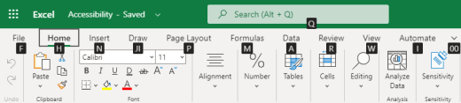
This article describes the keyboard shortcuts in Excel for the web.
Notes:
-
If you use Narrator with the Windows 10 Fall Creators Update, you have to turn off scan mode in order to edit documents, spreadsheets, or presentations with Microsoft 365 for the web. For more information, refer to Turn off virtual or browse mode in screen readers in Windows 10 Fall Creators Update.
-
To quickly find a shortcut, you can use the Search. Press Ctrl+F and then type your search words.
-
When you use Excel for the web, we recommend that you use Microsoft Edge as your web browser. Because Excel for the web runs in your web browser, the keyboard shortcuts are different from those in the desktop program. For example, you’ll use Ctrl+F6 instead of F6 for jumping in and out of the commands. Also, common shortcuts like F1 (Help) and Ctrl+O (Open) apply to the web browser — not Excel for the web.
In this article
-
Quick tips for using keyboard shortcuts with Excel for the web
-
Frequently used shortcuts
-
Access keys: Shortcuts for using the ribbon
-
Keyboard shortcuts for editing cells
-
Keyboard shortcuts for entering data
-
Keyboard shortcuts for editing data within a cell
-
Keyboard shortcuts for formatting cells
-
Keyboard shortcuts for moving and scrolling within worksheets
-
Keyboard shortcuts for working with objects
-
Keyboard shortcuts for working with cells, rows, columns, and objects
-
Keyboard shortcuts for moving within a selected range
-
Keyboard shortcuts for calculating data
-
Accessibility Shortcuts Menu (Alt+Shift+A)
-
Control keyboard shortcuts in Excel for the web by overriding browser keyboard shortcuts
Quick tips for using keyboard shortcuts with Excel for the web
-
To find any command quickly, press Alt+Windows logo key, Q to jump to the Search or Tell Me text field. In Search or Tell Me, type a word or the name of a command you want (available only in Editing mode). Search or Tell Me searches for related options and provides a list. Use the Up and Down arrow keys to select a command, and then press Enter.
Depending on the version of Microsoft 365 you are using, the Search text field at the top of the app window might be called Tell Me instead. Both offer a largely similar experience, but some options and search results can vary.
-
To jump to a particular cell in a workbook, use the Go To option: press Ctrl+G, type the cell reference (such as B14), and then press Enter.
-
If you use a screen reader, go to Accessibility Shortcuts Menu (Alt+Shift+A).
Frequently used shortcuts
These are the most frequently used shortcuts for Excel for the web.
Tip: To quickly create a new worksheet in Excel for the web, open your browser, type Excel.new in the address bar, and then press Enter.
|
To do this |
Press |
|---|---|
|
Go to a specific cell. |
Ctrl+G |
|
Move down. |
Page down or Down arrow key |
|
Move up. |
Page up or Up arrow key |
|
Print a workbook. |
Ctrl+P |
|
Copy selection. |
Ctrl+C |
|
Paste selection. |
Ctrl+V |
|
Cut selection. |
Ctrl+X |
|
Undo action. |
Ctrl+Z |
|
Open workbook. |
Ctrl+O |
|
Close workbook. |
Ctrl+W |
|
Open the Save As dialog box. |
Alt+F2 |
|
Use Find. |
Ctrl+F or Shift+F3 |
|
Apply bold formatting. |
Ctrl+B |
|
Open the context menu. |
|
|
Jump to Search or Tell me. |
Alt+Q |
|
Repeat Find downward. |
Shift+F4 |
|
Repeat Find upward. |
Ctrl+Shift+F4 |
|
Insert a chart. |
Alt+F1 |
|
Display the access keys (ribbon commands) on the classic ribbon when using Narrator. |
Alt+Period (.) |
Top of Page
Access keys: Shortcuts for using the ribbon
Excel for the web offers access keys, keyboard shortcuts to navigate the ribbon. If you’ve used access keys to save time on Excel for desktop computers, you’ll find access keys very similar in Excel for the web.
In Excel for the web, access keys all start with Alt+Windows logo key, then add a letter for the ribbon tab. For example, to go to the Review tab, press Alt+Windows logo key, R.
Note: To learn how to override the browser’s Alt-based ribbon shortcuts, go to Control keyboard shortcuts in Excel for the web by overriding browser keyboard shortcuts.
If you’re using Excel for the web on a Mac computer, press Control+Option to start.
-
To get to the ribbon, press Alt+Windows logo key, or press Ctrl+F6 until you reach the Home tab.
-
To move between tabs on the ribbon, press the Tab key.
-
To hide the ribbon so you have more room to work, press Ctrl+F1. To display the ribbon again, press Ctrl+F1.
Go to the access keys for the ribbon
To go directly to a tab on the ribbon, press one of the following access keys:
|
To do this |
Press |
|---|---|
|
Go to the Search or Tell Me field on the ribbon and type a search term. |
Alt+Windows logo key, Q |
|
Open the File menu. |
Alt+Windows logo key, F |
|
Open the Home tab and format text and numbers or use other tools such as Sort & Filter. |
Alt+Windows logo key, H |
|
Open the Insert tab and insert a function, table, chart, hyperlink, or threaded comment. |
Alt+Windows logo key, N |
|
Open the Data tab and refresh connections or use data tools. |
Alt+Windows logo key, A |
|
Open the Review tab and use the Accessibility Checker or work with threaded comments and notes. |
Alt+Windows logo key, R |
|
Open the View tab to choose a view, freeze rows or columns in your worksheet, or show gridlines and headers. |
Alt+Windows logo key, W |
Top of Page
Work in the ribbon tabs and menus
The shortcuts in this table can save time when you work with the ribbon tabs and ribbon menus.
|
To do this |
Press |
|---|---|
|
Select the active tab of the ribbon and activate the access keys. |
Alt+Windows logo key. To move to a different tab, use an access key or the Tab key. |
|
Move the focus to commands on the ribbon. |
Enter, then the Tab key or Shift+Tab |
|
Activate a selected button. |
Spacebar or Enter |
|
Open the list for a selected command. |
Spacebar or Enter |
|
Open the menu for a selected button. |
Alt+Down arrow key |
|
When a menu or submenu is open, move to the next command. |
Esc |
Top of Page
Keyboard shortcuts for editing cells
Tip: If a spreadsheet opens in the Viewing mode, editing commands won’t work. To switch to Editing mode, press Alt+Windows logo key, Z, M, E.
|
To do this |
Press |
|---|---|
|
Insert a row above the current row. |
Alt+Windows logo key, H, I, R |
|
Insert a column to the left of the current column. |
Alt+Windows logo key, H, I, C |
|
Cut selection. |
Ctrl+X |
|
Copy selection. |
Ctrl+C |
|
Paste selection. |
Ctrl+V |
|
Undo an action. |
Ctrl+Z |
|
Redo an action. |
Ctrl+Y |
|
Start a new line in the same cell. |
Alt+Enter |
|
Insert a hyperlink. |
Ctrl+K |
|
Insert a table. |
Ctrl+L |
|
Insert a function. |
Shift+F3 |
|
Increase font size. |
Ctrl+Shift+Right angle bracket (>) |
|
Decrease font size. |
Ctrl+Shift+Left angle bracket (<) |
|
Apply a filter. |
Alt+Windows logo key, A, T |
|
Re-apply a filter. |
Ctrl+Alt+L |
|
Toggle AutoFilter on and off. |
Ctrl+Shift+L |
Top of Page
Keyboard shortcuts for entering data
|
To do this |
Press |
|---|---|
|
Complete cell entry and select the cell below. |
Enter |
|
Complete cell entry and select the cell above. |
Shift+Enter |
|
Complete cell entry and select the next cell in the row. |
Tab key |
|
Complete cell entry and select the previous cell in the row. |
Shift+Tab |
|
Cancel cell entry. |
Esc |
Top of Page
Keyboard shortcuts for editing data within a cell
|
To do this |
Press |
|---|---|
|
Edit the selected cell. |
F2 |
|
Cycle through all the various combinations of absolute and relative references when a cell reference or range is selected in a formula. |
F4 |
|
Clear the selected cell. |
Delete |
|
Clear the selected cell and start editing. |
Backspace |
|
Go to beginning of cell line. |
Home |
|
Go to end of cell line. |
End |
|
Select right by one character. |
Shift+Right arrow key |
|
Select to the beginning of cell data. |
Shift+Home |
|
Select to the end of cell data. |
Shift+End |
|
Select left by one character. |
Shift+Left arrow key |
|
Extend selection to the last nonblank cell in the same column or row as the active cell, or if the next cell is blank, to the next nonblank cell. |
Ctrl+Shift+Right arrow key or Ctrl+Shift+Left arrow key |
|
Insert the current date. |
Ctrl+Semicolon (;) |
|
Insert the current time. |
Ctrl+Shift+Semicolon (;) |
|
Copy a formula from the cell above. |
Ctrl+Apostrophe (‘) |
|
Copy the value from the cell above. |
Ctrl+Shift+Apostrophe (‘) |
|
Insert a formula argument. |
Ctrl+Shift+A |
Top of Page
Keyboard shortcuts for formatting cells
|
To do this |
Press |
|---|---|
|
Apply bold formatting. |
Ctrl+B |
|
Apply italic formatting. |
Ctrl+I |
|
Apply underline formatting. |
Ctrl+U |
|
Paste formatting. |
Shift+Ctrl+V |
|
Apply the outline border to the selected cells. |
Ctrl+Shift+Ampersand (&) |
|
Apply the number format. |
Ctrl+Shift+1 |
|
Apply the time format. |
Ctrl+Shift+2 |
|
Apply the date format. |
Ctrl+Shift+3 |
|
Apply the currency format. |
Ctrl+Shift+4 |
|
Apply the percentage format. |
Ctrl+Shift+5 |
|
Apply the scientific format. |
Ctrl+Shift+6 |
|
Apply outside border. |
Ctrl+Shift+7 |
|
Open the Number Format dialog box. |
Ctrl+1 |
Top of Page
Keyboard shortcuts for moving and scrolling within worksheets
|
To do this |
Press |
|---|---|
|
Move up one cell. |
Up arrow key or Shift+Enter |
|
Move down one cell. |
Down arrow key or Enter |
|
Move right one cell. |
Right arrow key or Tab key |
|
Go to the beginning of the row. |
Home |
|
Go to cell A1. |
Ctrl+Home |
|
Go to the last cell of the used range. |
Ctrl+End |
|
Move down one screen (28 rows). |
Page down |
|
Move up one screen (28 rows). |
Page up |
|
Move to the edge of the current data region. |
Ctrl+Right arrow key or Ctrl+Left arrow key |
|
Move between ribbon and workbook content. |
Ctrl+F6 |
|
Move to a different ribbon tab. |
Tab key Press Enter to go to the ribbon for the tab. |
|
Insert a new sheet. |
Shift+F11 |
|
Switch to the next sheet. |
Alt+Ctrl+Page down |
|
Switch to the next sheet (when in Microsoft Teams or a browser other than Chrome). |
Ctrl+Page down |
|
Switch to the previous sheet. |
Alt+Ctrl+Page up |
|
Switch to previous sheet (when in Microsoft Teams or a browser other than Chrome). |
Ctrl+Page up |
Top of Page
Keyboard shortcuts for working with objects
|
To do this |
Press |
|---|---|
|
Open menu or drill down. |
Alt+Down arrow key |
|
Close menu or drill up. |
Alt+Up arrow key |
|
Follow hyperlink. |
Ctrl+Enter |
|
Open a note for editing. |
Shift+F2 |
|
Open and reply to a threaded comment. |
Ctrl+Shift+F2 |
|
Rotate an object left. |
Alt+Left arrow key |
|
Rotate an object right. |
Alt+Right arrow key |
Top of Page
Keyboard shortcuts for working with cells, rows, columns, and objects
|
To do this |
Press |
|---|---|
|
Select a range of cells. |
Shift+Arrow keys |
|
Select an entire column. |
Ctrl+Spacebar |
|
Select an entire row. |
Shift+Spacebar |
|
Extend selection to the last nonblank cell in the same column or row as the active cell, or if the next cell is blank, to the next nonblank cell. |
Ctrl+Shift+Right arrow key or Ctrl+Shift+Left arrow key |
|
Add a non-adjacent cell or range to a selection. |
Shift+F8 |
|
Insert cells, rows, or columns. |
Ctrl+Plus sign (+) |
|
Delete cells, rows, or columns. |
Ctrl+Minus sign (-) |
|
Hide rows. |
Ctrl+9 |
|
Unhide rows. |
Ctrl+Shift+9 |
|
Hide columns |
Ctrl+0 |
|
Unhide columns |
Ctrl+Shift+0 |
Top of Page
Keyboard shortcuts for moving within a selected range
|
To do this |
Press |
|---|---|
|
Move from top to bottom (or forward through the selection). |
Enter |
|
Move from bottom to top (or back through the selection). |
Shift+Enter |
|
Move forward through a row (or down through a single-column selection). |
Tab key |
|
Move back through a row (or up through a single-column selection). |
Shift+Tab |
|
Move to an active cell. |
Shift+Backspace |
|
Move to an active cell and keep the selection. |
Ctrl+Backspace |
|
Rotate the active cell through the corners of the selection. |
Ctrl+Period (.) |
|
Move to the next selected range. |
Ctrl+Alt+Right arrow key |
|
Move to the previous selected range. |
Ctrl+Alt+Left arrow key |
|
Extend selection to the last used cell in the sheet. |
Ctrl+Shift+End |
|
Extend selection to the first cell in the sheet. |
Ctrl+Shift+Home |
Top of Page
Keyboard shortcuts for calculating data
|
To do this |
Press |
|---|---|
|
Calculate workbook (refresh). |
F9 |
|
Perform full calculation. |
Ctrl+Shift+Alt+F9 |
|
Refresh external data. |
Alt+F5 |
|
Refresh all external data. |
Ctrl+Alt+F5 |
|
Apply Auto Sum. |
Alt+Equal sign ( = ) |
|
Apply Flash Fill. |
Ctrl+E |
Top of Page
Accessibility Shortcuts Menu (Alt+Shift+A)
Access the common features quickly by using the following shortcuts:
|
To do this |
Press |
|---|---|
|
Cycle between landmark regions. |
Ctrl+F6 or Ctrl+Shift+F6 |
|
Move within a landmark region. |
Tab key or Shift+Tab |
|
Go to the Search or Tell Me field to run any command. |
Alt+Q |
|
Display or hide Key Tips or access the ribbon. |
Alt+Windows logo key |
|
Edit the selected cell. |
F2 |
|
Go to a specific cell. |
Ctrl+G |
|
Move to another worksheet in the workbook. |
Ctrl+Alt+Page up or Ctrl+Alt+Page down |
|
Open the context menu. |
Shift+F10 or Windows Menu key |
|
Read row header. |
Ctrl+Alt+Shift+T |
|
Read row until an active cell. |
Ctrl+Alt+Shift+Home |
|
Read row from an active cell. |
Ctrl+Alt+Shift+End |
|
Read column header. |
Ctrl+Alt+Shift+H |
|
Read column until an active cell. |
Ctrl+Alt+Shift+Page up |
|
Read column from an active cell. |
Ctrl+Alt+Shift+Page down |
|
Open a list of moving options within a dialog box. |
Ctrl+Alt+Spacebar |
Top of Page
Control keyboard shortcuts in Excel for the web by overriding browser keyboard shortcuts
Excel for the web works in a browser. Browsers have keyboard shortcuts, some of which conflict with shortcuts that work in Excel on the desktop. You can control these shortcuts, so they work the same in both versions of Excel by changing the Keyboard Shortcuts settings. Overriding browser shortcuts also enables you to open the Excel for the web Help by pressing F1.
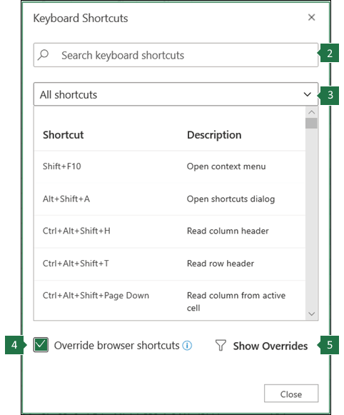
|
|
Top of Page
See also
Excel help & learning
Use a screen reader to explore and navigate Excel
Basic tasks using a screen reader with Excel
Screen reader support for Excel
Technical support for customers with disabilities
Microsoft wants to provide the best possible experience for all our customers. If you have a disability or questions related to accessibility, please contact the Microsoft Disability Answer Desk for technical assistance. The Disability Answer Desk support team is trained in using many popular assistive technologies and can offer assistance in English, Spanish, French, and American Sign Language. Please go to the Microsoft Disability Answer Desk site to find out the contact details for your region.
If you are a government, commercial, or enterprise user, please contact the enterprise Disability Answer Desk.
The videos on this channel will help you learn how to use a wide range of computer software applications ms @. particularly ms excel.data filtering and shorting in exceldata filter and shortingshorting data and filtering
short and filter datahow to shorting data and filteringexcel,ms excel
MS Excel Filter,sort u0026 filter,Excel Sort and filter,Data Sorting and Filtering in Excel,এক্সেল শর্ট ও ফিল্টার টিউটোরিয়াল,microsoft excel,
I have self-taught myself many technology topics but also have studied them at the @ level. I hold a Diploma in Marketing, a Bachelor of Education, Bachelor of Management and a Masters in Educational Technology.
Here in this video, i have explained that data filtering and shorting in excel and extract the unmatched data in a new sheet. so watch this video completely to learn data filtering and shorting in excel
:Copyright Disclaimer:
Video is for educational purpose only. Copyright Disclaimer Under Section 107 of the Copyright Act 1976, allowance is made for «fair use» for purposes such as criticism, comment, news reporting, teaching, scholarship, and research. Fair use is a use permitted by copyright statute that might otherwise be infringing. Non-profit, educational or personal use tips the balance in favor of fair use.
Contact me ;
H/P : 01734224355
Gmail : siddequr1980@gmail.com
Music in this video
Learn more
Song
Piano Trap Beethoven
Artist
josh pan
Album
Piano Trap Beethoven
Licensed to YouTube by
YouTube Audio Library
- Категория
- Инструкции
This probably never dragged too much attention because it was always there but all of a sudden you’re finding that taken-for-granted Short Date because you’ve been handed down Long Dates that contain too much information on the whole. With your worksheet bustling and your columns many in number, a Short Date format can be a needed input.
In this tutorial, you’ll find the difference between Short and Long Date formats, how to change the default Short Date format, and 3 easy ways to apply a Short Date format with Number Format on the Ribbon, Format Cells, and the TEXT function.
And first, what is the Short Date format?
 1")
What is Short Date Format in Excel
Enter the date 1-31-25 on the worksheet. The cell will snap to a date format and the entered date will snap to 1/31/2025. This Excel folk is a Short Date format and will include the shorter sides of the day, month, and year combination.
The above-mentioned format is the default, depends on the Regional format set in your computer’s Time and Language settings, English (United States) in our case. Therefore, the default format can be changed using the same settings.
With English (United States), the date components can be slightly different in other Short Date formats. The day in the Short Date format will be displayed in a single digit (1 to 31) or double digits (01 to 31). The month can be single or double digits or a 3-letter abbreviation of the month name. The year can be in double digits or in full. Any combination of these makes up a Short Date.
Short Date formats steers clear of the full month name, day name, and time which can be part of a Long Date. Other Short Date formats, with English (United States) as your computer’s Regional format setting, are listed below. All the dates are Short Date formats of the date 1st of February 2025:
Computer’s Regional format: English (United States)
| Short Date | Format | Comments |
|---|---|---|
| 1/31/2025 | m/d/yyyy | Default format |
| 2/1/25 | m/d/yy | Other formats |
| 02/01/25 | mm/dd/yy | |
| 02/01/2025 | mm/dd/yyyy | |
| 25/02/01 | yy/mm/dd | |
| 2025-02-01 | yyyy-mm-dd | |
| 01-Feb-25 | dd-mmm-yy |
Do you want know how to apply any of them?
Let’s get formatting!
How to Apply Short Date Format
If you’re at the point of data entry, all you have to do is enter the date in one of the acceptable formats and you will get a Short Date in return.
The format that the date is returned in depends on the system settings of the Regional format; English (United States) in our case. See what type of date you need to enter and the type of Short Date Excel will return:
| Date entered | Date returned |
|---|---|
| 1/31/25 | 1/31/2025 |
| 1-31-25 | 1/31/2025 |
| 2025-1-31 | 1/31/2025 |
| 31 jan 25 | 31-Jan-25 |
The returned Short Date formats are:
m/d/yyyy (the default Short Date format)
dd-mmm-yy
Depending on how the date is entered, one of two formats will be returned. When the month is entered numerically, the default Short Date format is returned i.e. m/d/yyyy. Since the default format has the month mentioned first, enter the dates month-first for them to be accepted by Excel.
When the month is entered alphabetically, the date is returned in this d/mmm/yy format with the month name abbreviated.
That’s how to deal with Short Dates when you’re creating your dataset. There’s equally the possibility that you’re dealing with ready data that has dates a mile long. There are a few quick ways you can tackle changing Long Dates to Short Dates or even if you want to change the Short Date from one format to another.
Let’s dive into the methods of applying the Short Date format to dates in Excel.
Using Number Format in Ribbon
This method applies the default Short Date format to the selected dates. Since dates are entered in the default Short Date format, the Ribbon option only concerns dates that are in a different format; whether Long or Custom.
Let’s see to this with an example we have set up with the order and delivery dates regarding the product deliveries scheduled for a slot of 6 days. For the dispatch department, the Long Date format makes more sense with the day and time mentioned. But for other departments, where reports may be drafted with many columns, we’ll try to condense the date as much as possible and that calls for the Short Date format.
To bring your dates back to the default Short Date format, use the Number Format Bar in the Ribbon with these steps:
- Select the dates that you want in the default Short Date
- Click on the Number Format Bar‘s arrow to view the Number Format menu in the Home tab’s Number
 2")
- Select the Short Date option from the menu.
 3")
And that click will switch the format of the selected dates to the default Short Date format:
 4")
Notes:
Select any date from the Short Dates and note in the Formula Bar that the actual value of the cell doesn’t change with a change in format, only the display.
The Number Format Bar will display Date as the format when the selected cell is formatted to the default Short or Long Date format.
For the formatting to work, the cell must carry a date value (which can be deduced also from the alignment to the right). If the date is copied or entered as text, Number Formats will make no changes to them.
Using Format Cells Option
You’re likely to resort to this option when you want a Short Date format but not Excel’s default one. Format Cells gives you various options for Short Date formats and also room for custom formats. This way, you can modify the placement of the date components and even add your choice of separators.
Let’s cut some dates short. Use the Format Cells option to apply a Short Date format in Excel with the following steps:
- Select the cells containing the dates you want to reformat.
- From the Ribbon, select the dialog launcher of the Home tab’s Number group to access the Format Cells dialog box.
- Using the Number group’s launcher opens the Format Cells dialog box in the Number tab directly.
 5")
- In the dialog box, go through the format types in the Date category to choose a Short Date format of preference.
 6")
If you’ve found what you want, use the OK button to apply it but would this even be a neat tutorial without giving you more ideas?
At this point, you can use the Locale (location) to get a location-specific format which may include the locale’s native language in the date.
We talked about custom formats earlier and now would be the best time to collate one by heading to the Custom category. Before that, picking a format from the Date category first will allow you to edit that format in the Custom category.
- Go to the Custom category and it will carry the formatting code of the format selected in the Date
 7")
- Use the code as a base to edit it into a custom code for a Custom Short Date
- We will change the separator from a hyphen to a period and change the day component from «d» to «dd» so that the day will be displayed in double digits instead of a single digit. 1 will be displayed as 01; look at the Sample box before and after editing the code to see a preview of this change.
 8")
- Hit the OK command in the dialog box.
The dates will now have a custom Short Date format, also confirmed by the Number Format Bar:
 9")
That’s the good thing about formatting; the dates will be usable in calculations and date formulas. When it won’t be a good thing is the case of wanting to use the date as text. This is Excel so a lot of these notions should be possible, right? This innocent notion can come true thanks to the TEXT function so read up ahead!
Using TEXT Function
The TEXT function can return the date as a Short Date in text format. The date needs to be the only value present in the cell so that the function knows what to pick on. The TEXT function converts the cell value to text in the supplied format. We will feed the TEXT function with our choice of Short Date format so it can return the Long Dates as Short Dates in text form.
Dates won’t always need to be used in calculations and you may need the date to be a part of a text to go on a receipt, footnote, or email message for example. There was also something we said about rearranging the components of the date so let’s see what the TEXT function can do for us. Enter the formula below to use the TEXT function to apply a Short Date format:
=TEXT(C3,"m/d/yyyy")
Columns C and D in our case example have the original Long Dates. Taking the first date in C3, we’ve applied the format «m/d/yyyy» with the year component placed first, enclosed in double quotes. All the rest of the Long Dates in the dataset also follow:
 10")
The Number Format Bar also shows that the resulting value is not in a date format anymore. Now you can pick the text from here and place it as text wherever needed.
Formulas for other short date formats
It’s not just the default Short Date format that the TEXT function will be able to work with. You can go with any other Short Date format of preference or the format that conforms to the default Short Date format as per your computer’s Regional format settings. Enter the relevant Short Date format in the formula such as:
=TEXT(B3,"dd-mmm-yy")
See how this would apply to a Long Date:
 11")
If you’re going totally unconventional, the TEXT function can accept that too like this formula below:
=TEXT(B3,"yyyy| mmm dd")
This Short Date format has the date components regrouped and separated with the vertical bar. Here’s how it worked out in Excel:
 12")
How to Change Default Short Date Format
By now, we’re well familiar that the default Short Date format is m/d/yyyy. This format being the default is resultant of the Regional format set as English (United States). The format may change by changing this setting but you can also change the default Short Date format leaving the Regional format untouched. Either way, these are the steps to go about if you want to change the default Short Date format:
- Visit the Start Menu of your computer and select the Settings
- Select Time & Language on the Settings
 13")
- Now select the Region tab from the pane on the left.
This is the part you’re interested in when it comes to some default settings of your computer such as the Short and Long Date and time formats, the region, the first day of the week, etc.
If you change the region in the Regional format setting, this may also automatically change the default Short Date format e.g. the default format for a Short Date with English (United Kingdom) as the Regional format is dd/mm/yyyy.
But keeping the Regional format constant, you can still change the default Short Date format and for that, proceed with these steps:
- At the bottom of the Region settings click on the last option reading Change data formats.
 14")
- Click on the arrow of the Short Date bar and select a different format for the default Short Date.
 15")
Regional format data will instantly be updated.
 16")
Now when a date is entered in Excel, the new default format for the Short Date will be applied and you can confirm this change from the Number Format Bar which shows the updated default Short Date format:
 17")
Short Date Format vs Long Date Format
The Short Date format does not include the full month name, only the 3-letter abbreviation at most. By default, the representation of the month component is numerical. The Long Date format displays the complete month name and may show the day name and time.
The Short Date format is applied by default to dates whereas the Long Date format is applied by the user. A Short Date entered that takes on the default format will be a date value that can be used in calculations and date functions.
The Short Date format has the date components divided by a separator (forward slash or hyphen mostly) after the first and second components in the date. The Long Date format includes commas as the separator by default.
Use the Short Date format to quickly enter the date and also where you would prefer to have compact dates and narrow columns. Use the Long Date format to feature the day, full month, or time for quick analysis.
To sum it up shortly, the Short Date format is applied by default to a date entered in Excel. It can be customized to be displayed differently and can be converted to text and is space efficient. While you’re chipping at your Excel Long Dates to shorten them, we’ll come up with more Excel chiseling, hacking away at another problem!
The problem is that you have too many columns and rows in your Excel sheet and you are wasting a lot of valuable space. You want to shorten it. So, we are here to help.
Below we will cover what you need, some good tips on how to proceed, and finally step-by-step instructions on how to shorten your spreadsheet.
- Ways To Shorten the Spreadsheet
- Resize Excel File
- How To Set the End of an Excel Spreadsheet
- Reduce Excel File Size Without Opening
- Compress Excel Files Offline
- Excel File Size Limit
- Reduce the file size of your Excel workbook
- Why is My Excel File So Large
- FAQ
- How To Reduce Excel File Size by Deleting Blank Rows?
- How Do I Remove Thousands of Rows in Excel?
- How Do I Adjust the Length in Excel?
- Conclusion
Ways To Shorten the Spreadsheet
- Delete unnecessary cells e.g. empty columns, rows
- Hide unnecessary columns and rows
- Stretch the hidden columns and rows back so everything is compact again
Here are some tips for your reference:
Tip1: Use AutoFilter to quickly find the empty columns and rows
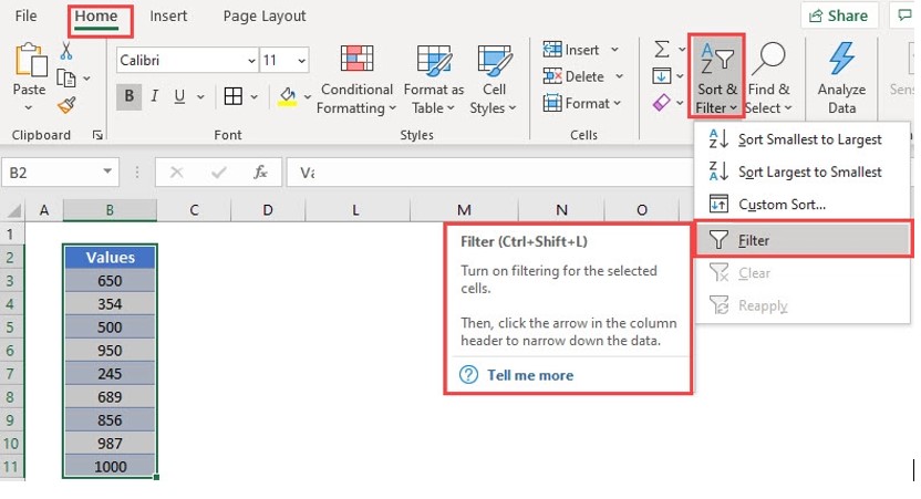
Tip2: Use the Conditional Formatting feature to help you easily find and delete unnecessary cells
You may want to delete some unnecessary cells quickly before you proceed with hiding some other columns and rows. Please use AutoFilter to quickly find blank cells.
- Start the search from the cell you want
- In the lower-left corner, choose the ‘Filter’ button
- Then click on Cell > Filter (the AutoFilter button)
- Choose the filter criteria. For example, if you want to find empty columns, use “Column” as the filter criteria and remember to apply it to all of your blank columns.
Tip3: Use conditional formatting to hide unnecessary columns and rows with one click.
If you want to hide unnecessary cells quickly, the conditional formatting feature will be helpful. Please start with normal Excel and then use the rest of the article to alter your spreadsheet and hide unnecessary columns and rows.
- First, check if conditional formatting is available in your version of Excel. For example, if you have an older version of Excel (or a trial version), then you may not have it at all.
- After that, select the cells to format.
- In the ribbon, click the ‘Conditional Formatting’ button
- On the ‘Conditional Formatting dialog box, choose a rule from the first drop-down list and choose a color from the second list. Additionally, you can adjust other parameters.
- Click ‘OK’.
- Check out your spreadsheet and you will find that the unnecessary cells are now hidden.
Resize Excel File
- You can see this file size is 20.5MB. We are gonna convert this file.
- Open the sheet and go to file
- Click the save as
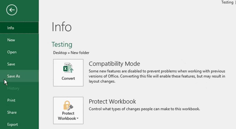
- Select Browse
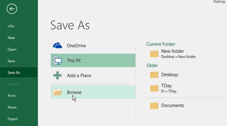
- Select your output location
- Change the file name if necessary
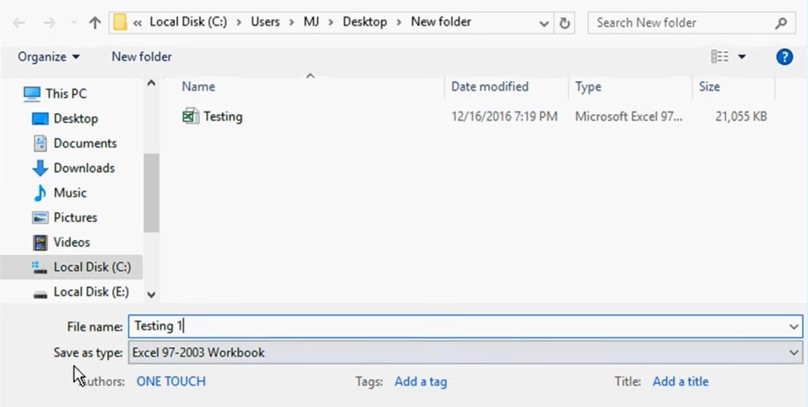
- After that select ‘excel binary workbook’ in the ‘save as type
- Save the file
- This 20.5MB file turned into a 2.38MB file
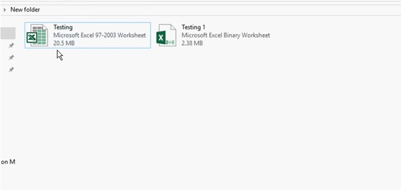
- Open the file and check
This is the most straightforward way to shorten your excel sheet.
How To Set the End of an Excel Spreadsheet
Excel allows you to set the end of your workbook so that when you save it, only the data on the sheet is saved. You can set a different “End” for each sheet in your workbook. This way, if a sheet contains confidential information, will be hidden.
Setting Excel’s “End” is easy and only takes a few seconds to do. Let’s see how to do it for a single sheet as well as for all sheets in your workbook.
- Open your workbook.
- Select the sheet that you want to set the end for (e.g. sheet “A”) and then right-click on it.
- In the drop-down menu choose “End Of This Worksheet”
- Now you should see the end of your sheet set at this location
- Save the workbook with a new file name.
- Close it and open it again to see if the end of it has changed to where you clicked in Step 4 above as shown below:
- The End of Sheet “#A” has been changed at this location now!
- Now click on “File -> Save As…,” and save the file with a new name.
- Close it and open it again to see that the end of it has changed to where you clicked in Step 4 above.
Reduce Excel File Size Without Opening
Excel has a feature to compress/encrypt workbooks. When you enable password protection on your workbook, it also compresses the file.
The original data (and formatting) are maintained. Only the size is reduced. You can still open the file, it’s just smaller. You can surely read or update the data and format it in Excel.
Enable Encryption/Compression
- Click the File tab, then click Save As.
- Under Encryption (possible only if you have a version that supports this feature), select either 128-bit or 256-bit encryption.
- Select the current location or specify a new location, and then click Save.
- The file is saved in your specified location with a .xlsx extension. Now you can safely move it to different places, send it via email or store it on the computer or network drives.
Compress Excel Files Offline
If you want to compress/compress your Excel files offline, you can use the built-in ZIP function to achieve the same result.
NOTE: If you compress your Excel files offline, they can be read on any computer that has Office installed.
The ZIP function can be found in the menu on the right-hand side of the Excel ribbon.
- Click the Zip button after selecting the file.
- Your desktop will be saved with compressed files.
Excel File Size Limit
Excel provides a built-in feature that allows you to increase/decrease the file size limit of Excel for all files in Excel.
- Click File -> Options-> Save tab.
- Under General, limit the file size to < 4GB.
- To check it, save a workbook with a large number of rows and columns, close Excel, and re-open it. If the file size exceeds the limit, it should be deleted.
You can also increase/decrease the limit on a particular workbook by using this technique:
- Go to File: Go -> New, select Save As, and click the More Options button.
- Change the Maximum size field and click OK.
- Select the new workbook and close Excel.
- Open your new workbook which is now smaller than your may have wanted it to be, save it again, and re-open Excel.
- You can confirm that the file size is now smaller by using Save As.
Reduce the file size of your Excel workbook
Why is My Excel File So Large
There are many reasons why your Excel file size is exorbitantly large, and the reason is generally not related to the data in the file. Your Excel file size could be full of junk data, and waste space or it could also be because you have some very valuable (but rarely used) features turned on that are contributing a large amount of unnecessary space.
The good news is, you can easily reduce your Excel file size without any loss of data, and with very little effort on your part.
Autoformatting can be a major culprit for large Excel files. The best way to control the mess in your spreadsheet is to disable Autoformats as soon as possible. This is because Autoformats are always changing (even if you don’t change them), and are also using up tons of unnecessary space.
FAQ
How To Reduce Excel File Size by Deleting Blank Rows?
Delete extra rows and columns to reduce your Excel file size.
You can use the Delete option to delete extra rows and columns, but this may affect the format of your spreadsheet.
- Select a blank cell or cell range (not containing any values or formatting)
- Press Ctrl + Del, duplicate rows or columns, and then delete the summarized cells.
- Check out your spreadsheet to ensure that you have not deleted any cells you wanted.
- Now you have the desired blank cells or cell range.
- Change the formatting and enter the data in the cells or cell range you want.
How Do I Remove Thousands of Rows in Excel?
If you have a large number of rows in your data file, you can try the following technique to reduce the number of rows.
- Select a cell in the bottom half of your data range
- Use Ctrl + Home and Ctrl +End to select all cells above and below this cell.
- Delete the selected range (all cells from where you are currently working downwards)
- Save and exit Excel.
How Do I Adjust the Length in Excel?
- Go to File: Go -> New, select Save As, and click the More Options button.
- Navigate to Tools -> Publisher and then select Custom Size.
- For Width and Height, enter an integer value. Do not include a unit or the value will change when you move the focus back to Excel.
- Save your new workbook and re-open it.
- You will see that the width of your workbook has changed to the specified width and the height for the new length you have entered.
- Now you can start filling the cells with data, or in this case, there is a very small number of rows that occupy a large portion of your Excel file (literally thousands), it would also be a good idea to delete them because these are just wasting space.
- Find a blank cell or a cell range that is not part of your required data, and then delete it.
- Update any formatting as required.
This technique can also be used to reduce the amount of data you are working with if you are trying to reduce the size of your Excel file by removing rows and columns.
Conclusion
Now that you know how to shorten your spreadsheet, you should be able to do so.
If you want to reduce the size of your Excel file, you should use the functions and features provided by Microsoft Office’s AutoFit feature. The AutoFit feature will allow you to customize the rows and columns in your spreadsheet so that it does not change when you open or save a file.
This reduces the amount of wasted space in your data because it will allow Excel to store only what is necessary. That’s how to do it easily.
Bottom line: Learn some of my favorite keyboard shortcuts when working with rows and columns in Excel.
Skill level: Easy
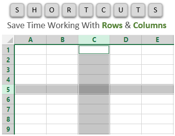
Whether you are creating a simple list of names or building a complex financial model, you probably make a lot of changes to the rows and columns in the spreadsheet. Tasks like adding/deleting rows, adjusting column widths, and creating outline groups are very common when working with the grid.
This post contains some of my favorite shortcuts that will save you time every day.
I’ve also listed the equivalent shortcuts for the Mac version of Excel where available.
#1 – Select Entire Row or Column
Shift+Space is the keyboard shortcut to select an entire row.
Ctrl+Space is the keyboard shortcut to select an entire column.
Mac Shortcuts: Same as above
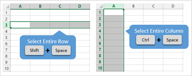
The keyboard shortcuts by themselves don’t do much. However, they are the starting point for performing a lot of other actions where you first need to select the entire row or column. This includes tasks like deleting rows, grouping columns, etc.
These shortcuts also work for selecting the entire row or column inside an Excel Table.
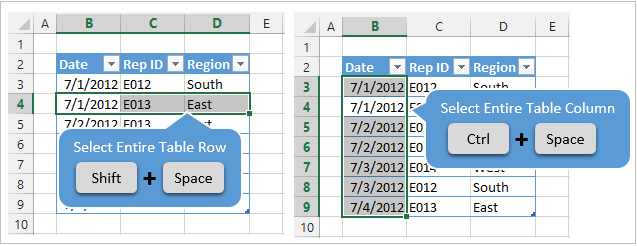
When you press the Shift+Space shortcut the first time it will select the entire row within the Table. Press Shift+Space a second time and it will select the entire row in the worksheet.
The same works for columns. Ctrl+Space will select the column of data in the Table. Pressing the keyboard shortcut a second time will include the column header of the Table in the selection. Pressing Ctrl+Space a third time will select the entire column in the worksheet.
You can select multiple rows or columns by holding Shift and pressing the Arrow Keys multiple times.
![]()
#2 – Insert or Delete Rows or Columns
There are a few ways to quickly delete rows and columns in Excel.
If you have the rows or columns selected, then the following keyboard shortcuts will quickly add or delete all selected rows or columns.
Ctrl++ (plus character) is the keyboard shortcut to insert rows or columns. If you are using a laptop keyboard you can press Ctrl+Shift+= (equal sign).
Mac Shortcut: Cmd++ or Cmd+Shift+
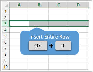
Ctrl+- (minus character) is the keyboard shortcut to delete rows or columns.
Mac Shortcut: Cmd+-
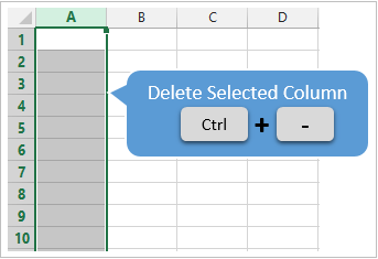
So for the above shortcuts to work you will first need to select the entire row or column, which can be done with the Shift+Space or Ctrl+Space shortcuts explained in #1.
If you do not have the entire row or column selected then you will be presented with the Insert or Delete Menus after pressing Ctrl++ or Ctrl+-.
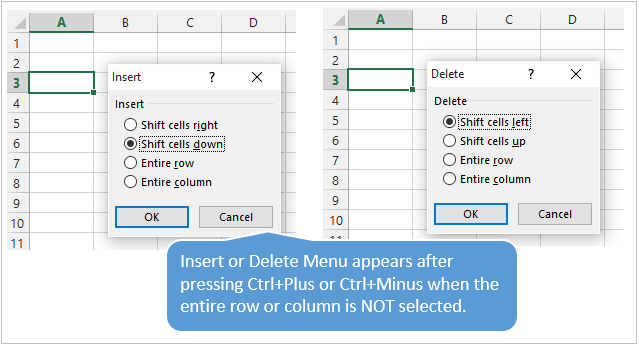
You can then press the up or down arrow keys to make your selection from the menu and hit Enter. For me it is easier to first select the entire row or column, then press Ctrl++ or Ctrl+-.
So, the entire keyboard shortcut to delete a column would be Ctrl+Space, Ctrl+-. You could also use the keyboard shortcut Alt+H+D+C to delete columns and Alt+H+D+R to delete rows. There are lots of ways to do a simple task… 🙂
#3 – AutoFit Column Width
There are also a lot of different ways to AutoFit column widths. AutoFit means that the width of the column will be adjusted to fit the contents of the cell.
You can use the mouse and double-click when you hover the cursor between columns when you see the resize column cursor.
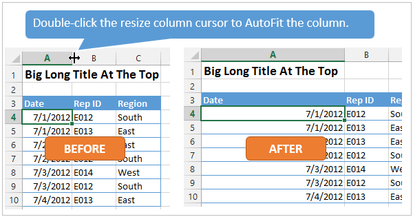
The problem with this is that you might just want to resize the column for the date in cell A4, instead of the big long title in cell A1. To accomplish this you can use the AutoFit Column Width button. It is located on the Home tab of the Ribbon in the Format menu.
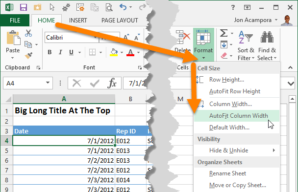
The AutoFit Column Width button bases the width of the column on the cells you have selected. In the image above I have cell A4 selected. So the column width will be adjusted to fit the contents of A4, as shown in the results below.
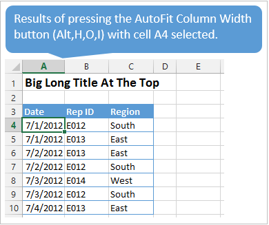
Alt,H,O,I is the keyboard shortcut for the AutoFit Column Width button. This is one I use a lot to get my reports looking shiny. 🙂
Alt,H,O,A is the keyboard shortcut to AutoFit Row Height. It doesn’t work exactly the same as column width, and will only adjust the row height to the tallest cell in the entire row.
Mac Shortcuts: None that I know of. The Mac version does not use the Alt key sequence which I believe is a limitation of the Mac OS.
#3.5 – Manually Adjust Row or Column Width
The column width or row height windows can be opened with keyboard shortcuts as well.
Alt,O,R,E is the keyboard shortcut to open the Row Height window.
Alt,O,C,W is the keyboard shortcut to open the Column Width window.
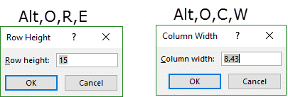
The row height or column width will be applied to the rows or columns of all the cells that are currently selected.
These are old shortcuts from Excel 2003, but they still work in the modern versions of Excel.
Mac Shortcuts: None that I know of. The Mac version does not use the Alt key sequence which I believe is a limitation of the Mac OS.
#4 – Hide or Unhide Rows or Columns
There are several dedicated keyboard shortcuts to hide and unhide rows and columns.
- Ctrl+9 to Hide Rows
- Ctrl+0 (zero) to Hide Columns
- Ctrl+Shift+( to Unhide Rows
- Ctrl+Shift+) to Unhide Columns – If this doesn’t work for you try Alt,O,C,U (old Excel 2003 shortcut that still works). You can also modify a Windows setting to prevent the conflict with this shortcut. See the comment from Pablo Baez on Oct 5, 2015 below for further instructions. Thanks Pablo! 🙂
Mac Shortcuts: Same as above
The buttons are also located on the Format menu on the Home tab of the Ribbon. You can hover over any of the items in the menu and the keyboard shortcut will display in the screentip (see screenshot below).
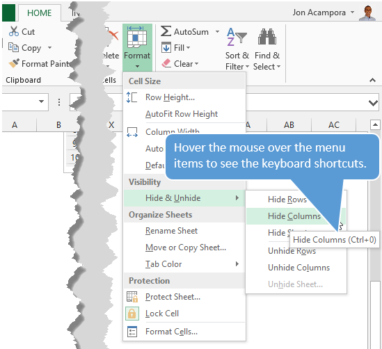
The trick with getting these shortcuts to work is to have the proper cells selected first.
To hide rows or columns you just need to select cells in the rows or columns you want to hide, then press the Ctrl+9 or Ctrl+Shift+( shortcut.
To unhide rows or columns you first need to select the cells that surround the rows or columns you want to unhide. In the screenshot below I want to unhide rows 3 & 4. I first select cell B2:B5, cells that surround or cover the hidden rows, then press Ctrl+Shift+( to unhide the rows.
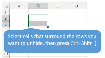
The same technique works to unhide columns.
#5 – Group or Ungroup Rows or Columns
Row and Column groupings are a great way to quickly hide and unhide columns and rows.
Shift+Alt+Right Arrow is the shortcut to group rows or columns.
Mac Shortcut: Cmd+Shift+K
Shift+Alt+Left Arrow is the shortcut to ungroup.
Mac Shortcut: Cmd+Shift+J
Again, the trick here is to select the entire rows or columns you want to group/ungroup first. Otherwise you will be presented with the Group or Ungroup menu.
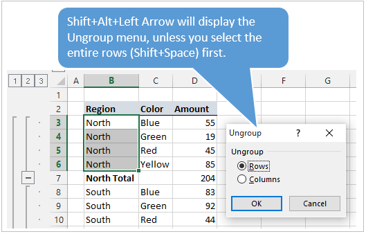
Alt,A,U,C is the keyboard shortcut to remove all the row and columns groups on the sheet. This is the same as pressing the Clear Outline button on the Ungroup menu of the Data tab on the Ribbon.
*Bonus funny: At some point when using the group/ungroup shortcuts, you will accidentally press Ctrl+Alt+Right Arrow. This is a Windows shortcut that orientates the entire screen to the right. I call it “neck ache view”. To get it back to normal press Ctrl+Alt+Up Arrow.
If your co-worker or boss accidentally leaves their computer unlocked and you want to play a joke on them, press Ctrl+Alt+Down Arrow. This will turn their screen upside down. Don’t forget to record a video of their WTF reaction… 🙂
What Are Your Favorites?
There are a ton of keyboard shortcuts for working with rows and columns. The above are some of my favorites that I use everyday. What are some of your favorites? Please leave a comment below. Thanks! 🙂
![]()
Download Article
![]()
Download Article
This wikiHow teaches you how to shorten the appearance of data in Microsoft Excel. To do this, your full, unshortened data will need to be entered into Excel first.
-
1
Open Microsoft Excel. If you have an existing document with your data already entered, you can double-click it to open it; otherwise, you’ll need to open a new workbook and enter your data now.
-
2
Select the cell where you want the truncated text to appear. This method is useful for text that you already have in your spreadsheet.
- Note that this cell must be different than the cell in which your target text appears.
Advertisement
-
3
Type the LEFT or RIGHT formula into your selected cell. The LEFT and RIGHT formula are built on the same premise, though the LEFT formula displays characters from the left side of your cell’s text and the RIGHT formula displays characters from the right. The formula is «=DIRECTION(Cell Name, Number of characters to display)» without the quotation marks. For example:[1]
- =LEFT(A3, 6) displays the first six characters in cell A3. If the text in A3 says «Cats are better», the truncated text will read «Cats a» in your selected cell.
- =RIGHT(B2, 5) displays the last 5 characters in cell B2. If the text in B2 says «I love wikiHow», the truncated text will read «kiHow» in your selected cell.
- Keep in mind that spaces count as characters.
-
4
Press Enter when the formula is complete. Your selected cell will automatically fill with the truncated text.


Advertisement
-
1
Select the cell where you want the truncated text to appear. This cell must be different than the cell in which your target text appears.
- If you haven’t already added your data to Excel, you’ll need to do so first.
-
2
Type the MID formula into your selected cell. MID chops characters off of the beginning and end of your selected cell’s text. To set up the MID formula, you type «=MID(Cell Name, Starting Character Number, Number of characters to display)» without the quotation marks. For example:
- =MID(A1, 3, 3) displays three characters from cell A1, the first of which is the third character from the left in the text. If A1’s text says «racecar», the truncated text will read «cec» in your selected cell.
- Similarly, =MID(B3, 4, displays eight characters from cell B3, starting with the fourth character from the left. If B3’s text says «bananas aren’t people», the truncated text will read «anas are» in your selected cell.
-
3
Press Enter when the formula is complete. This will add the truncated text to your selected cell.


 displays eight characters from cell B3, starting with the fourth character from the left. If B3’s text says «bananas aren’t people», the truncated text will read «anas are» in your selected cell.
Advertisement
-
1
Select the cell you wish to split up. This should be a cell that has more characters than space.
-
2
Click Data. It’s in the toolbar at the top of your Excel page.
-
3
Select Text to Columns. You’ll find this option in the «Data Tools» section of the Data tab.
- This function divides the cell’s contents of one Excel cell into separate columns.
-
4
Select Fixed Width. After clicking on Text to Columns window will pop up, called «Convert Text to Columns Wizard Step 1 of 3.» The window will have two selections: «Delimited» and «Fixed Width.» Delimited means that characters, such as tabs or commas will divide each field. You will usually select delimited when you’re importing data from another application, such as a database. The fixed width option means that the fields are lined up in columns that have spaces between the individual field.
-
5
Click Next. This window shows three options. If you want to create a break line, click on the position where you want the text to break. If you want to delete the break line, double click on the line. To adjust the line, click and drag it around the data.
-
6
Click Next. This window has several options, «General», «Text,» «Date» and «Do not import column (skip).» Unless you want to force your cell’s formatting to do something different than its natural state, you can skip this page.
-
7
Click Finish. Your text should now be divided between two or more cells.


Advertisement
Add New Question
-
Question
How do I remove all the text after a period?

It depends on whether it is the first period possible, or a later one. I will address it being the first period as the alternatives are a little involved. Use the LEFT() function. The thing you need to work hard for is where is the period? For that, you can use the FIND() function which will locate its position. Since you want precisely that many characters fro the left of the text, nothing more is needed. = LEFT( A1, FIND( «.», A1 ) ). You can use FIND() this way for many things.
-
Question
How can I change all instances of a word to a letter in Excel?
Use the SUBSTITUTE() function, with the word you wish to change into a letter being the text to go away («old_text») and the letter you desire in their places being the text to put in place («new_text»).
Ask a Question
200 characters left
Include your email address to get a message when this question is answered.
Submit
Advertisement
Thanks for submitting a tip for review!
About This Article
Article SummaryX
1. Select the cell where you want the truncated text to appear.
2. Type the LEFT or RIGHT formula in the cell.
3. Press Enter.
Did this summary help you?
Thanks to all authors for creating a page that has been read 481,241 times.
Is this article up to date?
When you type something like 2/2 in a cell, Excel for the web thinks you’re typing a date and shows it as 2-Feb. But you can change the date to be shorter or longer. To see a short date like 2/2/2013, select the cell, and then click Home > Number Format > Short Date.
Contents
- 1 How do I create a short date in Excel?
- 2 What is short date and long date?
- 3 What is short format date?
- 4 What is long date excel?
- 5 How do I convert a short date to a long date in Excel?
- 6 What is a long date format?
- 7 What is Z in date format?
- 8 How do I change a date format from DD MM to yyyy in Excel?
- 9 Which date format is this?
- 10 How do I change a cell to a short date format?
- 11 What date is yyyy-mm-dd?
- 12 How do I use currency 0 in Excel?
- 13 How do you shorten dates?
- 14 What is the long date today?
- 15 What are date functions in Excel?
- 16 Why is Excel showing instead of date?
- 17 Why is my date not formatting in Excel?
- 18 Where is quick analysis tool in Excel?
- 19 What is DDD in date?
- 20 How do you write a long date?
How do I create a short date in Excel?
Short Date Format in Excel
- Excel provides different ways of displaying dates, be it short date, long date or a customized date.
- Click Home tab, then click the drop-down menu in Number Format Tools.
- Select Short Date from the drop-down list.
- The date is instantly displayed in short date format m/d/yyyy.
What is short date and long date?
Long Date(“D”) Format Specifier. The “D” standard format specifier represents a custom date and time format string defined by the DateTimeFormatInfo. ShortDatePattern property. The custom format string for the Short Date Format Specifier is “dddd , dd MMMM yyyy”.
Short format: dd/MM/yy (Example: 13/06/03) Medium format: dd/MM/yyyy (Example: 13/06/2003) Long format: d’ de ‘MMMM’ de ‘yyyy (Example: 13 de junio de 2003)
What is long date excel?
The long date option adds the day of the week and writes out the month. So 1/1/19 will display as Tuesday, January 1, 2019. The date will display in the format you choose, no matter how you enter it. If you type “1/1/19” into a cell with the long date format, Excel will change it to the expanded date.
How do I convert a short date to a long date in Excel?
To quickly change date format in Excel to the default formatting, do the following:
- Select the dates you want to format.
- On the Home tab, in the Number group, click the little arrow next to the Number Format box, and select the desired format – short date, long date or time.
What is a long date format?
Long Date. Displays only date values, as specified by the Long Date format in your Windows regional settings. Monday, August 27, 2018. Medium Date. Displays the date as dd/mmm/yy, but uses the date separator specified in your Windows regional settings.
What is Z in date format?
Z is the zone designator for the zero UTC offset. “09:30 UTC” is therefore represented as “09:30Z” or “T0930Z”. “14:45:15 UTC” would be “14:45:15Z” or “T144515Z”. The Z suffix in the ISO 8601 time representation is sometimes referred to as “Zulu time” because the same letter is used to designate the Zulu time zone.
How do I change a date format from DD MM to yyyy in Excel?
To change the date display in Excel follow these steps:
- Go to Format Cells > Custom.
- Enter dd/mm/yyyy in the available space.
Which date format is this?
Date Format Types
| Format | Date order | Description |
|---|---|---|
| 1 | MM/DD/YY | Month-Day-Year with leading zeros (02/17/2009) |
| 2 | DD/MM/YY | Day-Month-Year with leading zeros (17/02/2009) |
| 3 | YY/MM/DD | Year-Month-Day with leading zeros (2009/02/17) |
| 4 | Month D, Yr | Month name-Day-Year with no leading zeros (February 17, 2009) |
How do I change a cell to a short date format?
Follow these steps:
- Select the cells you want to format.
- Press CTRL+1.
- In the Format Cells box, click the Number tab.
- In the Category list, click Date.
- Under Type, pick a date format.
- If you want to use a date format according to how another language displays dates, choose the language in Locale (location).
What date is yyyy-mm-dd?
Date/Time Formats
| Format | Description |
|---|---|
| MM/DD/YY | Two-digit month, separator, two-digit day, separator, last two digits of year (example: 12/15/99) |
| YYYY/MM/DD | Four-digit year, separator, two-digit month, separator, two-digit day (example: 1999/12/15) |
How do I use currency 0 in Excel?
Format numbers as currency in Excel for the web
- Select the cells that you want to format and then, in the Number group on the Home tab, click the down arrow in the Number Format box.
- Choose either Currency or Accounting.
How do you shorten dates?
16. How dates are written and abbreviated
- In most countries of the world, dates are written in order DAY/MONTH/YEAR, e.g., 4 July 1999, abbreviated 4/7/1999.
- In eastern Asia, however, dates are written in order YEAR/MONTH/DAY: 1999 July 4, abbreviated 1999/7/4.
What is the long date today?
Today’s Date
| Today’s Date in Other Date Formats | |
|---|---|
| Unix Epoch: | 1639391773 |
| RFC 2822: | Mon, 13 Dec 2021 02:36:13 -0800 |
| DD-MM-YYYY: | 13-12-2021 |
| MM-DD-YYYY: | 12-13-2021 |
What are date functions in Excel?
The DATE function is an Excel function that combines three separate values (year, month, and day) to form a date. When used along with other Excel functions, it can be used to perform a wide range of tasks related to dates, including returning specified dates.
Why is Excel showing instead of date?
Microsoft Excel might show ##### in cells when a column isn’t wide enough to show all of the cell contents. Formulas that return dates and times as negative values can also show as #####.If dates are too long, click Home > arrow next to Number Format, and pick Short Date.
Why is my date not formatting in Excel?
If you want to sort the dates, or change their format, you’ll have to convert them to numbers – that’s how Excel stores valid dates. Sometimes, you can fix the dates by copying a blank cell, then selecting the date cells, and using Paste Special > Add to change them to real dates.
Where is quick analysis tool in Excel?
Whenever you select a cell range, the Quick Analysis button will appear in the lower-right corner of the selection. When you click it, you’ll be able to choose from a variety of charts, sparklines, conditional formatting options, and more.
What is DDD in date?
The “ddd” custom format specifier represents the abbreviated name of the day of the week. The localized abbreviated name of the day of the week is retrieved from the DateTimeFormatInfo. AbbreviatedDayNames property of the current or specified culture.
How do you write a long date?
Sometimes, a date is written in long form, like this: Sunday, June 28, 2015 (note that there are commas after the day of the week and the day of the month, but there is no comma after the month). Sometimes, a date is written in numerical form, like this: 6/28/15 or 6/28/2015 (month/date/year).