
Excel for Microsoft 365 Excel 2021 Excel 2019 Excel 2016 Excel 2013 Excel 2010 Excel 2007 More…Less
If your worksheet has a lot of columns, you can use the Scale to Fit options to reduce the size of the worksheet to better fit the printed page.
Follow these steps:
-
Click the Page Layout tab on the ribbon.
-
In the Scale to Fit group, in the Width box, select 1 page, and in the Height box, select Automatic. Columns will now appear on one page, but the rows may extend to more than one page.

To print your worksheet on a single page, choose 1 page in the Height box. Keep in mind, however, that the printout may be difficult to read because Excel shrinks the data to fit. To see how much scaling is used, look at the number in the Scale box. If it’s a low number, you may need to make other adjustments before you print. For example, you may need to change the page orientation from portrait to landscape or target a larger paper size. For more information, see the section below to understand a few things about scaling a worksheet to fit a printed page.
-
To print your worksheet, press CTRL+P to open the Print dialog box, and then click OK.

For the best experience as you scale a worksheet, it is important to remember the following:
-
If your worksheet has many columns, you may need to switch the page orientation from portrait to landscape. To do this, go to Page Layout > Page Setup > Orientation, and click Landscape.
-
Consider using a larger paper size to accommodate many columns. To switch the default paper size, go to Page Layout > Page Setup > Size, and then choose the size you want.
-
Use the Print Area command (Page Setup group) to exclude any columns or rows that you don’t need to print. For example, if you want to print columns A through F, but not columns G through Z, set the print area to include only columns A through F.
-
You can shrink or enlarge a worksheet for a better fit on printed pages. To do that, in Page Setup, click the window launcher button. Then, click Scaling > Adjust to, and then enter the percentage of the normal size that you want to use.
Note: To reduce a worksheet to better fit the printed pages, enter a percentage that is smaller than 100%. To enlarge a worksheet to fit the printed pages, enter a percentage greater than 100%.
-
Page Layout view isn’t compatible with the Freeze Panes command. If you don’t want to unfreeze the rows or columns in your worksheet, you can skip Page Layout view and instead use the Fit to options on the Page tab in the Page Setup dialog box. To do that, go to Page Layout tab, and in the Page Setup group, click the Dialog Box Launcher
at the bottom-right side. Optionally, press ALT+P, S, P on the keyboard. -
To print a worksheet on a specific number of pages, in Page Setup, click the small window launcher button. Then, under Scaling, in both of the Fit to boxes, enter the number of pages (wide and tall) on which you want to print the worksheet data.
Notes:
-
Excel ignores manual page breaks when you use the Fit to option.
-
Excel does not stretch the data to fill the pages.
-
-
To remove a scaling option, go to File > Print > Settings > No Scaling.
 at the bottom-right side. Optionally, press ALT+P, S, P on the keyboard.
When you print an Excel worksheet, you may find that the print font size is not what you expect.
Follow these steps to scale the worksheet for print by increasing or decreasing its font size.
-
In the worksheet, click File > Print.
-
Under Settings, click Custom Scaling > Custom Scaling Options.
-
Click Page and in the Adjust to box, choose a percentage by which you want to increase or decrease the font size.
-
Review your changes in Print Preview and—if you want a different font size—repeat the steps.
Note: Before you click Print, check the paper size setting in the printer properties, and also make sure the printer actually has paper in that size. If the paper size setting is different from the paper size in your printer, Excel adjusts the printout to fit the paper size in the printer and the printed worksheet might not match your Print Preview
In Print Preview, if the worksheet appears to be reduced to a single page, check if a scaling option like Fit Sheet on One Page has been applied. Refer to the section above to learn how to make adjustments.
Need more help?
You can always ask an expert in the Excel Tech Community or get support in the Answers community.
See Also
Quick start: Print a worksheet
Need more help?
Want more options?
Explore subscription benefits, browse training courses, learn how to secure your device, and more.
Communities help you ask and answer questions, give feedback, and hear from experts with rich knowledge.
Scale a worksheet
- Click the Page Layout tab on the ribbon.
- In the Scale to Fit group, in the Width box, select 1 page, and in the Height box, select Automatic.
- To print your worksheet, press CTRL+P to open the Print dialog box, and then click OK.
Contents
- 1 How do I scale an Excel spreadsheet on one page?
- 2 What is Excel scale to fit?
- 3 How do you change the magnification of a worksheet in Excel?
- 4 How do I change the scale in Excel?
- 5 How do I fix scaling issues in Excel?
- 6 How do I put a footer in Excel?
- 7 Where is quick analysis tool in Excel?
- 8 How do I create a scale in Excel?
- 9 How do I scale a column in Excel?
- 10 How do you scale 120 in Excel?
- 11 What is zoom control in Excel?
- 12 What is formula bar and worksheet in MS Excel?
- 13 How do I change the horizontal scale in Excel?
- 14 How do I change the chart range in Excel?
- 15 How do I change the y axis values in Excel?
- 16 How do you adjust screen scaling?
- 17 How do I fix screen scaling?
- 18 What is scaling in Windows 10?
- 19 How do I add a footer to all sheets in Excel?
- 20 How do you fill handle in Excel?
How do I scale an Excel spreadsheet on one page?
Shrink a worksheet to fit on one page
- Click Page Layout.
- Select the Page tab in the Page Setup dialog box.
- Select Fit to under Scaling.
- To fit your document to print on one page, choose 1 page(s) wide by 1 tall in the Fit to boxes.
- Press OK at the bottom of the Page Setup dialog box.
What is Excel scale to fit?
When you think of scaling to fit, especially when using MS Excel, the first thing that comes to mind is to shrink the content so it fits on one piece of paper. However, scaling means to shrink or enlarge.
How do you change the magnification of a worksheet in Excel?
When you want to quickly change the magnification of a worksheet, use the Zoom slider. You’ll find the Zoom slider in the bottom right corner of the Excel window. To use the Zoom slider, drag the slider to the right or to the left. To zoom in, drag the slider to the right.
How do I change the scale in Excel?
You can change the scale used by Excel by following these steps:
- Right-click on the axis whose scale you want to change. Excel displays a Context menu for the axis.
- Choose Format Axis from the Context menu.
- Make sure the Scale tab is selected.
- Adjust the scale settings, as desired.
- Click on OK.
How do I fix scaling issues in Excel?
Select Display > Change the size of text, apps, and other items, and then adjust the slider for each monitor. Right-click the application, select Properties, select the Compatibility tab, and then select the Disable display scaling on high DPI settings check box.
On the Insert tab, in the Text group, click Header & Footer. Excel displays the worksheet in Page Layout view. To add or edit a header or footer, click the left, center, or right header or footer text box at the top or the bottom of the worksheet page (under Header, or above Footer). Type the new header or footer text.
Where is quick analysis tool in Excel?
Whenever you select a cell range, the Quick Analysis button will appear in the lower-right corner of the selection. When you click it, you’ll be able to choose from a variety of charts, sparklines, conditional formatting options, and more.
How do I create a scale in Excel?
How to Draw to Scale in Excel
- Open Excel and click the “File” menu.
- Click the “Insert” menu and then click the “Picture” button.
- Click the “Insert” tab and then click the “Shapes” button to display a gallery of shapes you can use to trace the inserted image.
How do I scale a column in Excel?
Resize columns
- Select a column or a range of columns.
- On the Home tab, in the Cells group, select Format > Column Width.
- Type the column width and select OK.
How do you scale 120 in Excel?
In the worksheet, click File > Print. Under Settings, click Custom Scaling > Custom Scaling Options. Click Page and in the Adjust to box, choose a percentage by which you want to increase or decrease the font size.
What is zoom control in Excel?
Zoom control is a slider that lies next to view buttons at the right end of the status bar. It helps zoom in and zoom out the document. Move the slider to right or click on the plus sign to zoom in and move it to left or click on the minus sign to zoom out.
What is formula bar and worksheet in MS Excel?
The Formula Bar in Excel sits directly above the worksheet area, to the right of the Name Box. The formula bar can be used to edit the content of any cell and can be expanded to show multiple lines for the same formula (example, shortcut for toggling).
How do I change the horizontal scale in Excel?
- Click anywhere in the chart. This displays the Chart Tools, adding the Design and Format tabs.
- On the Format tab, in the Current Selection group, click the arrow in the box at the top, and then click Horizontal (Category) Axis.
How do I change the chart range in Excel?
On the ribbon, click Chart Design and then click Select Data. This selects the data range of the chart and displays the Select Data Source dialog box. To edit a legend series, in the Legend entries (series) box, click the series you want to change. Then, edit the Name and Y values boxes to make any changes.
How do I change the y axis values in Excel?
How to Change the Axis Range
- Select the axis that we want to edit by left-clicking on the axis.
- Right-click and choose Format Axis.
- Under Axis Options, we can choose minimum and maximum scale and scale units measure.
- Format axis for Minimum insert 15,000, for Maximum 55,000.
How do you adjust screen scaling?
To change a display scaling size using the recommended settings, use these steps:
- Open Settings.
- Click on System.
- Click on Display.
- Under the “Scale and layout” section, use the drop-down menu and select the scale settings that suit your needs. Options available include 100, 125, 150, and 175 percent.
How do I fix screen scaling?
Open the Start menu and select Settings. Go to System. In Display, check the Scale and Resolution options, and adjust them to make your screen look proper. Setting to an option labeled (Recommended) is often the best choice.
What is scaling in Windows 10?
The Windows 10 display scaling system adjusts the size of text, icons, and navigation elements to make a computer easier for people to see and use. You can adjust the display scaling for your Windows 10 device, as well as for any external displays.
Insert a Footer in Excel
If you want to add a footer to an Excel spreadsheet, click the “Insert” tab on the ribbon menu. Then click “Header & Footer” within the “Text” group of options. Click the header or footer on the page and type in the text you want.
How do you fill handle in Excel?
To use the fill handle:
- Select the cell(s) containing the content you want to use. The fill handle will appear as a small square in the bottom-right corner of the selected cell(s).
- Click, hold, and drag the fill handle until all of the cells you want to fill are selected.
- Release the mouse to fill the selected cells.
Asked by: Elsa Hahn
Score: 4.3/5
(60 votes)
In the worksheet, click File > Print. Under Settings, click Custom Scaling > Custom Scaling Options. Click Page and in the Adjust to box, choose a percentage by which you want to increase or decrease the font size. Review your changes in Print Preview and—if you want a different font size—repeat the steps.
What is scaling on Excel?
Scale to Fit Print Options
When you think of scaling to fit, especially when using MS Excel, the first thing that comes to mind is to shrink the content so it fits on one piece of paper. However, scaling means to shrink or enlarge.
How do I create a scale in Excel?
How to Draw to Scale in Excel
- Open Excel and click the «File» menu. …
- Click the «Insert» menu and then click the «Picture» button. …
- Click the «Insert» tab and then click the «Shapes» button to display a gallery of shapes you can use to trace the inserted image.
How do you unlock the scale in Excel?
On the Home tab, click the Format Cell Font popup launcher. You can also press Ctrl+Shift+F or Ctrl+1. In the Format Cells popup, in the Protection tab, uncheck the Locked box and then click OK. This unlocks all the cells on the worksheet when you protect the worksheet.
Why is Excel printing so small?
Step 1: Open your spreadsheet in Excel 2013. … The Print Preview at the right side of the window should adjust, and your spreadsheet should now appear larger than it previously did. If your spreadsheet is printing fine, but is either too small or too large on your screen, then you might need to adjust the zoom level.
21 related questions found
How do I fix the print scale?
How To Set Scaling (Reduce/Enlarge) Options for Print Jobs
- In the Printer Properties window, select Printing Options.
- Click on the Paper, and then select Other Size > Advanced Paper Size > Scaling Options.
- Select an option: No Scaling: This option does not change the size of the printed image. …
- Click OK.
How do I put a footer in Excel?
On the Insert tab, in the Text group, click Header & Footer. Excel displays the worksheet in Page Layout view. To add or edit a header or footer, click the left, center, or right header or footer text box at the top or the bottom of the worksheet page (under Header, or above Footer). Type the new header or footer text.
How do you scale to fit in Excel on a Mac?
Print a sheet on just one page in Excel for Mac
- On the Page Layout tab, select Page Setup.
- Under Scaling, select Fit to, and type 1 in both the page(s) wide box and page(s) tall box. Select OK. .
- On the File menu, select Print.
What does page scale mean?
Scaling is a word that means stretching or shrinking the image to fit a specified area, and it is accomplished by simply changing the value of the number used as resolution when the printer calculates the spacing of the dots on the paper.
Why is my print out so small?
If printed text is too small or the entire page prints in a smaller size than expected, change the font size or page scale settings in the application you are printing from. … Font type and text size settings must be changed in the application you are printing from.
What is Page Scaling on a printer?
Page scaling lets you shrink or enlarge pages when you print. You can: Automatically scale to fit the paper. Manually scale by percentages.
Where is print scaling on word?
This feature works the same in all modern versions of Microsoft Word: 2010, 2013, and 2016. On the Print page in Backstage view, under Settings , select the fifth drop-down that by default says Letter . Then select a scaling option.
How do I increase cell size in Excel?
Select the row or rows that you want to change. On the Home tab, in the Cells group, click Format. Under Cell Size, click Row Height. In the Row height box, type the value that you want, and then click OK.
How do I adjust the print area in Excel?
Set one or more print areas
- On the worksheet, select the cells that you want to define as the print area. Tip: To set multiple print areas, hold down the Ctrl key and click the areas you want to print. …
- On the Page Layout tab, in the Page Setup group, click Print Area, and then click Set Print Area.
How do I scale the whole page in Excel?
Shrink a worksheet to fit on one page
- Click Page Layout. …
- Select the Page tab in the Page Setup dialog box.
- Select Fit to under Scaling.
- To fit your document to print on one page, choose 1 page(s) wide by 1 tall in the Fit to boxes. …
- Press OK at the bottom of the Page Setup dialog box.
Where is quick analysis tool in Excel?
To use the Quick Analysis tool, all you have to do is select the worksheet table’s cells and then click the Quick Analysis tool that automatically appears in the lower-right corner of the last selected cell. When you do, a palette of options (from Formatting to Sparklines) appears right beneath the tool.
What is the shortcut to adjust width in Excel?
To change the column width, press Alt+O and then press C (for Column) and then W (for width). Type your values and press Enter. In Excel 2007, press Alt, which puts Excel into a shortcut key mode (see the January 2009 column, page 74, for more on the use of KeyTips) and press H for the Home tab of the Ribbon.
How do you unlock an Excel spreadsheet for editing?
Unprotect an Excel worksheet
- Go to File > Info > Protect > Unprotect Sheet, or from the Review tab > Changes > Unprotect Sheet.
- If the sheet is protected with a password, then enter the password in the Unprotect Sheet dialog box, and click OK.
How do you scale?
To scale an object to a larger size, you simply multiply each dimension by the required scale factor. For example, if you would like to apply a scale factor of 1:6 and the length of the item is 5 cm, you simply multiply 5 × 6 = 30 cm to get the new dimension.
How do you find the scale of a drawing?
The scale is shown as the length in the drawing, then a colon («:»), then the matching length on the real thing. Example: this drawing has a scale of «1:10», so anything drawn with the size of «1» would have a size of «10» in the real world, so a measurement of 150mm on the drawing would be 1500mm on the real horse.
How do I increase the font size in Excel?
Scale a worksheet to print in a different font size
- In the worksheet, click File > Print.
- Under Settings, click Custom Scaling > Custom Scaling Options.
- Click Page and in the Adjust to box, choose a percentage by which you want to increase or decrease the font size.
The term normalization in itself is a buzzword that is popular amongst people who come from different fields such as Machine Learning, Data Science, Statistics, etc. Normalization is a general term that means to scale down values inside a certain range. The origin of the word normalization being a buzzword comes from the fact that it is often misunderstood by people and is interchangeably used with another statistical term standardization. In this article, we are going to demystify both of these terms and later we will read how we can implement these techniques on a sample dataset in Excel.
Normalization (Or Min-Max scaling) data in excel
It is the process of scaling data in such a way that all data points lie in a range of 0 to 1. Thus, this technique, makes it possible to bring all data points to a common scale. The mathematical formula for normalization is given as:
 , where X is the data point, Xmax and Xmin are the maximum and minimum value in the group of records respectively. The process of normalization is generally used when the distribution of data does not follow the Gaussian distribution.
Let’s have a look at one example to see how can we perform normalization on a sample dataset. Suppose, we have a record of the height of 10 students inside a class as shown below:
| Height (in cm) |
| 152 |
| 155 |
| 168 |
| 175 |
| 153 |
| 162 |
| 173 |
| 166 |
| 158 |
| 156 |
Step 1: Calculate the minimum value in the distribution. It can be calculated using the MIN() function. The minimum value comes out to be 152 which is stored in the B14 cell.
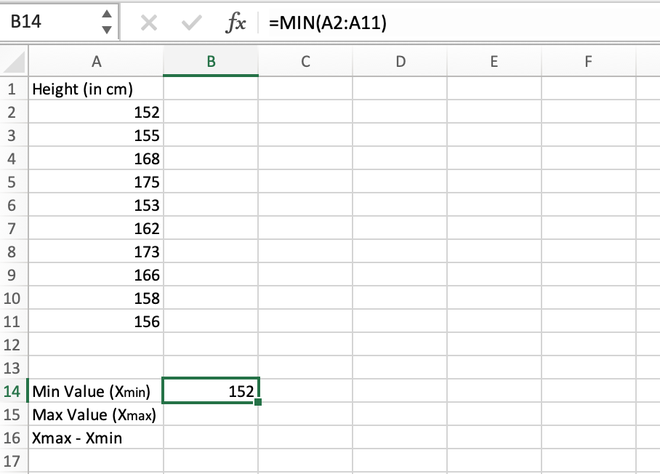
Calculating the minimum value using the MIN() function
Step 2: Calculate the maximum value in the distribution. It can be calculated using the MAX() function. The maximum value comes out to be 175 which is stored in the B15 cell.
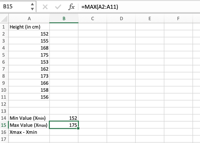
Calculating the maximum value using the MAX() function
Step 3: Find the difference between the maximum and minimum values. Their difference comes out to be 175 – 152 = 23 which is stored in the B16 cell.
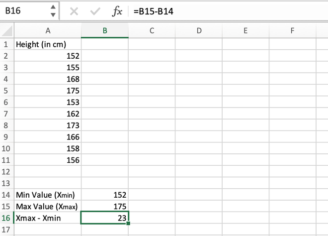
Calculating the difference (Max-Min)
Step 4: For the first data stored in the A2 cell, we will calculate the normalized value as shown in the below video.
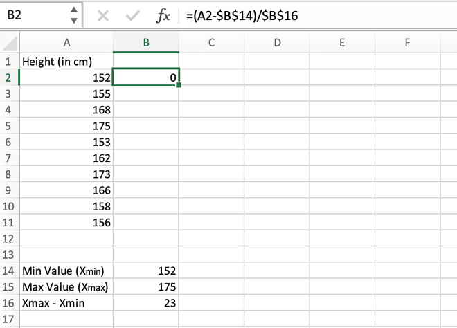
Calculating the normalized value for the first element
Step 5: We can manually calculate all values one by one for each data record or we can directly get values for all the other cells using the auto-fill feature of Excel. For this, go to the right corner of the B2 cell until a (+) symbol appears, and then drag the cursor to the bottom to auto-populate values inside all the cells.
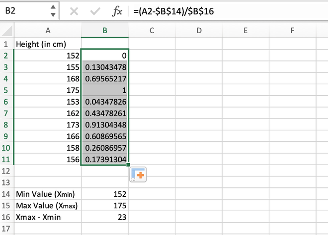
Calculating the normalized value for the entire range
Note: While calculating the first normalized value in the B2 cell, it should be made sure that the reference address for the B14 and B16 cells should be locked using Fn + F4 button otherwise an error will be thrown.
If we have a close look at the results, we can notice all the values lies in the range 0 to 1.
Standardization (Or Z-score normalization)
Standardization is a process in which we want to scale our data in such a way that the distribution of our data has its mean as 0 and standard deviation as 1. The mathematical formula for standardization is given as:
 , where where X is the data point, Xmean is the mean of the distribution and σx is the standard deviation of the distribution.
The process of standardization is generally used when we know the distribution of data follows the gaussian distribution.
Method 1: Calculating z-score normalization manually
Step 1: Calculate the mean/average of the distribution. It can be done using the AVERAGE() function. The mean value comes out to be 161.8 and is stored in the B14 cell.
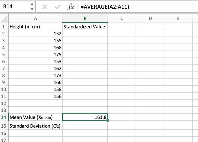
Calculating the mean value using the AVERAGE() function
Step 2: Calculate the standard deviation of the distribution which can be done using the STDEV() function. The standard deviation comes out to be 8.323994767 which is stored in the B15 cell.
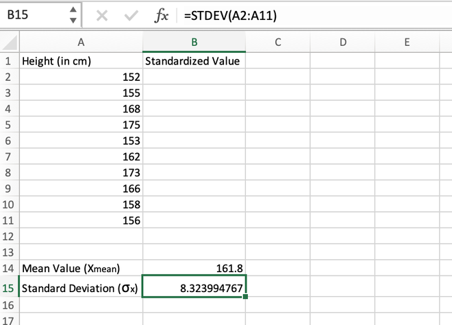
Calculating the standard deviation using the STDEV() function
Step 3: For the first data stored in the A2 cell, we will calculate the standardized value as shown in the image given below.
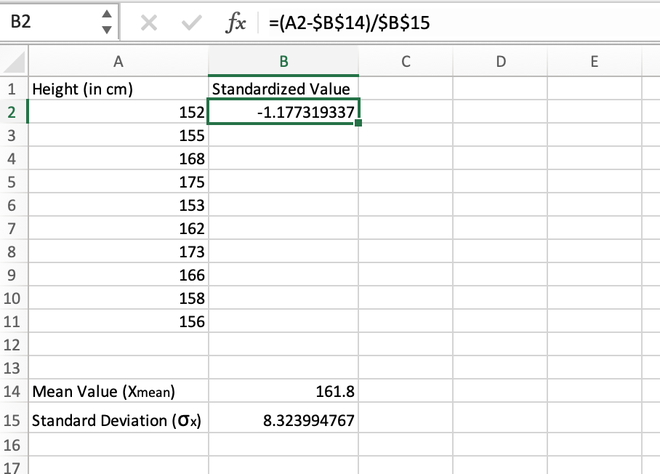
Calculating the standardized value for the first element
Step 4: After manually calculating the first value, we can simply use the auto-fill feature of Excel to populate the standardized values for all other records.
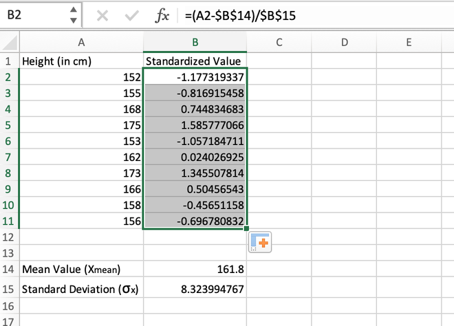
Calculating the standardized value for the entire range using auto-fill
Note: While calculating the first standardized value in the B2 cell, it should be made sure that the reference address for the B14 and B15 cells should be locked using Fn+F4 button otherwise an error will be thrown.
Method 2: Calculating Z-score normalization using the STANDARDIZE() function
We can even use the built-in STANDARDIZE() function to find the standardized value of an element. The syntax for STANDARDIZE() function is given as:
=STANDARDIZE(x,mean,std_dev)
Where x is the specific element/range of cells, mean is the average/arithmetic mean of all the elements in the record, and std_dev is the standard deviation of all the elements in the record
Step 1: Calculate the mean/average of the distribution. It can be done using the AVERAGE() function. The mean value comes out to be 161.8 and is stored in the B14 cell.
Calculating the mean value using the AVERAGE() function
Step 2: Calculate the standard deviation of the distribution which can be done using the STDEV() function. The standard deviation comes out to be 8.323994767 which is stored in the B15 cell.
Calculating the standard deviation using the STDEV() function
Step 3: For the first data stored in the A2 cell, we will calculate the standardized value as shown in the below image.
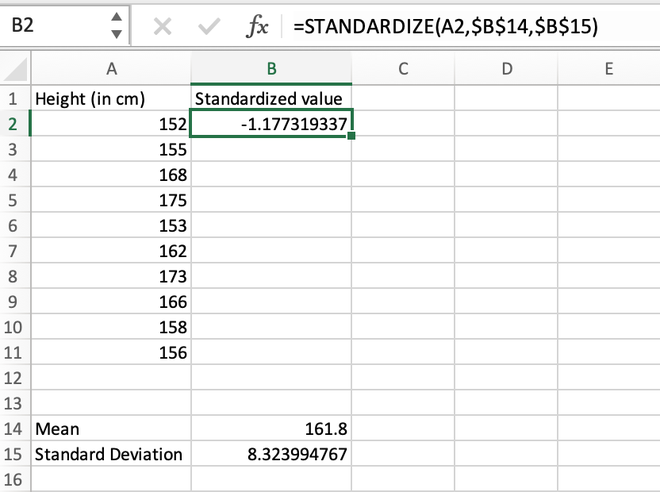
Calculating the standardized value for the first element using the STANDARDIZE() function
Step 4: After manually calculating the first value, we can simply use the auto-fill feature of Excel to populate the standardized values for all other records.
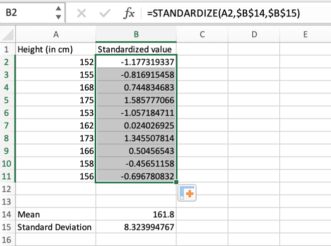
Calculating the standardized value for the entire range using auto-fill
Excel is one of the office tools we use the most of the Microsoft Office package. Without this program, there are tasks that would be very difficult; but thanks to its functions they become simple. Today you will learn to calculate or represent a scale in Excel.
What is a scale and what is it used for?
A scale, is defined as the mathematical relationship that there is between the real size of a place or object and a drawing represented on a plan, diagram or map. It is widely used in jobs related to geography, architecture, engineering or the military.
exist 3 types: natural scale, reduction and enlargement. The first has a 1 to 1 relationship (the drawing and the object are the same); the second is when the object is larger than the drawing and the third is the opposite case.
The scales are represented by 2 separate quantities by a colon (:). The first figure corresponds to the size of the plan or drawing, and the second to the real dimension. So, on a 1: 1000 scale, each centimeter of the plane represents a real thousand centimeters.
What is and why do we use a function in Excel?
You may also be interested in:
Functions in Excel they are actually formulas that come predefined, to do calculations using values in an already established order. In many cases, those values come from specific cells that the user places in the formula.
 1")
Basically they are composed of 3 parts: an equals symbol (=), the name of the function, and the values that the function needs enclosed in parentheses.
For example: = SUM (B1: C1). Here we tell the SUM function to add the values of its arguments, which in this case are cells B1 and C1; the result will be seen in the cell where this formula is applied.
Even if your job requires it, you can even make a graph in Excel by taking data from multiple sheets easily. Which is why Excel has remained a essential tool in offices.
It is important to take into account that the function name will change depending on language of your Microsoft Office; Well, if it is in English, the same SUM function will be SUM and the same will happen with the other Excel functions.
How to calculate or represent a scale in Excel?
Excel has a extensive list of functions, which are used to perform calculations and comparisons. For example, some very useful and common ones are the COUNTIF function in Excel, and also the logical AND (AND) function in Excel. But today you will see a new one for the scales.
In Excel we can easily calculate a scale using a formula that will include the GCF function. Since in this way we will obtain the minimum value resulting from the division, which represents the scale adequately.
GCF is a mathematical function that returns the greatest common divisor that there are between 2 or more numbers (maximum 29 numbers). We can insert it in 3 ways: from «Formulas> Insert function> GCD», also in «Formulas> Mathematics and trigonometrics> GCD», or press the Insert function button in the formula bar.
 2")
This feature is available in all versions of Excel. It is a native Excel function and easy to locate. The formula would be the following: = A2 / GCD (A2: B2) & «:» & B2 / GCD (A2: B2)
The arguments of the MCD function are the values of the cells A2 and B2, which have the scales of drawing and reality respectively. The ampersand symbol (&) is used to join or concatenate the results of each calculation; the colon (:) are placed as a text string, so they are enclosed in double quotes (“).
Therefore, if we have a table of several values, we will have to apply this same formula but adapted at each pair of scale values; changing only the arguments of the formula, that is, the cells that contain the values.
It is easy to calculate or represent a scale in Excel; just enough follow the instructions step by step. Now for example, you can place the scales of a map, and then import the Excel sheets into Google Docs to share your work. We hope this information is useful and that you share it with your friends.
You may also be interested in: