27
27 people found this article helpful
What Is The Ribbon In Excel?
Make the display fit the way you work
Updated on January 12, 2020
First introduced in Excel 2007, the ribbon is the strip of buttons and icons located above the work area. The ribbon replaces the menus and toolbars found in earlier versions of Excel.
Instructions in this article apply to Excel for Microsoft 365, Excel 2019, Excel 2016, Excel 2013, and Excel 2010.
Ribbon Components
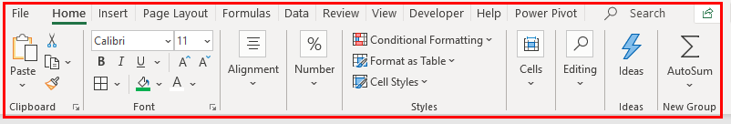
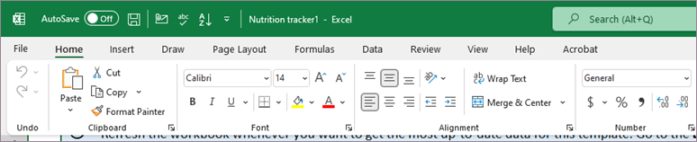
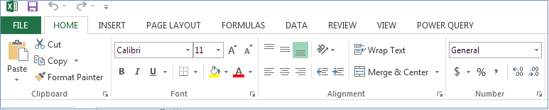
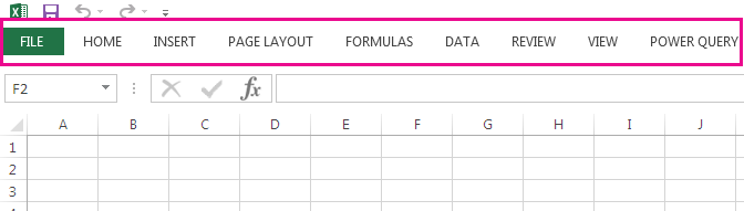
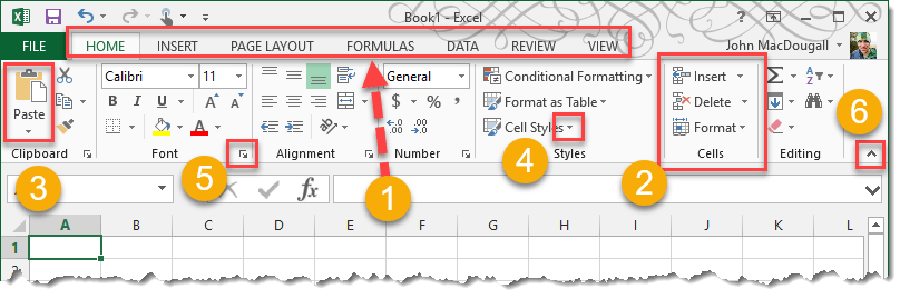
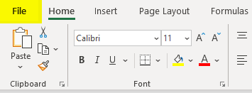
The ribbon includes tabs labeled Home, Insert, Page Layout, Formulas, Data, Review, View, and Help. When you select a tab, the area below the ribbon displays a set of groups and, within the groups, buttons representing a variety of commands.
When Excel opens the Home tab displays, along with the groups and buttons within it. Each group represents a function. The Number group includes commands that format numbers, for example, to increase or decrease the number of decimal places. The Cells group includes options to insert, delete, and format cells.
Selecting a command on the ribbon may lead to further options contained in a contextual menu or dialog box that relate to the chosen command.
Collapse and Expand the Ribbon
The ribbon can be collapsed to increase the size of the worksheet visible on the computer screen.
There are four ways to collapse the ribbon:
- Double-click a ribbon tab, such as Home, Insert, or Page Layout to display only the tabs. To expand the ribbon, double-click a tab.
- Press CTRL+F1 on the keyboard to display only the tabs. To expand the ribbon, press CTRL+F1.
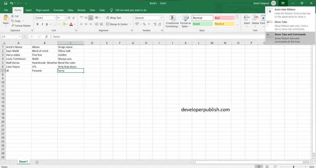
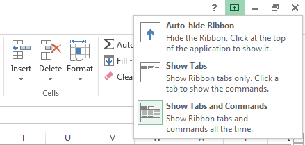
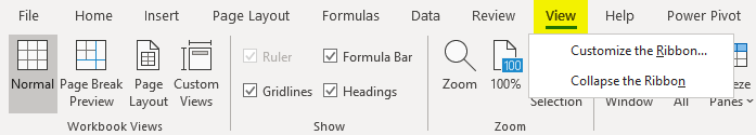
- Select Ribbon Display Options (located above the ribbon in the upper-right corner of Excel and looks like a box with an up-facing arrow) and choose Auto-hide Ribbon. Neither the tabs nor the commands will be visible. To expand the ribbon, select Ribbon Display Options, and choose Show Tabs and Commands.
- Select the up arrow located on the right side of the ribbon to collapse the ribbon and display only the tabs. To expand the ribbon, double-click a tab.
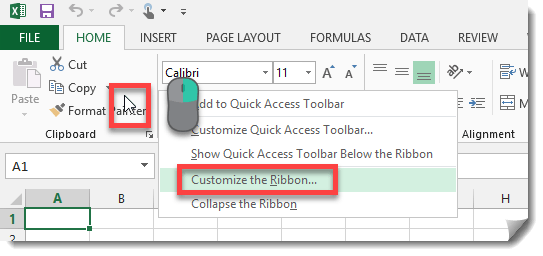
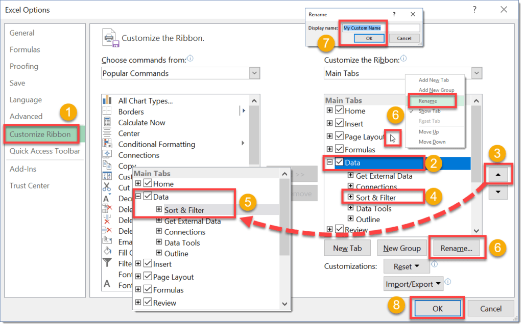
Customize the Ribbon
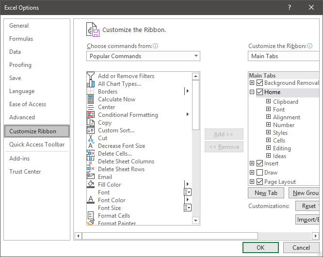
Since Excel 2010, it has been possible to customize the ribbon using the Customize Ribbon option. Use this option to:
- Rename or reorder the default tabs and groups.
- Display certain tabs.
- Add or remove commands to existing tabs.
- Add custom tabs and custom groups that contain frequently used commands.
There are also command features that cannot be changed on the ribbon, specifically the default commands which appear in gray text in the Customize Ribbon window, for example:
- Names of the default commands.
- Icons associated with the default commands.
- The order of these commands on the ribbon.
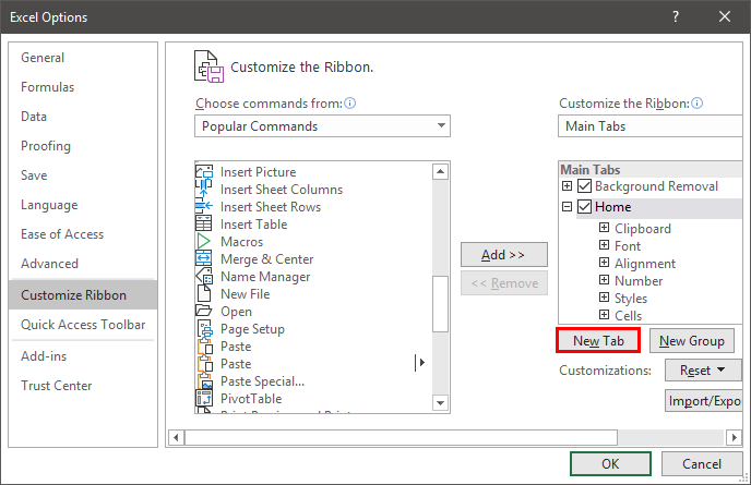
To add commands to the ribbon:
-
Select a tab, such as Home, Insert, or Page Layout.
-
Right-click a blank area of the ribbon.
-
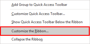
Select Customize the Ribbon.
-
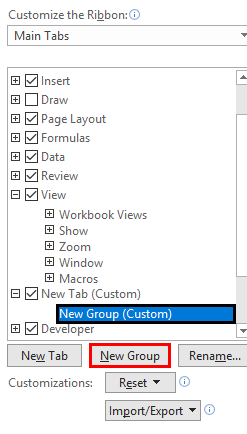
Go to the Main Tabs list and select the tab (for example the Layout tab) to which you want to add a command. Then select New Group.
When adding commands to the ribbon, you must create a custom group.
-
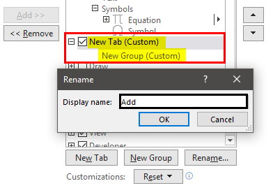
A New Group (Custom) item appears under the tab you selected. To give the group a more specific name, select Rename.
-
In the Rename window, select an icon, then go to the Display name text box and enter a descriptive name for the command. Select OK.
-
Select the group you just created.
-
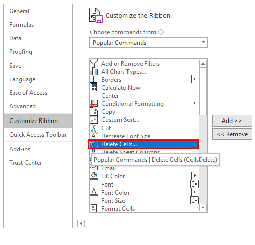
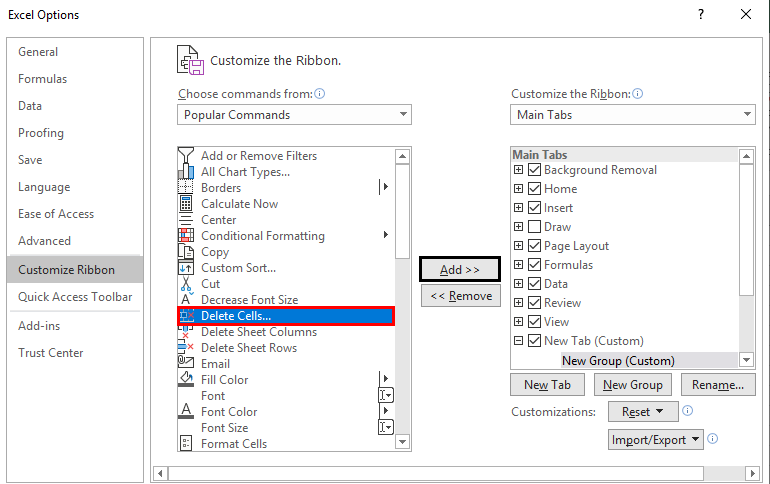
In the Choose commands from list, choose the command to add to this group, then select Add.
-
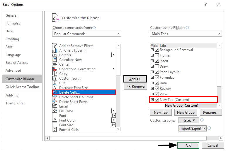
Select OK. The new group and command appear on the ribbon.
Thanks for letting us know!
Get the Latest Tech News Delivered Every Day
Subscribe
First introduced in Excel 2007, the ribbon is the strip of buttons and icons located above the work area. The ribbon replaces the menus and toolbars found in earlier versions of Excel.
Contents
- 1 What is the definition of ribbon in Excel?
- 2 How many ribbons are in Excel?
- 3 What is Ribbon command?
- 4 What is the main function of the ribbons?
- 5 What are the 3 components of ribbon?
- 6 How do I create a ribbon in Excel?
- 7 Where is ribbon in Excel?
- 8 What are the main components of Excel ribbon?
- 9 What are the parts of ribbon?
- 10 Where do you find the ribbon?
- 11 What is ribbon in computer for class 3?
- 12 What is the difference between ribbon and toolbar?
- 13 What best describes a ribbon?
- 14 What’s another name for ribbon?
- 15 What is the importance of ribbon display options?
- 16 What is a ribbon menu?
- 17 What are the 7 tabs of the ribbon?
- 18 What are the 8 tabs of the ribbon?
- 19 How do I make my own ribbon?
- 20 What is the meaning of ribbon in computer?
What is the definition of ribbon in Excel?
Microsoft Excel ribbon is the row of tabs and icons at the top of the Excel window that allows you to quickly find, understand and use commands for completing a certain task.Ribbon tab contains multiple commands logically sub-divided into groups.
How many ribbons are in Excel?
There are nine tabs on the Excel Ribbon: File, Home, Insert, Page Layout, Formulas, Data, Review, View, and Help. The Home tab is the default tab when Excel is opened. Now let’s go through each tab, from left to right, to understand each of their features.
What is Ribbon command?
What Is The Command Ribbon? The Ribbon is Excel’s command menu interface. It organizes commonly used actions together in an intuitive and visual way. These are the main parts of the Ribbon. Tabs organize related groups of commands together.
What is the main function of the ribbons?
The purpose of the ribbon is to provide quick access to commonly used tasks within each program. Therefore, the ribbon is customized for each application and contains commands specific to the program. Additionally, the top of the ribbon includes several tabs that are used to reveal different groups of commands.
What are the 3 components of ribbon?
Using the Ribbon
There are five main components to a Ribbon; QAT (Quick Access Toolbar), tabs, command buttons, groups of command buttons, and dialog launchers.
How do I create a ribbon in Excel?
To customize the Ribbon, open or create an Excel, Word, or PowerPoint document. Go to the app Preferences and select Ribbon and Toolbar. On the Ribbon tab window, select the commands you want to add or remove from your Ribbon and select the add or remove arrows.
Click the Ribbon Display Options icon on the top-right corner of your document. It is to the left of the Minimize icon. In the menu that opens, click Show Tabs and Commands to show the Ribbon with all tabs and full commands.
What are the main components of Excel ribbon?
Four main components of Excel Ribbon are Tabs, Groups, Buttons and Dialog Box launcher.
What are the parts of ribbon?
There are five main components to a Ribbon; QAT (Quick Access Toolbar), tabs, command buttons, groups of command buttons, and dialog launchers.
Where do you find the ribbon?
The Ribbon is a user interface element which was introduced by Microsoft in Microsoft Office 2007. It is located below the Quick Access Toolbar and the Title Bar.
What is ribbon in computer for class 3?
In computer interface design, a ribbon is a graphical control element in the form of a set of toolbars placed on several tabs. The typical structure of a ribbon includes large, tabbed toolbars, filled with graphical buttons and other graphical control elements, grouped by functionality.
What is the difference between ribbon and toolbar?
is that toolbar is (graphical user interface) a row of buttons, usually marked with icons, used to activate the functions of an application or operating system while ribbon is a long, narrow strip of material used for decoration of clothing or the hair or gift wrapping.
What best describes a ribbon?
With a cable, a ribbon is a description of the IDE cable.When referring to Microsoft Office programs such as Microsoft Word and Excel, the Ribbon is a feature that replaces the traditional file menu and toolbar. As shown in the image, the Ribbon dynamically changes based on what the user is currently doing.
What’s another name for ribbon?
In this page you can discover 40 synonyms, antonyms, idiomatic expressions, and related words for ribbon, like: strip, bandeau, stripe, binding, trophy, bow, tape, banderole, corse, band and braid.
What is the importance of ribbon display options?
Called Ribbon Display Options, this feature lets you toggle the ribbon between three different states. The Ribbon Display Options button appears in the top right of each Office 2013 application, to the left of the window control buttons. When you tap this button, you’re presented with three display choices via a menu.
A ribbon menu is a portion of a graphical user interface where a set of toolbars are placed on tabs in a tab bar.The ribbon menu consists of a collection of Ribbon Tabs with each tab containing several ribbon button groups which contain related command buttons and controls.
What are the 7 tabs of the ribbon?
The Ribbon is an user interface element which was first introduced by Microsoft in Microsoft Office 2007. It is usually located below the Quick Access Toolbar and the Title Bar and it comprises seven tabs; Home, Insert, Page layout, References, Mailing, Review and the View tab.
What are the 8 tabs of the ribbon?
The tabs on the ribbon are: File, Home, Insert, Page layout, Formulas, Data, Review, View and Help. The Home tab contains the most frequently used commands in Excel.
How do I make my own ribbon?
To customize the Ribbon:
- Right-click the Ribbon, then select Customize the Ribbon… from the drop-down menu. Right-clicking the Riboon.
- The Word Options dialog box will appear. Locate and select New Tab.
- Make sure the New Group is selected, select a command, then click Add.
- When you’re done adding commands, click OK.
What is the meaning of ribbon in computer?
A ribbon is a command bar that organizes a program’s features into a series of tabs at the top of a window.A ribbon can replace both the traditional menu bar and toolbars. A typical ribbon. Ribbon tabs are composed of groups, which are a labeled set of closely related commands.
What is Ribbon in Excel?
The ribbon is an element of the UI (User Interface) at the top of Excel. In simple words, the ribbon can be called a strip consisting of buttons or tabs seen at the top of the Excel sheet. The ribbon was first introduced in Microsoft Excel in 2007.
In an earlier version of Excel, a menu and toolbar were replaced by a ribbon 2007. The basic tabs under the ribbon are – “Home,” “Insert,” “Page Layout,” “Formulas,” “Data,” “Review,” and “View.” We can customize it according to the requirements. See the image below. The highlighted strip is called ribbon, consisting of tabs like “Home, “Insert,” etc.
Table of contents
- What is Ribbon in Excel?
- How to Customize Ribbon in Excel?
- How to Collapse (Minimize) Ribbon in Excel?
- How to Use a Ribbon in Excel with Examples
- Example #1
- Example #2
- Example #3
- Things to Remember
- Recommended Articles
How to Customize Ribbon in Excel?
Below are the steps to customize the ribbon.
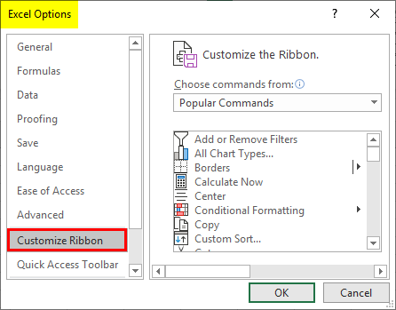
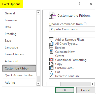
Step 1 – Right-click anywhere on the ribbon. It will open a pop-up with options, including “Customize the Ribbon.”
Step 2 – This will open the Excel Options box for you.
Step 3 – You can see two options on the screen: “Customize the Ribbon” on the right and the “Choose commands from” option on the left.

In the dropdown below, there are three options to customize the ribbon. By default, the “Main Tabs” is selected. The other two are “Tool Tabs” and “All Tabs.”
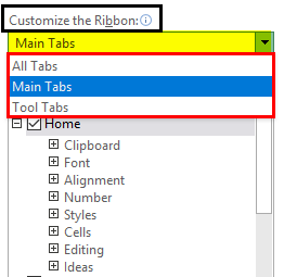
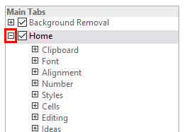
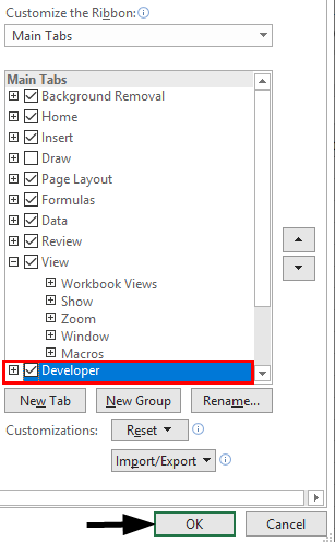
Step 4 – You can click on the (+) sign to expand the list.
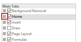
You will see some more tabs under the Main Tabs.

You can shrink the list by clicking on the (-) sign.
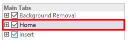
Step 5 – You can select or deselect the required tab to customize the ribbon. It will appear on the sheet accordingly.
You can also add additional tabs to your sheet by following the below steps.
- Click New Tab or New group and rename it with some name (not necessary) by clicking on the rename option.

- Go to choose a command from option and select the desired option from the dropdown.
- Add command to the tab or group you have created.

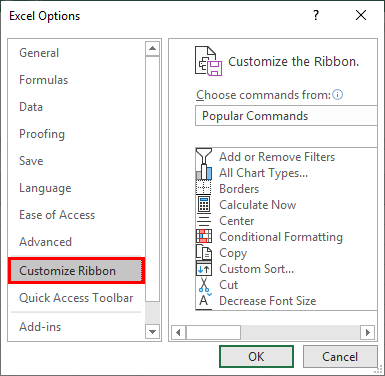
Note: You can also open the excel option pop-up by following steps.
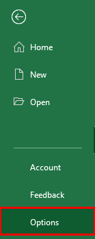
Click on File Menu —> Options
It will open Excel options for you, where you will see the option to customize the ribbon.
How to Collapse (Minimize) Ribbon in Excel?
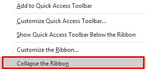
You can collapse the ribbon by right-clicking anywhere on the ribbon and then selecting the “Collapse the Ribbon” option.
How to Use a Ribbon in Excel with Examples
Below are some examples where you required customization of the ribbon.
Example #1
Someone asks you to record a macro or write a code in VBAVBA code refers to a set of instructions written by the user in the Visual Basic Applications programming language on a Visual Basic Editor (VBE) to perform a specific task.read more. How will you do that?
Solution:
We can use excel shortcutsAn Excel shortcut is a technique of performing a manual task in a quicker way.read more “Alt + F8” to record macro and “Alt + F11” to open the VBA screen. But remembering shortcuts is not always easy, so here is another option.
Shortcut key to Record Macro:
![]()
Shortcut key to Open VBA Screen:
![]()
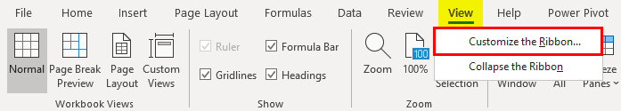
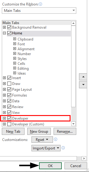
Add developer ribbon in excel by using the following steps. First, “Customize the Ribbon” will open the Excel options box.
Check on the developer option shown in the list under the main tabs. See the image below. Click Ok.

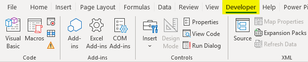
You will see the developer tabEnabling the developer tab in excel can help the user perform various functions for VBA, Macros and Add-ins like importing and exporting XML, designing forms, etc. This tab is disabled by default on excel; thus, the user needs to enable it first from the options menu.read more under your ribbon. See the image below.

You can see the macros or basic visual screens option.
Example #2
Someone asks you to create an interactive dashboard using Power View in ExcelExcel Power View is a data visualization technology that helps you create interactive visuals like graphs, charts. It allows you to analyze data by looking at the visuals you created. As a result, it makes your excel data more meaningful and insightful for better decision making.read more 2016 version.
Solution:
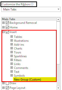
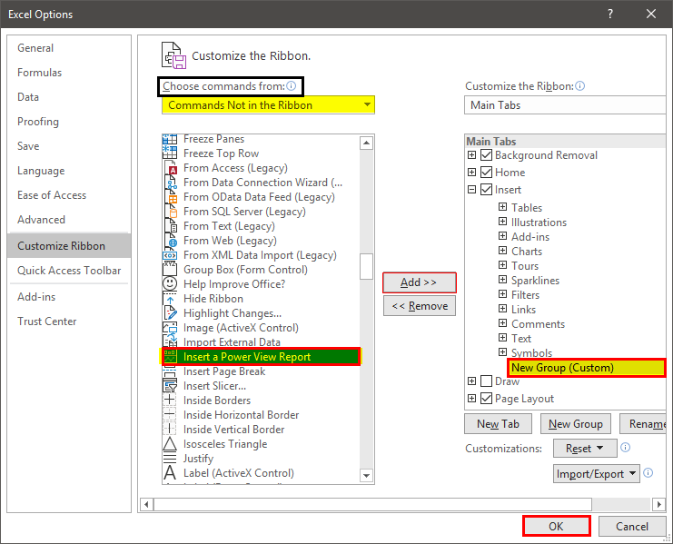
The “Power View” option is hidden in Excel 2016. So, we must follow the below steps to add the “Power View” command in our Excel. First, go to “Customize the Ribbon.”
Under “Customize the Ribbon,” extend the “Insert” option, then click on the “New Group (Custom).”
Now, choose the command shown on the left and select the command, not in the ribbon from the dropdown. Now, select “Insert a Power View Report.” Next, click on “Add.” It will add a “Power View” under the “Insert” tab. (When you click on “Add,” make sure a “New Group (Custom)” is selected. Else, an error will pop up). Select “OK.” See the below image:
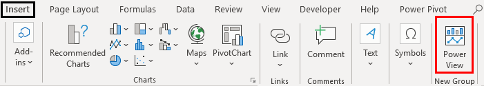
Now you can see the power view option under the insert tab in the new group section:
Example #3
Let’s take another scenario.
Suppose we are working on a report requiring the sum of the values in subsequent rows or columns very frequently.
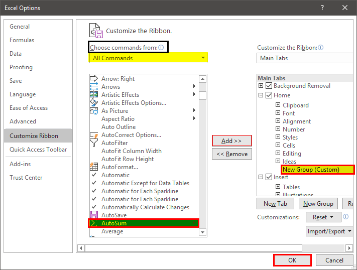
To sum up the values, we need to write a SUM function whenever the total value is required. Here, we can simplify our work by adding the AutoSum command to our ribbon. Then, go to “Customize the Ribbon.”
Under customize, the ribbon, Extend home, then click on the new group.
Now, choose the command shown on the left and select “All commands” from the dropdown. Now, select the “∑” AutoSum option. Next, click on “Add.” It will add “∑” “AutoSum” under the “Home” tab. (when you click on “Add,” make sure a “New Group (Custom)” is selected. Else, an error will pop up). Select “OK.” See the below image:
Now you can see the Autosum option under Home Tab in the New Group section:

Now let us see the use of it.
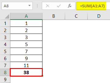
We have some numbers in cells A1 to A7. We need to get the sum in A8. Select cell A8 and click “AutoSum.” It will automatically apply the SUM formula for the active range and give you the SUM.
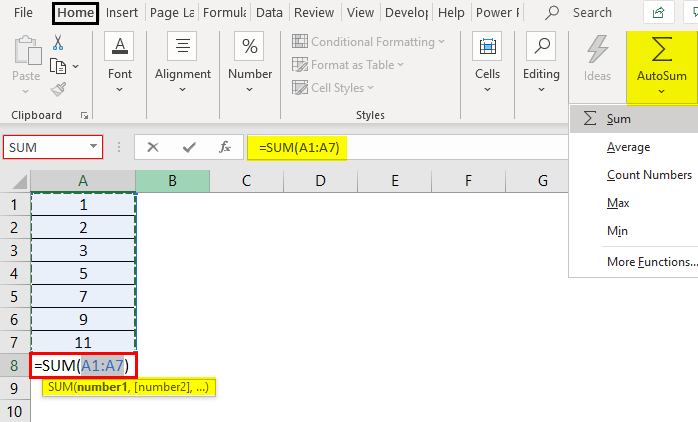
We get the following result.
Things to Remember
- We must slow the performance by adding tabs to the ribbon. So, we must add and keep only those tabs, whichever is required frequently.
- We must add a logical command to a logical group or tab so it can easily find that command.
- When adding commands from the “Command” option, not the ribbon, we must ensure that we have created a “New Group (Custom).” Otherwise, it will display the error.
Recommended Articles
This article is a guide to Ribbon in Excel. Here, we discuss how to customize, collapse, and use ribbon in Excel, along with examples and explanations. You can learn more about Excel from the following articles: –
- List of Top 10 Excel Commands
- Step Chart work in ExcelStep Chart in excel shows the exact time of change along with the trend of the data points as well.read more
- Watermark in Excel
- Excel 2016 RibbonsRibbons in Excel 2016 are designed to help you easily locate the command you want to use. Ribbons are organized into logical groups called Tabs, each of which has its own set of functions.read more
Содержание
- Show the ribbon
- Using the Ribbon Display Options
- Using the Ribbon Display Options
- Ribbon in Excel
- What is Ribbon in Excel?
- How to Customize Ribbon in Excel?
- How to Collapse (Minimize) Ribbon in Excel?
- How to Use a Ribbon in Excel with Examples
- Example #1
- Example #2
- Example #3
- Things to Remember
- Recommended Articles
- Command Ribbon
- What Is The Command Ribbon?
- What Tabs Are In The Ribbon?
- Selecting Commands From The Ribbon Using Keyboard Shortcuts
- Customizing The Ribbon
- Move Or Rename Tabs And Groups
- Remove Tabs Or Groups
- Add Custom Tabs And Groups
Show the ribbon
The Ribbon has multiple display options to fit your preferences, but with an errant click, you can unintentionally hide your Ribbon.
To quickly show the Ribbon, click any tab, for example, the Home or Insert tab.
To show the Ribbon all the time, click the arrow on the lower-right corner of the Ribbon.
For more control of the Ribbon, you can change your view and maximize the Ribbon by accessing the Ribbon Display Options near the top of your Excel document.
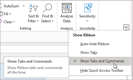
Using the Ribbon Display Options
Click the Ribbon Display Options button in the lower-right corner of the ribbon.
In the menu that opens, click Show Tabs and Commands to show the Ribbon with all tabs and full commands.
This option is the default view. While this option provides quick access to all the commands, it limits the available screen space for your workbook.
Tip: Press Ctrl+F1 to show and hide your commands in the Ribbon.
Click Show Tabs to display the Ribbon tabs without the commands. To access the commands in the Show Tabs option, click any of the tabs.
Click Auto-hide Ribbon to hide all tabs and commands.
By using this option, you get the largest amount of screen space when you view your workbook. To access tabs and commands in this view, click the very top of your workbook.
Tip: You can customize the Ribbon with your own tabs and commands for quick access to the toolbar features you use most.
The Ribbon has multiple display options to fit your preferences, but with an errant click, you can unintentionally hide your Ribbon.
To quickly show the Ribbon, click any tab, for example, the Home or Insert tab.
To show the Ribbon all the time, click the arrow (Excel 2013) or pushpin icon (Excel 2016) on the lower-right corner of the Ribbon.
For more control of the Ribbon, you can change your view and maximize the Ribbon by accessing the Ribbon Display Options near the top of your Excel document.
Using the Ribbon Display Options
Click the Ribbon Display Options icon on the top-right corner of your document. It is to the left of the Minimize icon.
In the menu that opens, click Show Tabs and Commands to show the Ribbon with all tabs and full commands.
This option is the default view. While this option provides quick access to all the commands, it limits the available screen space for your workbook.
Tip: Press Ctrl+F1 to show and hide your commands in the Ribbon.
Click Show Tabs to display the Ribbon tabs without the commands. To access the commands in the Show Tabs option, click any of the tabs.
Click Auto-hide Ribbon to hide all tabs and commands.
By using this option, you get the largest amount of screen space when you view your workbook. To access tabs and commands in this view, click the very top of your workbook.
Tip: You can customize the Ribbon with your own tabs and commands for quick access to the toolbar features you use most.
Источник
Ribbon in Excel


What is Ribbon in Excel?
The ribbon is an element of the UI (User Interface) at the top of Excel. In simple words, the ribbon can be called a strip consisting of buttons or tabs seen at the top of the Excel sheet. The ribbon was first introduced in Microsoft Excel in 2007.
In an earlier version of Excel, a menu and toolbar were replaced by a ribbon 2007. The basic tabs under the ribbon are – “Home,” “Insert,” “Page Layout,” “Formulas,” “Data,” “Review,” and “View.” We can customize it according to the requirements. See the image below. The highlighted strip is called ribbon, consisting of tabs like “Home, “Insert,” etc.
Table of contents
How to Customize Ribbon in Excel?
Below are the steps to customize the ribbon.
Step 1 – Right-click anywhere on the ribbon. It will open a pop-up with options, including “Customize the Ribbon.”
Step 2 – This will open the Excel Options box for you.
Step 3 – You can see two options on the screen: “Customize the Ribbon” on the right and the “Choose commands from” option on the left.
In the dropdown below, there are three options to customize the ribbon. By default, the “Main Tabs” is selected. The other two are “Tool Tabs” and “All Tabs.”
Step 4 – You can click on the (+) sign to expand the list.
You will see some more tabs under the Main Tabs.
You can shrink the list by clicking on the (-) sign.
Step 5 – You can select or deselect the required tab to customize the ribbon. It will appear on the sheet accordingly.
You can also add additional tabs to your sheet by following the below steps.
- Click New Tab or New group and rename it with some name (not necessary) by clicking on the rename option.

- Go to choose a command from option and select the desired option from the dropdown.
- Add command to the tab or group you have created.
Click on File Menu —> Options
It will open Excel options for you, where you will see the option to customize the ribbon.
How to Collapse (Minimize) Ribbon in Excel?
You can collapse the ribbon by right-clicking anywhere on the ribbon and then selecting the “Collapse the Ribbon” option.
How to Use a Ribbon in Excel with Examples
Below are some examples where you required customization of the ribbon.
Example #1
Solution:
We can use excel shortcuts Excel Shortcuts An Excel shortcut is a technique of performing a manual task in a quicker way. read more “Alt + F8” to record macro and “Alt + F11” to open the VBA screen. But remembering shortcuts is not always easy, so here is another option.
Shortcut key to Record Macro:

Shortcut key to Open VBA Screen:

Add developer ribbon in excel by using the following steps. First, “Customize the Ribbon” will open the Excel options box.
Check on the developer option shown in the list under the main tabs. See the image below. Click Ok.
You can see the macros or basic visual screens option.
Example #2
Solution:
The “Power View” option is hidden in Excel 2016. So, we must follow the below steps to add the “Power View” command in our Excel. First, go to “Customize the Ribbon.”
Under “Customize the Ribbon,” extend the “Insert” option, then click on the “New Group (Custom).”
Now, choose the command shown on the left and select the command, not in the ribbon from the dropdown. Now, select “Insert a Power View Report.” Next, click on “Add.” It will add a “Power View” under the “Insert” tab. (When you click on “Add,” make sure a “New Group (Custom)” is selected. Else, an error will pop up). Select “OK.” See the below image:
Now you can see the power view option under the insert tab in the new group section:
Example #3
Let’s take another scenario.
Suppose we are working on a report requiring the sum of the values in subsequent rows or columns very frequently.
To sum up the values, we need to write a SUM function whenever the total value is required. Here, we can simplify our work by adding the AutoSum command to our ribbon. Then, go to “Customize the Ribbon.”
Under customize, the ribbon, Extend home, then click on the new group.
Now, choose the command shown on the left and select “All commands” from the dropdown. Now, select the “∑” AutoSum option. Next, click on “Add.” It will add “∑” “AutoSum” under the “Home” tab. (when you click on “Add,” make sure a “New Group (Custom)” is selected. Else, an error will pop up). Select “OK.” See the below image:
Now you can see the Autosum option under Home Tab in the New Group section:
Now let us see the use of it.
We have some numbers in cells A1 to A7. We need to get the sum in A8. Select cell A8 and click “AutoSum.” It will automatically apply the SUM formula for the active range and give you the SUM.
We get the following result.
Things to Remember
- We must slow the performance by adding tabs to the ribbon. So, we must add and keep only those tabs, whichever is required frequently.
- We must add a logical command to a logical group or tab so it can easily find that command.
- When adding commands from the “Command” option, not the ribbon, we must ensure that we have created a “New Group (Custom).” Otherwise, it will display the error.
Recommended Articles
This article is a guide to Ribbon in Excel. Here, we discuss how to customize, collapse, and use ribbon in Excel, along with examples and explanations. You can learn more about Excel from the following articles: –
Источник
Command Ribbon
What Is The Command Ribbon?
The Ribbon is Excel’s command menu interface. It organizes commonly used actions together in an intuitive and visual way. These are the main parts of the Ribbon.
- Tabs organize related groups of commands together.
- Groups organize related commands together.
- Command Buttons allows you to perform actions or open menus with further related actions.
- Command Menu some command buttons will have a small down arrow located to the right or below the button. This indicates that a menu is available with sub-commands under the command button.
- Dialog Box certain groups in the ribbon will contain a small icon in the lower right hand corner that will launch a dialog box with further options available.
- Pin or Unpin Toggle allows you to remove the ribbon from view to create more workbook space.
What Tabs Are In The Ribbon?
There are 7 Tabs in Excel’s default setup.
- Home contains commands related to creating, formatting, and editing a spreadsheet.
- Insert contains commands related to adding items to a spreadsheet such as graphics, tables, pivot tables, charts, headers and footers, hyperlinks etc…
- Page Layout contains commands related to printing a spreadsheet.
- Fomulas contains commands related to adding and error checking formulas in a spreadsheet.
- Data contains commands related to importing and querying data in a spreadsheet.
- Review contains commands related to proof reading, commenting, protecting or tracking changes in the spreadsheet.
- View contains commands related to the display area of a spreadsheet.
In addition to these 7 Tabs, there is an 8th one called the Developer tab that is hidden by default. You can read this post to find out How To Enable The Developer Tab . The Developer tab contains commands related to recording macros and writing visual basic for application (VBA) code. This tab is hidden by default as most people will likely never want or need to use it.

Excel also has Contextual Tabs. These tabs only appear when a particular type of object is selected in the worksheet. For example, if we select a table object in our workbook, the Table Tools Design tab will appear which contains commands only related to tables.
Selecting Commands From The Ribbon Using Keyboard Shortcuts

Commands can be accessed in the regular way by using the mouse or by touch on touch screen devices, but they can also be accessed with keyboard shortcuts. To use any command in the ribbon with a keyboard shortcut, start by pressing the Alt key. This will display letters underneath the tabs that represent the next step in the shortcut. If we wanted to use a command in the Home tab we would press H next. Now each command in the ribbon will have a letter(s) or number next to it again representing the next step in the shortcut. If we wanted to perform the indent command, we would press 6 on the keyboard. Every command is accessible in this way, but some of the most used commands in Excel have much simpler keyboard shortcuts in addition to these. For Example, using this method to access the bold command results in Alt + H + 1, but it also has the much easier to execute and remember shortcut Ctrl + B.
Customizing The Ribbon
You can customize your Ribbon in a few different ways.
- Rearrange the order of tabs or groups within tabs or rename any tab or group.
- Remove groups from existing tabs or remove entire tabs from the ribbon.
- Add a custom group of commands of your choice to an existing tab in the ribbon.
- Add your own custom tabs with custom groups of commands of your choice. These can be commands that are already available in the default ribbon, but you can also add hidden commands that aren’t available in the default ribbon. This is great for creating a personalized menu of your most frequently used commands.
To customize the ribbon in any of these ways right click anywhere on the ribbon and select Customize the Ribbon from the menu.
Move Or Rename Tabs And Groups
Move Or Rename Tabs And Groups.
- Make sure you’re in the Customize Ribbon section of the Excel Options window.
- Select the Tab you want to move.
- Use the Up or Down arrows to move the tab.
- Select the Group you want to move and use the Up or Down arrows to move it.
- The Tab and/or Group should now appear in a different order in the Main Tabs box.
- Rename any Tab or Group by selecting it and either right click on it then choose Rename from the menu or press the Rename button.
- Change the display name and press the OK button.
- Press the OK button to implement all your changes.
Remove Tabs Or Groups
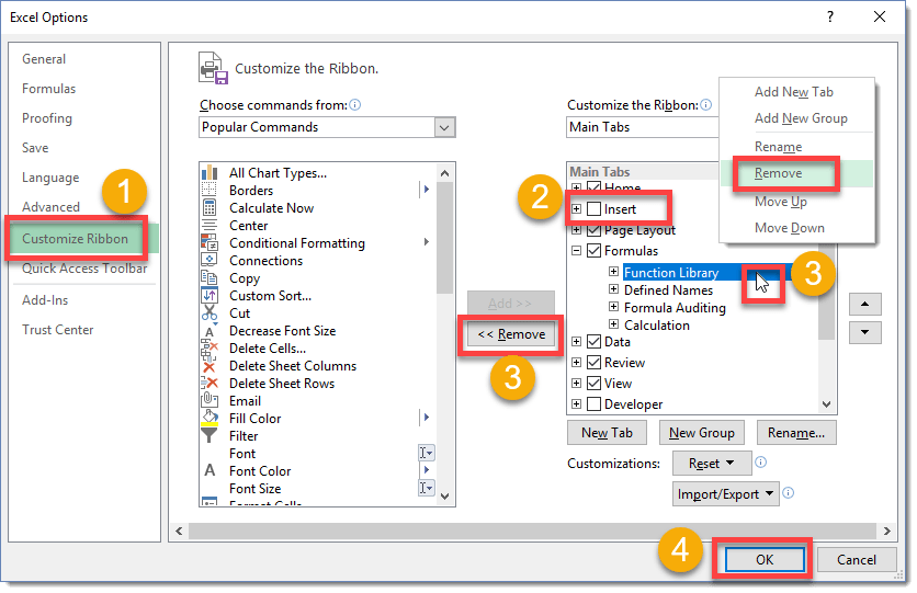
Remove Tabs or Groups from the Ribbon.
- Make sure you’re in the Customize Ribbon section of the Excel Options window.
- Remove a Tab from the Ribbon by unchecking it.
- Remove a Group from the Ribbon by selecting it then either right click and choose Remove from the menu or press the Remove button.
- Press the OK button to implement all your changes.
Add Custom Tabs And Groups
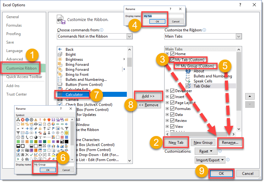
Add custom Tabs and Groups to the Ribbon.
- Make sure you’re in the Customize Ribbon section of the Excel Options window.
- Press the New Tab button to add a new Tab (Excel will add one Group to any new tab) or press the New Group button to add a new Group.
- Select your new tab and press the Rename button to give it a meaningful name.
- Change the display name and press the OK button.
- Repeat this with any new Groups. Select the Group and press the Rename button.
- Change the display name and press the OK button.
- You new Group will not have any commands, so you’ll need to add some. Select a command you want to add to your Group.
- Press the Add button to add it to your Group.
- Press the OK button to implement all your changes.
Источник
Excel Ribbon (Table of Contents)
- Components of Ribbon in Excel
- Examples of Ribbon in Excel
What is Excel Ribbon?
A ribbon or ribbon panel is the combination of all tabs except the File tab. The ribbon Panel shows the commands we need to complete a work. It is a part of the Excel Window. It contains several task-specific commands that are grouped under various command tabs. Additionally, the Ribbon panel provides instant access to the Excel help system, allowing us to search for information easily. The Ribbon Panel also provides screen tips. A descriptive text, also known as a screen tip, is displayed when we position the mouse pointer on a command in the Ribbon Panel.
There are four main elements in MS Excel.
- File Tab
- Quick Access Toolbar
- Ribbon
- Status Bar
- Formula Bar
- Task Pane
Components of Ribbon in Excel
The following tabs appear on the Ribbon Panel:
- Home
- Insert
- Page Layout
- Formulas
- Data
- Review
- View
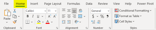
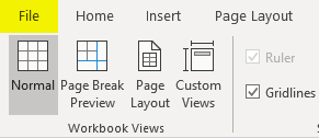
1. Home Tab
The Home tab helps perform clipboard operations, such as cut, copy, paste, and basic text and cell formatting. The Home tab includes the following groups:
- Clipboard
- Font
- Alignment
- Number
- Styles
- Cells
- Editing
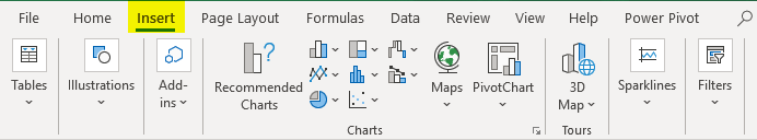
2. Insert Tab
The Insert tab helps us to insert objects such as a table, chart, illustrations, text, and hyperlinks in a worksheet. The Insert Tab includes the following groups:
- Tables
- Illustrations
- Apps
- Charts
- Report
- Sparklines
- Filters
- Links
- Text
- Symbols
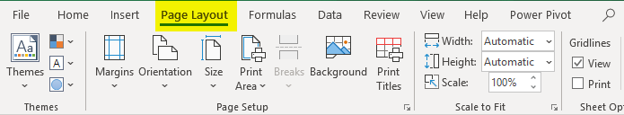
3. Page Layout Tab
The Page Layout tab helps us specify page settings, layout, orientation, margins, and other related options such as themes and gridlines. The Page Layout tab includes the following groups:
- Themes
- Page Setup
- Scale to Fit
- Sheet Options
- Arrange
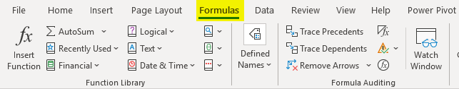
4. Formulas Tab
The Formula tab helps in working easily with formulas and functions. The Formula tab includes the following groups:
- Function Library
- Defined Names
- Formula Auditing
- Calculation
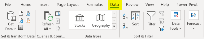
5. Data Tab
The Data tab helps in data-related tasks, such as setting up connections with external data sources and importing data for use within Excel worksheets. The Data tab includes the following groups:
- Get External Data
- Connections
- Sort & Filter
- Data Tools
- Outline
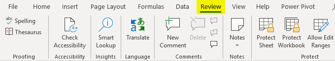
6. Review Tab
The Review tab helps in accessing tools that can be used for reviewing an Excel worksheet. It also enables you to insert comments, ensure that the language used in the worksheet is correct, and convert text to a different language, and share your workbook and worksheets.
The Review tab includes the following groups:
- Proofing
- Language
- Comments
- Changes
- Share
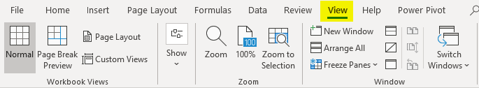
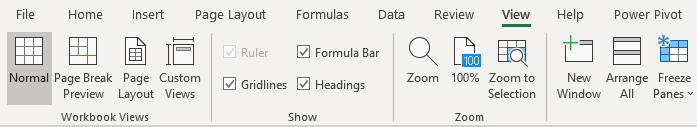
7. View Tab
The View tab allows you to view a worksheet in different views. In addition, it provides options to show or hide the elements of a worksheet window, Such as rulers or gridlines.
The View tab includes the following groups:
- Workbook Views
- Show
- Zoom
- Window
- Macros
Examples of Ribbon in Excel
Let’s understand how to use the Ribbon in Excel with some examples.
Example #1 – Add Developer Tab
There are 2 ways in which we can add the Developer tab.
Step 1: Right-click on Ribbon Panel.
Step 2: Click on the ‘Customize the Ribbon’ option
Step 3: A dialog box named ‘Excel options’ will appear, and click on the ‘Customize Ribbon’ menu option.
Step 4: On the right pane, select the Developer Tab and Click on the OK check-in box.
Step 5: The developer tab will appear in the Ribbon Panel.
Step 6: Click on the File tab.
Step 7: A backstage view will appear. Click on Options.
Step 8: A dialog box named ‘Excel Options’ will appear.
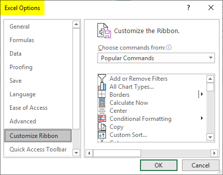
Step 9: Click on the ‘Customize Ribbon’ menu option.
Step 10: On the right pane, select the check-in box of the Developer tab and click on OK.
Step 11: The developer tab will appear in the Ribbon Panel.
Example #2 – Remove Developer Tab
There are 2 two ways in which we can add the Developer tab:
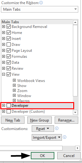
Step 1: Right-click on Ribbon Panel and click on the ‘Customize the Ribbon’ option.
Step 2: A dialog box named ‘Excel options’ will appear.
Step 3: Click on the ‘Customize Ribbon’ menu option.
Step 4: On the right pane, deselect the check-in box of the Developer tab and click on OK.
Step 5: The developer tab will disappear from the Ribbon Panel.
Step 6: Click on File Tab.
Step 7: A backstage view will appear. Click on Options.
Step 8: A dialog box named ‘Excel options’ will appear.
Step 9: Click on the ‘Customize Ribbon’ menu option.
Step 10: On the right pane, deselect the check-in box of the Developer Tab and click on OK.
Step 11: The developer tab will disappear in the Ribbon Panel.
Example #3 – Add Customized Tab
We can add a customized tab by using the following steps:
Step 1: Click on File Tab.
Step 2: A backstage view will appear. Click on Options.
Step 3: A dialog box named ‘Excel Options’ will appear.
Step 4: Click on the ‘Customize Ribbon’ menu option.
Step 5: Under the right pane, click on New Tab to create a new tab in Ribbon.
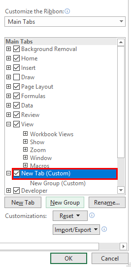
Step 6: We can rename the tab by clicking on the Rename option.
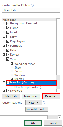
Step 7: We can also create a partition in the Tab by Clicking on the New Group option.
Step 8: We can add the command to different groups by clicking on them on the right pane.
Step 9: We can choose the commands from the list in the left pane.
Step 10: Click on Add.
Step 11: On the right pane, select the new Tab and Click on the OK check-in box.
Step 12: The New Tab will appear in the Ribbon Panel.
Things to Remember
- We need to remember the flow. Tab Group Aa.
- Any Information needed on Ribbon, just press F1 (Help).
Recommended Articles
This is a guide to Ribbon in Excel. Here we discuss How to use Ribbon in Excel along with practical examples and a downloadable excel template. You can also go through our other suggested articles –
- VLOOKUP Examples in Excel
- Excel Developer Tab
- Excel Repair
- Add Rows in Excel Shortcut
![]()
Excel Ribbon

Excel ribbon is the navigation menu in Excel, shows all the Controls and Commands in different Tabs. All commands available in Excel are grouped and provided in separate tabs of Ribbon based on the functionality to deal with verity of the Objects in Excel.
There are several Tabs in Excel: File, Home, Insert, Draw, Page Layout, Data, Review, View, Developer, Add-ins, Help,etc. You can see the built-in command bars are grouped together in each ribbon based on its functionality.
- Components of the Excel Ribbon:
- List of Tabs in Ribbon
- Commands in Ribbon:
- Home Tab:
- Insert Tab:
- Page Layout Tab:
- Formulas Tab:
- Data Tab:
- Review Tab:
- View Tab:
- Developer Tab:
- Format Tab:
- Chart Tools Tab:
- PivotTable Tools Tab:
- PivotTable Design Tab:
- Shape Format Tab:
- Add-ins Tab:
- Frequently Asked Questions and Answers
Components of the Excel Ribbon:
Excel Ribbon Can be divided into several Parts. Here are the Different parts of the Excel Ribbon.
- BackView: BackView Of the Excel Ribbon Contains File Information, Open, New, Save, Export and Options.
- Quick Access Toolbar: Top Left Conner of The Excel Ribbon Contains Quick Access Toolbar. You can add any command to this Ribbon Part to quickly access the command bars.
- Ribbon Tabs: Excel Ribbon Contains Ribbon Tabs to show the Excel Commands. Excel is grouped all the commands into these ribbon for easy access.
- Groups: All the similar commands are grouped into one group in each Tab. Every Excel Ribbon Tab contains one or multiple Groups
List of Tabs in Ribbon
Here are the list of Tabs available in Excel Ribbon Menu. Each tab contains verity of Excel commands divided into different groups in Excel Ribbon Tabs.
- File Tab: All the commands related to Excel File to Save, Open, Close and Change the Excel Options
- Home Tab: Home Tab contains the standard Excel Commands. Most of these are related to Formatting and Copy Paste Commands. For Example: Copy, Cut, Paste, Font, Bold, Alignment, Number Formatting, Insert, Delete, etc.
- Insert Tab: Insert Tab contains the commands to insert into Excel File. You can insert Table, Pivot Table, Picture, Shapes, Icons, Charts and Symbols.
- Draw Tab: This is newly added tab which provided with drawing tools.
- Page Layout Tab: All the commands related to Page settings and Layouts, Printing Options can view in Page Layout tab.
- Formulas Tab: You can view Excel Functions Library and Defined Names, Auditing and Calculations commands in Formulas Ribbon Tab.
- Data Tab: Data Tab contains commands for connecting and importing Data, Sorting and Filtering Data Commands, Data Validation, Text to Columns, Remove Duplicates and Outline commands.
- Review Tab: It contains Spell check, comments and protection commands.
- View Tab: You can view Workbook Views, Show, Zoom, Window and Macros from View Tab.
- Developer Tab: All the Commands related Excel VBA Development can be found in the Developer Tab.
- Format Tab: This tab contains commands for formatting cells, such as changing font size, color, and style, as well as border styles, shading, and cell protection.
- Chart Tools Tab: This tab is displayed when a chart is selected, and contains commands for customizing the appearance and data of the chart, such as adding or removing chart elements, changing chart types, and formatting chart data series.
- PivotTable Tools Tab: This tab is displayed when a PivotTable or PivotChart is selected, and contains commands for managing and analyzing large sets of data, such as creating calculated fields, grouping data, and filtering results.
- Add-ins Tab: This tab is displayed when a compatible add-in is installed and activated, and contains commands for working with the add-in’s features and functionality.
Overall, the Excel Ribbon provides users with a powerful and flexible interface for performing a wide variety of tasks, and its menus and commands can be customized to suit the specific needs and preferences of individual users.
Commands in Ribbon:
Here is a more detailed explanation of the common commands found in each of the tabs in the Excel Ribbon:
Home Tab:
- Clipboard: Cut, Copy, and Paste commands for moving or duplicating data within a worksheet or between different worksheets or workbooks.
- Font: Commands for formatting text, such as font style, size, color, bold, italic, underline, and strikethrough.
- Alignment: Commands for adjusting the alignment of text within cells, such as horizontal and vertical alignment, text wrap, and indent.
- Number: Commands for formatting numeric values, such as currency, date and time, percentage, and scientific notation.
- Styles: Commands for applying predefined styles to cells, such as Title, Heading, and Total styles.
- Cells: Commands for managing cells, such as inserting or deleting cells, hiding or unhiding rows and columns, and merging cells.
- Editing: Commands for editing data within cells, such as Find and Replace, Clear, and Undo and Redo.
| Group | Command | Description |
|---|---|---|
| Clipboard | Cut | Cut the selected cells, rows, or columns |
| Clipboard | Copy | Copy the selected cells, rows, or columns |
| Clipboard | Paste | Paste the copied or cut cells, rows, or columns |
| Clipboard | Paste Special | Choose a paste option, such as values or formatting |
| Clipboard | Format Painter | Copy the formatting of selected cells and apply it to other cells |
| Font | Font | Choose a font for the selected cells |
| Font | Font Size | Choose a font size for the selected cells |
| Font | Bold | Make the selected text bold |
| Font | Italic | Make the selected text italic |
| Font | Underline | Underline the selected text |
| Font | Strikethrough | Add a strikethrough to the selected text |
| Font | Subscript | Make the selected text a subscript |
| Font | Superscript | Make the selected text a superscript |
| Font | Change Case | Change the case of the selected text |
| Font | Text Effects | Add an effect, such as shadow or reflection, to the selected text |
| Font | Font Color | Choose a font color for the selected cells |
| Font | Fill Color | Choose a fill color for the selected cells |
| Alignment | Wrap Text | Wrap text within a cell |
| Alignment | Merge & Center | Merge selected cells and center the content |
| Alignment | Merge Across | Merge selected cells across a row |
| Alignment | Merge Cells | Merge selected cells |
| Alignment | Align Left | Align text to the left of the cell |
| Alignment | Center | Center text within a cell |
| Alignment | Align Right | Align text to the right of the cell |
| Alignment | Increase Indent | Increase the indentation of the text within a cell |
| Alignment | Decrease Indent | Decrease the indentation of the text within a cell |
| Alignment | Orientation | Change the orientation of the text within a cell |
| Alignment | Vertical Alignment | Choose a vertical alignment for the content within a cell |
| Number | Number Format | Choose a number format for the selected cells |
| Number | Percent Style | Apply a percent format to the selected cells |
| Number | Comma Style | Apply a comma format to the selected cells |
| Number | Increase Decimal | Increase the number of decimal places displayed for the selected cells |
| Number | Decrease Decimal | Decrease the number of decimal places displayed for the selected cells |
| Number | Accounting Number Format | Apply an accounting number format to the selected cells |
| Styles | Cell Styles | Apply a predefined cell style to the selected cells |
| Styles | Conditional Formatting | Apply formatting based on certain conditions |
| Cells | Insert | Insert cells, rows, columns, or sheets |
| Cells | Delete | Delete cells, rows, columns, or sheets |
| Cells | Format | Choose a cell format for the selected cells |
| Cells | Hide & Unhide | Hide or unhide rows, columns, or sheets |
| Cells | Find & Select | Find and select specific content within the worksheet |
| Editing | Find | Find specific content within the worksheet |
| Editing | Replace | Replace specific content within the worksheet |
| Editing | Go To | Go to a specific cell, row, column, or sheet |
| Editing | Sort & Filter | Sort or filter the data within the worksheet |
| Editing | Conditional Formatting | Apply formatting based on certain conditions |
| Editing | Clear | Clear the content or formatting of the selected cells |
| Editing | Data Validation | Set rules for the data entered in the |
Insert Tab:
- Tables: Commands for creating and formatting tables, such as Table, PivotTable, and Recommended Charts.
- Illustrations: Commands for inserting images, shapes, SmartArt, and charts.
- Add-ins: Commands for adding custom add-ins or features to Excel, such as My Add-ins, Store, and Office Add-ins.
- Charts: Commands for creating and formatting charts, such as Column, Line, Pie, and Scatter charts.
- Sparklines: Commands for creating and formatting small charts that fit within a single cell, such as Line, Column, and Win/Loss sparklines.
- Filter: Commands for filtering data within a table or range, such as Sort and Filter.
| Group | Command | Description |
|---|---|---|
| Tables | Table | Convert a range of cells into a table |
| Tables | PivotTable | Create a PivotTable from the selected data |
| Tables | Recommended Charts | View suggested chart types based on the selected data |
| Illustrations | Pictures | Insert a picture from a file or online source |
| Illustrations | Online Pictures | Search for and insert pictures from online sources |
| Illustrations | Shapes | Insert a shape, such as a line, rectangle, or arrow |
| Illustrations | Icons | Insert an icon from a library of built-in icons |
| Illustrations | 3D Models | Insert a 3D model from an online source or a file |
| Illustrations | SmartArt | Insert a SmartArt graphic, such as a process or hierarchy diagram |
| Illustrations | Chart | Insert a chart based on the selected data |
| Add-Ins | Add-Ins | View and manage available add-ins |
| Add-Ins | Store | Browse and download add-ins from the Microsoft Store |
| Charts | Column | Insert a column chart based on the selected data |
| Charts | Line | Insert a line chart based on the selected data |
| Charts | Pie | Insert a pie chart based on the selected data |
| Charts | Bar | Insert a bar chart based on the selected data |
| Charts | Area | Insert an area chart based on the selected data |
| Charts | Scatter | Insert a scatter chart based on the selected data |
| Charts | Map | Insert a map chart based on geographic data |
| Sparklines | Line | Insert a line sparkline to show trends within the selected data |
| Sparklines | Column | Insert a column sparkline to show trends within the selected data |
| Sparklines | Win/Loss | Insert a win/loss sparkline to show trends within the selected data |
| Filters | Filter | Add a filter to the selected data to allow for sorting and filtering |
| Text | Text Box | Insert a text box to add text or captions to the worksheet |
| Text | Header & Footer | Add headers and footers to the worksheet for printing |
| Text | WordArt | Insert stylized text to the worksheet |
| Text | Drop Cap | Add a decorative initial letter to the beginning of a block of text |
| Symbols | Symbol | Insert a symbol, such as a currency or mathematical symbol |
| Media | Audio | Insert an audio clip into the worksheet |
| Media | Video | Insert a video clip into the worksheet |
| Links | Hyperlink | Insert a hyperlink to another location or file |
| Links | Bookmark | Create a bookmark to a specific location within the worksheet |
| Comments | Comment | Add a comment to a cell to provide additional information |
| Other | Object | Insert an object, such as a file or chart, into the worksheet |
| Other | Equation | Insert an equation into the worksheet |
| Other | Signature Line | Insert a signature line for digital signatures |
Page Layout Tab:
- Themes: Commands for applying or customizing themes that change the overall appearance of a worksheet or workbook, such as colors, fonts, and effects.
- Page Setup: Commands for adjusting the page layout of a worksheet, such as margins, orientation, size, and print area.
- Scale to Fit: Commands for adjusting the scale of a worksheet to fit a certain number of pages, such as adjusting the width or height of printed pages.
- Sheet Options: Commands for adding or removing gridlines, headers, and footers, as well as controlling the visibility of objects such as shapes and charts.
- Arrange: Commands for arranging or aligning objects within a worksheet, such as Bring to Front, Send to Back, and Align Left.
| Group | Command | Description |
|---|---|---|
| Themes | Themes | Apply a predefined color scheme and font style to the worksheet |
| Themes | Colors | Apply a specific color scheme to the worksheet |
| Themes | Fonts | Apply a specific font style to the worksheet |
| Page Setup | Page Setup | Set up the page orientation, margins, and paper size for printing |
| Page Setup | Scale to Fit | Adjust the scaling of the worksheet to fit on a specific number of pages |
| Page Setup | Sheet Options | Set options for printing the worksheet, such as gridlines and headings |
| Page Setup | Arrange | Adjust the placement and order of objects, such as pictures and shapes |
| Page Setup | Background | Add a background image or color to the worksheet |
| Page Setup | Print Titles | Set rows and columns to repeat on each printed page |
| Page Setup | Page Borders | Add a border to the edges of the printed page |
| Page Setup | Watermark | Add a watermark, such as “Draft” or “Confidential,” to the worksheet |
| Page Setup | Breaks | Insert page breaks to control where pages end and new ones begin |
| Page Setup | View | Switch between different views, such as Normal and Page Break Preview |
| Page Setup | Macros | Record or run macros to automate tasks |
| Scale to Fit | Width | Adjust the scaling of the worksheet to fit on a specific number of pages horizontally |
| Scale to Fit | Height | Adjust the scaling of the worksheet to fit on a specific number of pages vertically |
| Scale to Fit | Scale | Adjust the scaling of the worksheet to fit on a specific number of pages both horizontally and vertically |
| Sheet Options | Gridlines | Show or hide gridlines on the printed worksheet |
| Sheet Options | Headings | Show or hide row and column headings on the printed worksheet |
| Sheet Options | Breaks | Show or hide page breaks on the printed worksheet |
| Sheet Options | Background | Show or hide the background image or color on the printed worksheet |
| Sheet Options | Draft Quality | Print the worksheet in draft quality to save ink and toner |
| Arrange | Position | Align objects to specific positions, such as center or left |
| Arrange | Size | Resize objects to specific dimensions |
| Arrange | Wrap Text | Wrap text around objects to fit them into the worksheet |
| Arrange | Bring Forward | Bring an object to the front of the worksheet |
| Arrange | Send Backward | Send an object to the back of the worksheet |
| Arrange | Group | Group multiple objects together for easier editing and formatting |
| Arrange | Rotate | Rotate an object to a specific angle |
| Macros | Macros | Record or run macros to automate tasks |
Formulas Tab:
- Function Library: Commands for inserting and working with built-in Excel functions, such as SUM, AVERAGE, and IF.
- Defined Names: Commands for creating and managing named ranges and formulas.
- Formula Auditing: Commands for tracing and evaluating formulas, such as Trace Precedents, Trace Dependents, and Evaluate Formula.
- Calculation: Commands for controlling the calculation settings of Excel, such as Automatic or Manual calculation, and Data Tables.
- Formula Bar: Commands for adjusting the display and editing of the Formula Bar, such as Show Formula or Show Functions.
| Group | Command | Description |
|---|---|---|
| Function Library | Insert Function | Open the Insert Function dialog box to search and select a specific function |
| Function Library | Financial | Perform financial calculations, such as calculating loan payments or depreciation |
| Function Library | Logical | Evaluate logical statements, such as IF statements |
| Function Library | Text | Manipulate text strings, such as concatenating or extracting specific characters |
| Function Library | Date & Time | Work with dates and times, such as calculating the difference between two dates |
| Function Library | Lookup & Reference | Look up and reference specific data in a worksheet or external file |
| Function Library | Math & Trig | Perform mathematical and trigonometric calculations, such as calculating the square root or sine of an angle |
| Function Library | More Functions | Open a list of additional functions, such as database and engineering functions |
| Defined Names | Define Name | Create a name for a cell or range of cells to make it easier to reference |
| Defined Names | Name Manager | Manage existing names, including renaming, deleting, and modifying |
| Formula Auditing | Trace Precedents | Show the cells that provide input to the selected cell |
| Formula Auditing | Trace Dependents | Show the cells that depend on the selected cell |
| Formula Auditing | Remove Arrows | Remove all tracing arrows |
| Formula Auditing | Error Checking | Check for errors in the worksheet formulas |
| Formula Auditing | Evaluate Formula | Evaluate the selected formula step by step |
| Calculation | Calculation Options | Change the calculation options, such as automatic or manual |
| Calculation | Calculate Now | Calculate all formulas in the worksheet |
| Calculation | Calculate Sheet | Calculate all formulas in the active worksheet |
| Calculation | Calculate Workbook | Calculate all formulas in the entire workbook |
| Calculation | Calculate Selection | Calculate only the selected cells |
| Calculation | Circular References | Display or ignore circular references |
| Calculation | Error Checking | Check for errors in the worksheet formulas |
| Calculation | Enable Iterative Calculation | Enable iterative calculation to solve circular references |
| Calculation | Watch Window | Add or remove cells to the watch window to monitor their values |
| Calculation | Evaluate Formula | Evaluate the selected formula step by step |
Data Tab:
- Get & Transform Data: Commands for importing and transforming data from external sources, such as Query Editor, Data Model, and From Other Sources.
- Sort & Filter: Commands for sorting and filtering data within a table or range, such as Sort A-Z, Sort Z-A, and Filter by Color.
- Data Tools: Commands for working with data, such as Data Validation, Remove Duplicates, and Text to Columns.
- Outline: Commands for creating and manipulating outlines of data, such as Group and Ungroup, and Subtotal.
- What-If Analysis: Commands for analyzing data under different scenarios, such as Goal Seek, Data Tables, and Scenario Manager.
| Group | Command | Description |
|---|---|---|
| Get & Transform Data | Get Data | Open the Get Data dialog box to import data from a variety of sources |
| Get & Transform Data | From Table/Range | Import data from a selected table or range |
| Get & Transform Data | From Table/Range (Power Query) | Import data from a selected table or range using Power Query |
| Get & Transform Data | Recent Sources | View and select recently used data sources |
| Get & Transform Data | Show Queries | View and manage all queries created using Power Query |
| Get & Transform Data | New Query | Create a new query using Power Query |
| Get & Transform Data | Combine Queries | Combine multiple queries into one |
| Get & Transform Data | Append Queries | Append two or more queries together |
| Get & Transform Data | Merge Queries | Merge two or more queries based on a common column |
| Get & Transform Data | Group By | Group rows together based on a selected column |
| Get & Transform Data | Pivot Column | Pivot a selected column to create a new table |
| Get & Transform Data | Unpivot Columns | Unpivot selected columns to create a new table |
| Get & Transform Data | Transform Data | Open the Power Query Editor to transform data |
| Connections | Existing Connections | View and manage existing connections to external data sources |
| Connections | Refresh All | Refresh all connections in the workbook |
| Connections | Edit Links | Edit links to external data sources |
| Sort & Filter | Sort A to Z | Sort the selected range in ascending order |
| Sort & Filter | Sort Z to A | Sort the selected range in descending order |
| Sort & Filter | Sort Smallest to Largest | Sort the selected range in ascending order, based on the values in the leftmost column |
| Sort & Filter | Sort Largest to Smallest | Sort the selected range in descending order, based on the values in the leftmost column |
| Sort & Filter | Custom Sort | Sort the selected range using custom sort criteria |
| Sort & Filter | Filter | Add a filter to the selected range |
| Sort & Filter | Clear | Clear any existing filters |
| Sort & Filter | Advanced | Open the Advanced Filter dialog box to create more complex filters |
| Data Tools | Remove Duplicates | Remove duplicate values from the selected range |
| Data Tools | Data Validation | Add data validation rules to the selected cells |
| Data Tools | What-If Analysis | Perform what-if analysis using scenarios, goal seek, or data tables |
| Outline | Group | Group selected rows or columns together |
| Outline | Ungroup | Remove groupings from selected rows or columns |
| Outline | Subtotal | Add subtotals to the selected range |
| Outline | Show Detail | Show all detail rows within a grouped range |
| Outline | Hide Detail | Hide all detail rows within a grouped range |
| Outline | Create from Selection | Create a new group from a selected range |
Review Tab:
- Proofing: Commands for checking the spelling and grammar of text within a worksheet, as well as adding and managing custom dictionaries.
- Comments: Commands for adding, viewing, and managing comments within a worksheet, as well as controlling the display and formatting of comments.
- Changes: Commands for tracking and managing changes made to a worksheet, such as accepting or rejecting changes, and comparing different versions of a workbook.
- Compare: Commands for comparing and merging different versions of a workbook or worksheet.
- Protect: Commands for protecting a worksheet or workbook, such as password-protecting cells, or restricting access to certain users or groups.
| Group | Command | Description |
|---|---|---|
| Proofing | Spelling | Check the spelling of the selected text or the entire worksheet |
| Proofing | Research | Open the Research task pane to search for information |
| Proofing | Thesaurus | Open the Thesaurus task pane to find synonyms and antonyms |
| Proofing | Translate | Translate selected text or entire worksheet to another language |
| Proofing | Word Count | Count the number of words, characters, and paragraphs in the selected text or the entire worksheet |
| Comments | New Comment | Add a new comment to the selected cell |
| Comments | Edit Comment | Edit the selected comment |
| Comments | Delete | Delete the selected comment |
| Comments | Previous | Navigate to the previous comment |
| Comments | Next | Navigate to the next comment |
| Changes | Protect Sheet | Protect the worksheet and specify which cells can be edited |
| Changes | Allow Users to Edit Ranges | Specify which ranges can be edited by which users |
| Changes | Protect Workbook | Protect the workbook with a password and specify which elements can be edited |
| Changes | Share Workbook | Allow multiple users to edit the workbook simultaneously |
| Changes | Track Changes | Track changes made to the workbook |
| Changes | Highlight Changes | Highlight changes made to the workbook |
| Changes | Accept/Reject Changes | Accept or reject changes made to the workbook |
| Changes | Protect and Share Workbook | Protect the workbook and share it with others |
| Changes | Protect and Share Workbook with Excel Online | Protect the workbook and share it with others using Excel Online |
| Changes | Compare and Merge Workbooks | Compare and merge changes made to two different versions of the same workbook |
| Changes | Merge Workbooks | Combine multiple workbooks into one |
| Changes | Workbook Version History | View the version history of the workbook |
| Changes | Restore | Restore the workbook to a previous version |
| Changes | Open Version | Open a previous version of the workbook |
| Changes | Delete All Comments | Delete all comments in the workbook |
| Changes | Delete Comment | Delete the selected comment |
| Changes | Show All Comments | Show all comments in the worksheet |
| Changes | Show/Hide Markup | Show or hide changes and comments made to the workbook |
| Changes | Protect and Share Workbook with SharePoint | Protect the workbook and share it with others using SharePoint |
| Changes | Protect and Share Workbook with OneDrive | Protect the workbook and share it with others using OneDrive |
| Changes | Protect and Share Workbook with OneDrive for Business | Protect the workbook and share it with others using OneDrive for Business |
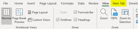
View Tab:
- Workbook Views: Commands for changing the view of a workbook, such as Normal, Page Layout, and Page Break Preview.
- Show: Commands for displaying or hiding certain elements within a worksheet, such as Gridlines, Headings, and Formula Bar.
- Zoom: Commands for adjusting the zoom level of a worksheet, such as Zoom In or Zoom Out, and Fit to Window.
- Window: Commands for managing multiple windows or views of a workbook, such as Split, Freeze Panes, and New Window.
- Macros: Commands for recording or editing macros within a workbook, as well as managing the security and settings for macros.
| Group | Command | Description |
|---|---|---|
| Workbook Views | Normal | Display the worksheet in Normal view |
| Workbook Views | Page Layout | Display the worksheet in Page Layout view |
| Workbook Views | Page Break Preview | Display the worksheet in Page Break Preview view |
| Workbook Views | Custom Views | Create, modify, or delete custom views of the worksheet |
| Workbook Views | Full Screen | Display the worksheet in Full Screen view |
| Workbook Views | Switch Windows | Switch between open workbooks |
| Show | Gridlines | Show or hide gridlines |
| Show | Headings | Show or hide row and column headings |
| Show | Formula Bar | Show or hide the Formula Bar |
| Show | Ruler | Show or hide the ruler |
| Show | Zoom | Change the zoom level of the worksheet |
| Show | Arrange All | Arrange all open workbooks |
| Show | New Window | Create a new window for the current workbook |
| Show | Freeze Panes | Freeze the selected rows or columns |
| Show | Split | Split the worksheet into multiple panes |
| Show | Window | Display the Window menu |
| Macros | Macros | Display the Macros dialog box to create, edit, or delete macros |
| Macros | Record Macro | Record a new macro |
| Macros | Use Relative References | Toggle the use of relative references in recorded macros |
| Macros | Stop Recording | Stop recording the macro |
| Macros | Macros Security | Set the level of security for running macros |
| Workbook Views | View Side by Side | View two workbooks side by side |
| Workbook Views | Synchronous Scrolling | Synchronize scrolling between two worksheets |
| Workbook Views | Reset Window Position | Reset the position of the active workbook window |
| Workbook Views | View Code | Display the Visual Basic Editor |
| Workbook Views | Macros | View the list of macros in the current workbook |
| Workbook Views | Zoom to Selection | Zoom in on the selected cell or range |
| Workbook Views | Full Screen | Display the worksheet in Full Screen view |
Developer Tab:
- Code: Commands for creating, editing, and running macros and code within Excel, such as Visual Basic Editor, Macros, and Code Snippets.
- Add-ins: Commands for working with add-ins and controls within Excel, such as ActiveX Controls, Add-ins, and XML.
- Controls: Commands for inserting, customizing, and working with form controls, such as Buttons, Check Boxes, and Drop-Down Lists.
- XML: Commands for working with XML data within Excel, such as XML Mapping, Import, and Export.
| Group | Command | Description |
|---|---|---|
| Code | Visual Basic | Open the Visual Basic Editor |
| Code | Macros | Display the Macros dialog box to create, edit, or delete macros |
| Code | Record Macro | Record a new macro |
| Code | Use Relative References | Toggle the use of relative references in recorded macros |
| Code | Stop Recording | Stop recording the macro |
| Code | Macros Security | Set the level of security for running macros |
| Add-Ins | Excel Add-Ins | Manage Excel Add-Ins |
| Controls | Insert | Insert form controls such as buttons, checkboxes, and drop-down lists |
| Controls | Design Mode | Toggle design mode for form controls |
| Controls | Properties | Display the Properties dialog box for a selected form control |
| XML | Source | Display the XML source code for the current workbook |
| XML | Show XML Tools | Display the XML Tools menu |
| XML | Map Properties | Display the Map Properties dialog box for the current XML map |
| XML | Export | Export the XML data to an XML file or other format |
| XML | Import | Import XML data into the current worksheet |
| XML | Refresh Data | Refresh the XML data in the worksheet |
| XML | Clear Map | Remove the XML mapping from the worksheet |
| Add-Ins | Add-Ins | Display the Add-Ins dialog box |
| Code | Macro Security | Set the level of security for running macros and add-ins |
| Code | Visual Basic | Open the Visual Basic Editor |
Format Tab:
- Cells: Commands for formatting cells, such as Cell Styles, Format Cells, and Conditional Formatting.
- Font: Commands for formatting text within cells, such as Font Styles, Size, and Effects.
- Alignment: Commands for aligning text and objects within cells, such as Horizontal and Vertical Alignment, Indentation, and Orientation.
- Number: Commands for formatting numbers and dates within cells, such as Number Formats, Currency, and Percentage.
- Styles: Commands for applying, creating, or modifying cell styles within a worksheet.
| Group | Command | Description |
|---|---|---|
| Cells | Format Cells | Opens the Format Cells dialog box where you can format various cell properties |
| Merge & Center | Combines selected cells and centers the content horizontally | |
| Wrap Text | Wraps text within a cell to fit the width of the cell | |
| Freeze Panes | Keeps rows and/or columns visible while scrolling through a worksheet | |
| Font | Font | Changes the font face, size, color, and other font attributes |
| Bold | Makes text bold | |
| Italic | Makes text italic | |
| Underline | Underlines text | |
| Alignment | Align Left | Aligns text to the left |
| Center | Centers text horizontally | |
| Align Right | Aligns text to the right | |
| Top | Aligns text to the top | |
| Middle | Centers text vertically | |
| Bottom | Aligns text to the bottom | |
| Borders | Border | Adds or removes cell borders |
| Color | Changes the color of cell borders | |
| Line Style | Changes the line style of cell borders | |
| Border Styles | Applies a predefined border style to selected cells | |
| Fill | Fill Color | Changes the background color of cells |
| Pattern Fill | Fills cells with a pattern or texture | |
| Gradient Fill | Fills cells with a gradient | |
| Cell Styles | Cell Styles | Applies predefined cell styles |
| New Cell Style | Creates a new cell style based on selected cells | |
| Conditional | Highlight | Highlights cells based on certain conditions |
| Formatting | Clear | Clears cell formatting |
Chart Tools Tab:
- Design: Commands for designing the appearance and layout of a chart, such as Chart Styles, Chart Layouts, and Chart Titles.
- Data: Commands for managing the data source and values of a chart, such as Select Data, Switch Row/Column, and Edit Data.
- Layout: Commands for customizing the layout and appearance of chart elements, such as Chart Title, Legend, and Data Labels.
- Format: Commands for formatting and customizing the appearance of chart elements, such as Chart Area, Plot Area, and Chart Elements.
- Analyze: Commands for analyzing and summarizing chart data, such as Trendlines, Error Bars, and Moving Average.
| Group | Command | Description |
|---|---|---|
| Chart Layouts | Quick Layout | Apply a pre-designed chart layout to the chart |
| Chart Layouts | Chart Styles | Apply a pre-designed chart style to the chart |
| Data | Select Data | Open the Select Data Source dialog box to modify the chart data |
| Data | Switch Row/Column | Switch the rows and columns of the chart data |
| Data | Edit Data | Open the data range for the chart |
| Type | Change Chart Type | Change the type of chart used |
| Type | Chart Templates | Save the current chart as a template for future use |
| Location | Move Chart | Move the chart to a new location |
| Location | Chart Title | Add or modify the chart title |
| Labels | Axis Titles | Add or modify the axis titles |
| Labels | Data Labels | Add or remove data labels on the chart |
| Labels | Legend | Add or modify the chart legend |
| Axes | Primary Horizontal | Add or modify the primary horizontal axis |
| Axes | Primary Vertical | Add or modify the primary vertical axis |
| Axes | More Axis Options | Display additional options for the chart axes |
| Background | Chart Fill | Add or modify the chart fill color or pattern |
| Background | Plot Area | Add or modify the plot area fill color or pattern |
| Background | Chart Border | Add or modify the chart border |
| Analysis | Add Chart Element | Add additional chart elements such as trendlines, error bars, or annotations |
| Analysis | Change Chart Layout | Customize the chart layout |
| Analysis | Quick Analysis | Display a gallery of recommended chart types and formatting options |
| Analysis | Switch Row/Column | Switch the rows and columns of the chart data |
PivotTable Tools Tab:
- Analyze: Commands for analyzing, summarizing, and manipulating PivotTable data, such as PivotTable Fields, Calculated Fields, and Group Selection.
- Design: Commands for designing and formatting PivotTable layouts and styles, such as PivotTable Styles, Layouts, and Subtotals.
- Options: Commands for customizing and adjusting PivotTable settings, such as Data Sources, Refresh, and PivotTable Options.
| Group | Command | Description |
|---|---|---|
| PivotTable | PivotTable | Insert a new PivotTable onto the worksheet |
| PivotTable | PivotChart | Insert a new PivotChart onto the worksheet |
| PivotTable | PivotTable Options | Open the PivotTable Options dialog box to adjust various settings |
| PivotTable | Change Data Source | Change the data source for the PivotTable |
| PivotTable | Refresh | Refresh the PivotTable with the latest data |
| PivotTable | PivotTable Styles | Apply a predefined style to the PivotTable |
| Calculations | Fields, Items, & Sets | Open the Fields, Items, & Sets dialog box to manage fields and items in the PivotTable |
| Calculations | Calculated Field | Create a new calculated field in the PivotTable |
| Calculations | Calculated Item | Create a new calculated item in the PivotTable |
| Calculations | Solve Order | Specify the order in which calculations are performed in the PivotTable |
| Calculations | OLAP Tools | Access various tools for working with OLAP data sources |
| Options | Show | Specify which elements of the PivotTable are displayed |
| Options | Totals & Filters | Specify how totals and filters are displayed in the PivotTable |
| Options | Active Field | View and adjust settings for the active field in the PivotTable |
| Options | Field List | Show or hide the Field List for the PivotTable |
| Options | Group Selection | Group items in the PivotTable |
| Actions | Actions | Define and manage actions for the PivotTable |
PivotTable Design Tab:
| Group | Command | Description |
|---|---|---|
| Layout | Report Layout | Choose a layout for the PivotTable report |
| Layout | Grand Totals | Specify how grand totals are displayed in the PivotTable |
| Layout | Subtotals | Specify how subtotals are displayed in the PivotTable |
| Layout | Blank Rows | Insert or remove blank rows in the PivotTable |
| PivotTable Style Options | Banded Rows | Apply banded row formatting to the PivotTable |
| PivotTable Style Options | Banded Columns | Apply banded column formatting to the PivotTable |
| PivotTable Style Options | Row Headers | Specify formatting options for row headers in the PivotTable |
| PivotTable Style Options | Column Headers | Specify formatting options for column headers in the PivotTable |
| PivotTable Style Options | Data | Specify formatting options for data in the PivotTable |
| PivotTable Style Options | Totals | Specify formatting options for totals in the PivotTable |
| PivotTable Style Options | Filtered | Specify formatting options for filtered items in the PivotTable |
| PivotTable Style Options | First/Last Columns | Specify formatting options for the first and last columns in the PivotTable |
| PivotTable Style Options | Field Headers | Specify formatting options for field headers in the PivotTable |
| PivotTable Style Options | Grand Totals | Specify formatting options for grand totals in the PivotTable |
| PivotTable Style Options | Values | Specify formatting options for values in the PivotTable |
| PivotTable Style Options | Row Subtotals | Specify formatting options for row subtotals in the PivotTable |
| PivotTable Style Options | Column Subtotals | Specify formatting options for column subtotals in the PivotTable |
| PivotTable Style Options | Clear | Clear all formatting options for the PivotTable |
| PivotTable Style Options | Duplicate | Duplicate the PivotTable with its current formatting |
| PivotTable Style Options | New Table Style | Create a new table style for the PivotTable |
| PivotTable Style Options | Table Style Options | Customize the current table style for the PivotTable |
| PivotTable Style Options | Slicer Styles | Apply a predefined style to the slicer |
| Tools | Convert to Formulas | Convert the PivotTable to formulas |
| Tools | OLAP Tools | Access various tools for working with OLAP data sources |
| Tools | Change Data Source | Change the data source for the PivotTable |
| Tools | Refresh | Refresh the PivotTable with the latest data |
| Tools | Options | Open the PivotTable Options dialog box to adjust various settings |
| Tools | Slicer Connections | Manage slicer connections for the PivotTable |
Shape Format Tab:
| Group | Command | Description |
|---|---|---|
| Adjust | Shape Styles | Apply a predefined style to the shape |
| Adjust | Shape Effects | Add visual effects to the shape, such as shadows and reflections |
| Adjust | Picture Styles | Apply a predefined style to the shape’s picture |
| Adjust | Picture Effects | Add visual effects to the shape’s picture, such as borders and reflections |
| Arrange | Align | Align multiple shapes relative to one another |
| Arrange | Position | Change the position of the shape on the slide |
| Arrange | Size | Change the size of the shape |
| Arrange | Rotate | Rotate the shape |
| Group | Group | Group multiple shapes together |
| Group | Ungroup | Ungroup previously grouped shapes |
| Group | Regroup | Regroup shapes that were previously grouped |
| Group | Bring Forward | Move the shape forward in the stacking order |
| Group | Bring to Front | Move the shape to the front of the stacking order |
| Group | Send Backward | Move the shape backward in the stacking order |
| Group | Send to Back | Move the shape to the back of the stacking order |
| Group | Selection Pane | View and manage the selection pane for the current slide |
| Insert Shapes | Shapes | Insert a new shape onto the slide |
| Insert Shapes | Edit Shape | Edit the current shape |
| Insert Shapes | Change Shape | Change the current shape to a different shape |
| Insert Shapes | Edit Points | Edit the points of the current shape |
| Shape Styles | Shape Fill | Fill the shape with a color or gradient |
| Shape Styles | Shape Outline | Change the outline color, weight, and style of the shape |
| Shape Styles | Shape Effects | Add visual effects to the shape, such as shadows and reflections |
| Shape Styles | Shape Styles | Apply a predefined style to the shape |
| Picture Styles | Picture Border | Add a border to the shape’s picture |
| Picture Styles | Picture Effects | Add visual effects to the shape’s picture, such as borders and reflections |
| Picture Styles | Picture Layout | Change the layout of the shape’s picture |
| Picture Styles | Picture Styles | Apply a predefined style to the shape’s picture |
Add-ins Tab:
- Commands for working with installed add-ins, such as activating or deactivating add-ins, or accessing the settings or help files for add-ins.
| Group | Command | Description |
|---|---|---|
| Excel Add-ins | Excel Add-ins | Displays the Add-Ins dialog box where you can manage Excel add-ins |
| Analysis ToolPak | Provides data analysis tools such as regression and Fourier analysis | |
| Solver Add-in | Solves optimization problems using linear programming | |
| Euro Currency Tools | Provides Euro currency conversion tools | |
| COM Add-ins | Allows you to manage COM add-ins | |
| PowerPoint Add-ins | Displays the PowerPoint Add-Ins dialog box where you can manage PowerPoint add-ins | |
| Word Add-ins | Displays the Word Add-Ins dialog box where you can manage Word add-ins | |
| SharePoint | Provides integration with SharePoint | |
| XML | XML | Displays the XML Source task pane where you can view and edit XML data in a worksheet |
| Adobe Acrobat | PDFMaker | Converts Excel worksheets into PDF format |
| Convert to PDF | Converts the current worksheet or workbook to PDF format | |
| Preferences | Displays the Preferences dialog box where you can set options for Adobe Acrobat | |
| Reference Tools | Reference Tools | Provides access to reference tools such as the Research pane and Smart Lookup |
| Wikipedia | Wikipedia | Opens the Wikipedia website in your default web browser |
| YouTube | YouTube | Opens the YouTube website in your default web browser |
| Get Add-ins | Store | Opens the Office Add-Ins Store where you can search for and download additional Excel add-ins and other Office add-ins |
Frequently Asked Questions and Answers
Here are the list of frequently asked QA about Excel Ribbon.
- Q: What is the Excel Ribbon?
A: The Excel Ribbon is the graphical user interface element introduced in Excel 2007, that organizes the commands and tools in a series of tabs, making them easily accessible to users. - Q: How do I customize the Excel Ribbon?
A: To customize the Excel Ribbon, right-click on any tab and select “Customize the Ribbon”. From here, you can add new tabs, groups, or commands, rename existing tabs or groups, and change the order in which they appear. - Q: How do I hide or show the Excel Ribbon?
A: To hide or show the Excel Ribbon, click on the arrow button at the top-right corner of the Excel window or press Ctrl + F1. - Q: How do I access the Excel Ribbon with the keyboard?
A: To access the Excel Ribbon with the keyboard, press Alt key. Each tab will have an assigned letter, and you can press the letter to access the corresponding tab. Once you’re in a tab, you can use the arrow keys to navigate and the Enter key to select a command. - Q: How do I add a new command to the Excel Ribbon?
A: To add a new command to the Excel Ribbon, right-click on any tab and select “Customize the Ribbon”. From here, you can create a new tab or group, and then add the desired command from the list of available commands. - Q: How do I remove a command from the Excel Ribbon?
A: To remove a command from the Excel Ribbon, right-click on any tab and select “Customize the Ribbon”. From here, select the tab and group that contains the command you want to remove, and then click on the command and click the “Remove” button. - Q: How do I group commands in the Excel Ribbon?
A: To group commands in the Excel Ribbon, right-click on any tab and select “Customize the Ribbon”. From here, create a new group under the desired tab, and then drag and drop the desired commands into the group. - Q: Can I change the order of the tabs in the Excel Ribbon?
A: Yes, you can change the order of the tabs in the Excel Ribbon by right-clicking on any tab and selecting “Customize the Ribbon”. From here, use the arrows on the right side of the window to move the tabs up or down in the list. - Q: Can I create my own custom tab in the Excel Ribbon?
A: Yes, you can create your own custom tab in the Excel Ribbon by right-clicking on any tab and selecting “Customize the Ribbon”. From here, click the “New Tab” button at the bottom of the window and then add the desired groups and commands. - Q: How do I change the icon displayed for a command in the Excel Ribbon?
A: To change the icon displayed for a command in the Excel Ribbon, right-click on any tab and select “Customize the Ribbon”. From here, select the command and click the “Modify” button. In the Modify Button dialog box, click the “Change Icon” button to choose a new icon. - Q: How do I remove a custom tab I created from the Excel Ribbon?
A: To remove a custom tab you created from the Excel Ribbon, right-click on any tab and select “Customize the Ribbon”. From here, select the custom tab you want to remove and click the “Remove” button. Note that this will also remove any groups and commands within the tab. - Q: Can I import or export Ribbon customizations to use on another computer or share with others?
A: Yes, you can import or export Ribbon customizations in Excel to use on another computer or share with others. To do this, right-click on any tab and select “Customize the Ribbon”. From here, click the “Import/Export” button and select “Export all customizations” to save your customizations to a file. To import customizations from another file, select “Import customizations” and select the file you want to use. - Q: Can I customize the Quick Access Toolbar in Excel?
A: Yes, you can customize the Quick Access Toolbar in Excel by clicking the drop-down arrow on the right side of the toolbar and selecting “Customize Quick Access Toolbar”. From here, you can add or remove commands, or choose to show the toolbar below or above the Ribbon. - Q: How do I add a macro to the Excel Ribbon?
A: To add a macro to the Excel Ribbon, you first need to create the macro using the Visual Basic Editor. Once the macro is created, you can add a custom button to the Ribbon and assign the macro to the button. Right-click on any tab and select “Customize the Ribbon”, and then click the “New Tab” button to create a new tab. Add a new group and then add a new button. Right-click the button and select “Assign Macro” to assign your macro to the button. - Q: Can I use icons instead of text for the commands in the Excel Ribbon?
A: Yes, you can use icons instead of text for the commands in the Excel Ribbon by right-clicking on any tab and selecting “Customize the Ribbon”. From here, select the command you want to modify and click the “Modify” button. In the Modify Button dialog box, click the “Show image and text” option to display the icon and text for the command, or click “Show image only” to display only the icon. - Q: How do I show the Developer tab in the Excel Ribbon?
A: To show the Developer tab in the Excel Ribbon, click the “File” tab, then click “Options”, and then click “Customize Ribbon”. Under “Customize the Ribbon”, select the “Main Tabs” option and check the box next to “Developer”. - Q: How do I remove a custom group I created from the Excel Ribbon?
A: To remove a custom group you created from the Excel Ribbon, right-click on any tab and select “Customize the Ribbon”. From here, select the tab that contains the group you want to remove, and then select the group and click the “Remove” button. Note that this will also remove any commands within the group. - Q: How do I add a custom separator to the Excel Ribbon?
A: To add a custom separator to the Excel Ribbon, right-click on any tab and select “Customize the Ribbon”. From here, select the tab and group where you want to add the separator, and then click the “New Separator” button. Drag the separator to the desired location within the group. - Q: How do I reset the Excel Ribbon back to its default settings?
A: To reset the Excel Ribbon back to its default settings, right-click on any tab and select “Customize the Ribbon”. From here, click the “Reset” button at the bottom of the window and choose whether you want to reset all customizations or just the Ribbon or Quick Access Toolbar. - Q: How do I hide a tab in the Excel Ribbon?
A: To hide a tab in the Excel Ribbon, right-click on any tab and select “Customize the Ribbon”. From here, uncheck the box next to the tab you want to hide. - Q: How do I change the color of the Excel Ribbon?
A: You can change the color of the Excel Ribbon by going to “File” > “Options” > “General” > “Office Theme” and selecting a new color scheme. - Q: Can I customize the Ribbon using VBA code?
A: Yes, you can customize the Ribbon using VBA code. You can use the RibbonX XML markup language to create custom Ribbon elements, and then use VBA code to load and manipulate the Ribbon. There are also Ribbon customizer add-ins available that can simplify the process of creating custom Ribbon elements using VBA. - Q: Can I change the font size of the text in the Excel Ribbon?
A: Yes, you can change the font size of the text in the Excel Ribbon by going to “File” > “Options” > “General” > “Office Theme” and selecting a new font size. Note that this will also change the font size of other Office applications. - Q: Can I customize the Ribbon in Excel for Mac?
A: Yes, you can customize the Ribbon in Excel for Mac by going to “Tools” > “Customize Ribbon”. From here, you can add, remove, or rearrange Ribbon elements. - Q: How do I add a command to the Quick Access Toolbar in Excel for Mac?
A: To add a command to the Quick Access Toolbar in Excel for Mac, control-click the command you want to add and select “Add to Quick Access Toolbar”. - Q: Can I customize the Ribbon in Excel Online?
A: No, you cannot customize the Ribbon in Excel Online. However, you can customize the Quick Access Toolbar by clicking the drop-down arrow on the right side of the toolbar and selecting “Customize Quick Access Toolbar”. - Q: Can I create a custom Ribbon in Excel for a specific workbook?
A: Yes, you can create a custom Ribbon in Excel for a specific workbook by saving the Ribbon customizations as a workbook-specific customization file. To do this, right-click on any tab and select “Customize the Ribbon”. From here, click the “Import/Export” button and select “Export customizations”. Choose to save the file as a workbook-specific - Q: How do I remove a command from the Quick Access Toolbar in Excel?
A: To remove a command from the Quick Access Toolbar in Excel, right-click on the command and select “Remove from Quick Access Toolbar”. - Q: Can I customize the Ribbon in Excel for iPad?
A: No, you cannot customize the Ribbon in Excel for iPad. - Q: How do I change the order of commands in the Quick Access Toolbar in Excel for Mac?
A: To change the order of commands in the Quick Access Toolbar in Excel for Mac, drag the command to the desired location. - Q: How do I customize the Ribbon in Excel for Android?
A: You can customize the Ribbon in Excel for Android by tapping the “More” icon at the bottom of the screen and selecting “Customize Quick Access Toolbar”. - Q: How do I hide the Ribbon in Excel?
A: To hide the Ribbon in Excel, double-click on the active tab in the Ribbon, or press Ctrl+F1. - Q: How do I change the default color scheme for the Excel Ribbon?
A: To change the default color scheme for the Excel Ribbon, click the “File” tab, select “Options”, and then select “General”. In the “Personalize your copy of Microsoft Office” section, select a new color scheme from the “Office Theme” dropdown menu. - Q: How do I create a custom Ribbon in Excel for a specific workbook?
A: To create a custom Ribbon in Excel for a specific workbook, you can create an add-in that contains the Ribbon XML markup and VBA code to load the Ribbon. Alternatively, you can embed the Ribbon XML markup and VBA code directly into the workbook using a tool like the Custom UI Editor. - Q: How do I change the font size of the Excel Ribbon?
A: To change the font size of the Excel Ribbon, click the “File” tab, select “Options”, and then select “General”. In the “User Interface options” section, change the “Font size” dropdown menu to the desired size. - Q: How do I change the background color of the Excel Ribbon?
A: To change the background color of the Excel Ribbon, click the “File” tab, select “Options”, and then select “General”. In the “Personalize your copy of Microsoft Office” section, select a new color from the “Office Background” dropdown menu. - Q: How do I reset the Excel Ribbon to its default settings?
A: To reset the Excel Ribbon to its default settings, click the “File” tab, select “Options”, and then select “Customize Ribbon”. Click the “Reset” button at the bottom of the window, and then click “Reset all customizations”. Note that this will reset all customizations to the Ribbon, including custom tabs, groups, and buttons. - Q: Which tab on the Ribbon allows you to insert charts in Excel?
A: The “Insert” tab on the Ribbon allows you to insert charts in Excel. Clicking on the “Insert” tab displays the different chart types you can choose from, such as column, line, pie, bar, and more. You can also customize the chart’s design and layout options by using the tools on this tab. - Q: Which tab on the Ribbon allows you to access and format Excel tables?
A: The “Table Tools” tab on the Ribbon allows you to access and format Excel tables. When you select a cell within a table, the “Table Tools” tab is displayed on the Ribbon, with two sub-tabs: “Design” and “Layout”. The “Design” tab allows you to apply a pre-defined table style, change the table size, and add or remove rows and columns. The “Layout” tab allows you to adjust the alignment, size, and spacing of cells within the table. - Q: Which tab on the Ribbon allows you to sort and filter data in Excel?
A: The “Data” tab on the Ribbon allows you to sort and filter data in Excel. Clicking on the “Data” tab displays several tools for managing and analyzing data, such as sorting data in ascending or descending order, filtering data based on specific criteria, and removing duplicates. The “Data” tab also includes tools for importing and exporting data from other sources, such as CSV files and databases. - Q: Which tab on the Ribbon allows you to create and format Excel charts?
A: The “Chart Tools” tab on the Ribbon allows you to create and format Excel charts. When you select a chart, the “Chart Tools” tab is displayed on the Ribbon, with two sub-tabs: “Design” and “Format”. The “Design” tab allows you to choose a chart type, add chart elements such as titles and legends, and change the chart layout. The “Format” tab allows you to adjust the chart’s appearance, such as its colors, fonts, and effects. - Q: Which tab on the Ribbon allows you to add and format Excel shapes and objects?
A: The “Insert” tab on the Ribbon allows you to add and format Excel shapes and objects. Clicking on the “Insert” tab displays several options for adding shapes, text boxes, and other graphical elements to your workbook. The “Format” tab is displayed when you select a shape or object, and allows you to adjust its appearance, such as its size, position, and style. - Q: Which tab on the Ribbon allows you to run macros and VBA code in Excel?
A: The “Developer” tab on the Ribbon allows you to run macros and VBA code in Excel. This tab is not visible by default, but can be enabled by going to the Excel Options and selecting “Customize Ribbon”. From there, you can check the box next to “Developer” to display this tab on the Ribbon. The “Developer” tab includes tools for recording and running macros, as well as accessing the Visual Basic Editor for creating and editing VBA code. - Q: Which tab on the Ribbon allows you to add conditional formatting in Excel?
A: The “Home” tab on the Ribbon allows you to add conditional formatting in Excel. Clicking on the “Conditional Formatting” button displays several options for applying formatting based on specific criteria, such as data bars, color scales, and icon sets. You can also create custom rules using the “New Rule” option. The “Conditional Formatting” button is located in the “Styles” group on the “Home” tab. - Q: Which tab on the Ribbon allows you to manage Excel add-ins?
A: The “File” tab on the Ribbon allows you to manage Excel add-ins. Clicking on the “Options” button and selecting “Add-ins” displays a list of currently installed add-ins, as well as options for managing and configuring them. You can also install new add-ins by clicking on the “Store” button or by browsing for add-ins on your computer. - Q: Which tab on the Ribbon allows you to insert hyperlinks in Excel?
A: The “Insert” tab on the Ribbon allows you to insert hyperlinks in Excel. Clicking on the “Hyperlink” button displays a dialog box where you can enter the URL or file path for the hyperlink, as well as customize its display text and other properties. You can also insert hyperlinks to specific cells or ranges within your workbook using the “Place in This Document” option. - Q: Which tab on the Ribbon allows you to protect and secure Excel workbooks?
A: The “Review” tab on the Ribbon allows you to protect and secure Excel workbooks. Clicking on the “Protect Workbook” button displays several options for protecting the workbook, such as adding a password to open or modify the workbook, encrypting its contents, and restricting access to specific users or groups. You can also track changes and comments using the tools on this tab. - Q: Which tab on the Ribbon allows you to insert and edit Excel functions?
A: The “Formulas” tab on the Ribbon allows you to insert and edit Excel functions. Clicking on the “Insert Function” button displays a dialog box where you can search for and select a function, as well as enter its arguments and other options. The “Formulas” tab also includes tools for auditing and debugging formulas, such as the “Evaluate Formula” and “Trace Dependents” buttons. - Q: Which tab on the Ribbon allows you to set page layout options for Excel worksheets?
A: The “Page Layout” tab on the Ribbon allows you to set page layout options for Excel worksheets. Clicking on this tab displays tools for adjusting the page orientation, margins, and scaling, as well as adding headers, footers, and page numbers. You can also customize the page setup options for printing the worksheet using the “Print Titles” and “Page Setup” buttons. - Q: Which tab on the Ribbon contains the basic formatting tools in Excel?
A: The “Home” tab on the Ribbon contains the basic formatting tools in Excel, such as font styles, font size, font color, cell styles, and alignment options. - Q: Which tab on the Ribbon contains the tools for inserting and editing charts in Excel?
A: The “Insert” tab on the Ribbon contains the tools for inserting and editing charts in Excel, such as bar charts, pie charts, line charts, and scatter plots. - Q: Which tab on the Ribbon contains the tools for managing and editing Excel worksheets?
A: The “View” tab on the Ribbon contains the tools for managing and editing Excel worksheets, such as zooming in and out, splitting the worksheet, and arranging multiple windows. - Q: Which tab on the Ribbon contains the tools for formatting numbers and dates in Excel?
A: The “Home” tab on the Ribbon contains the tools for formatting numbers and dates in Excel, such as currency symbols, decimal places, and date formats. - Q: Which tab on the Ribbon contains the tools for sorting and filtering data in Excel?
A: The “Data” tab on the Ribbon contains the tools for sorting and filtering data in Excel, such as the “Sort” and “Filter” buttons. - Q: Which tab on the Ribbon contains the tools for creating and editing PivotTables in Excel?
A: The “Insert” tab on the Ribbon contains the tools for creating and editing PivotTables in Excel, such as the “PivotTable” and “PivotChart” buttons. - Q: Which tab on the Ribbon contains the tools for adding and formatting shapes and images in Excel?
A: The “Insert” tab on the Ribbon contains the tools for adding and formatting shapes and images in Excel, such as the “Shapes” and “Picture” buttons. - Q: Which tab on the Ribbon contains the tools for protecting and securing Excel workbooks?
A: The “Review” tab on the Ribbon contains the tools for protecting and securing Excel workbooks, such as the “Protect Workbook” and “Protect Sheet” buttons. - Q: Which tab on the Ribbon contains the tools for customizing the Excel Ribbon itself?
A: The “File” tab on the Ribbon contains the tools for customizing the Excel Ribbon itself, such as the “Options” button and the “Customize Ribbon” option. - Q: Which tab on the Ribbon contains the tools for adding and editing formulas in Excel?
A: The “Formulas” tab on the Ribbon contains the tools for adding and editing formulas in Excel, such as the “Function Library” and “Insert Function” buttons. - Q: Which tab on the Ribbon contains the tools for finding and replacing data in Excel?
A: The “Home” tab on the Ribbon contains the tools for finding and replacing data in Excel, such as the “Find” and “Replace” buttons. - Q: Which tab on the Ribbon contains the tools for adding and formatting tables in Excel?
A: The “Insert” tab on the Ribbon contains the tools for adding and formatting tables in Excel, such as the “Table” button and the “Table Styles” gallery. - Q: Which tab on the Ribbon contains the tools for printing and previewing Excel worksheets?
A: The “File” tab on the Ribbon contains the tools for printing and previewing Excel worksheets, such as the “Print” and “Print Preview” buttons. - Q: Which tab on the Ribbon contains the tools for adding and formatting sparklines in Excel?
A: The “Insert” tab on the Ribbon contains the tools for adding and formatting sparklines in Excel, such as the “Line Sparkline” and “Column Sparkline” buttons. - Q: Which tab on the Ribbon contains the command to save an Excel file?
A: The “File” tab on the Ribbon contains the command to save an Excel file, located in the left-hand pane under the “Save” and “Save As” buttons. - Q: Which tab on the Ribbon contains the command to print an Excel worksheet?
A: The “File” tab on the Ribbon contains the command to print an Excel worksheet, located in the left-hand pane under the “Print” button. - Q: Which tab on the Ribbon contains the command to insert a hyperlink in Excel?
A: The “Insert” tab on the Ribbon contains the command to insert a hyperlink in Excel, located in the “Links” group under the “Hyperlink” button. - Q: Which tab on the Ribbon contains the command to format cells in Excel?
A: The “Home” tab on the Ribbon contains the command to format cells in Excel, located in the “Font” and “Alignment” groups. - Q: Which tab on the Ribbon contains the command to merge cells in Excel?
A: The “Home” tab on the Ribbon contains the command to merge cells in Excel, located in the “Alignment” group under the “Merge & Center” button. - Q: Which tab on the Ribbon contains the command to insert a picture in Excel?
A: The “Insert” tab on the Ribbon contains the command to insert a picture in Excel, located in the “Illustrations” group under the “Pictures” button. - Q: Which tab on the Ribbon contains the command to add a comment in Excel?
A: The “Review” tab on the Ribbon contains the command to add a comment in Excel, located in the “Comments” group under the “New Comment” button. - Q: Which tab on the Ribbon contains the command to insert a chart in Excel?
A: The “Insert” tab on the Ribbon contains the command to insert a chart in Excel, located in the “Charts” group under the “Insert Chart” button. - Q: Which tab on the Ribbon contains the command to sort data in Excel?
A: The “Data” tab on the Ribbon contains the command to sort data in Excel, located in the “Sort & Filter” group under the “Sort” button. - Q: Which tab on the Ribbon contains the command to filter data in Excel?
A: The “Data” tab on the Ribbon contains the command to filter data in Excel, located in the “Sort & Filter” group under the “Filter” button. - Q: Which tab on the Ribbon contains the command to freeze panes in Excel?
A: The “View” tab on the Ribbon contains the command to freeze panes in Excel, located in the “Window” group under the “Freeze Panes” button. - Q: Which tab on the Ribbon contains the command to add a function in Excel?
A: The “Formulas” tab on the Ribbon contains the command to add a function in Excel, located in the “Function Library” group under the “Insert Function” button. - Q: Which tab on the Ribbon contains the command to protect a worksheet in Excel?
A: The “Review” tab on the Ribbon contains the command to protect a worksheet in Excel, located in the “Changes” group under the “Protect Sheet” button. - Q: Which tab on the Ribbon contains the command to format numbers in Excel?
A: The “Home” tab on the Ribbon contains the command to format numbers in Excel, located in the “Number” group under the “Number Format” button. - Q: Which tab on the Ribbon contains the command to add a pivot table in Excel?
A: The “Insert” tab on the Ribbon contains the command to add a pivot table in Excel, located in the “Tables” group.
© Copyright 2012 – 2020 | Excelx.com | All Rights Reserved
Page load link
Tabs | Groups | Use the Ribbon | Collapse the Ribbon
Excel selects the ribbon’s Home tab when you open it. Learn how to use the ribbon.
Tabs
The tabs on the ribbon are: File, Home, Insert, Page layout, Formulas, Data, Review, View and Help. The Home tab contains the most frequently used commands in Excel.

Groups
Each tab contains groups of related commands. For example, the Page Layout tab contains the Themes group, the Page Setup group, etc.

Use the Ribbon
Let’s use the ribbon to create a table. Tables allow you to analyze your data in Excel quickly and easily.
1. Open data-set.xlsx.
2. Click any single cell inside the data set.
3. On the Insert tab, in the Tables group, click Table.

The Create Table dialog box appears.
4. Excel automatically selects the data for you. Check ‘My table has headers’ and click on OK.

Result. Excel creates a nicely formatted table for you.

Note: use the drop-down arrows to quickly sort and filter. Visit our chapter about tables to learn more about this topic.
Collapse the Ribbon
You can collapse the ribbon to get extra space on the screen. Right click anywhere on the ribbon, and then click Collapse the Ribbon (or press CTRL + F1).

Result.

In this article, we will learn about Excel Ribbons or Excel Tabs?
Scenario:
Once you open the excel software from the program menu, the first thing that you would notice is a large screen displayed. Since this is your first workbook, you will not notice any recently opened workbooks. There are various options that you can choose from; however, this being your first tutorial, I want you to open the Blank Workbook Once you click on the Blank workbook, you will notice the Blank Workbook opens up in the default format.
What are Ribbons in Excel
Ribbons are designed to help you quickly find the command that you want to execute in Excel 2016. Ribbons are divided into logical groups called Tabs, and Each tab has its own set of unique functions to perform. There are various tabs – Home, Insert, Page Layout, Formulas, Date, Review, and View.
How to Collapse (Minimize) Ribbons
If you do not want to see the commands in the Ribbons, you can always Collapse or Minimize Ribbons. For this RIGHT-click on Ribbon Area, and you will see various options available here. Here you need to choose “Collapse the Ribbon.” Once you choose this, the visible groups go away, and they are now hidden under the tab. You can always click on the tab to show the commands.
How to Customize Ribbons
Many times it is handy to customize Ribbons containing the commands that you frequently use. This helps save a lot of time and effort while navigating the excel workbook. In order to customize Excel Ribbons, RIGHT click on the Ribbon area and choose, customize the Ribbon
Once the dialog box opens up, click on the New Tab. Rename the New Tab and the New Group as per your liking. You can select the list of commands that you want to include in this new tab from the left-hand side. Once done, you will notice your customized tab appears in the Ribbon along with the other tabs.
What is Quick Access Toolbar
Quick Access Toolbar is a universal toolbar that is always visible and is not dependent on the tab that you are working with. For example, if you are in the Home Tab, you will see commands not only related to Home Tab but also the Quick Access Toolbar on the top executing these commands easily. Likewise, if you are in any other tab, say “Insert,” then again, you will have the same Quick Access Toolbar.
How to Customize Quick Access Toolbar
In order to customize the Quick Access Toolbar, RIGHT click on any part of the Ribbon and you will see the following. Once you click on Customize Quick Access Toolbar, you get the dialog box from where you can select the set of commands you want to see in the Quick Access Toolbar. The new quick access toolbar now contains the newly added commands. So as you can see, this is pretty simple.
What are the Tabs?
Tabs are nothing but various options available on the Ribbon. These can be used for easy navigation of commands that you desire to use.
Home Tab
Clipboard – This Clipboard Group is primarily used for Cut copy and paste. This means that if you want to transfer data from one place to another, you have two choices, either COPY (preserves the data in the original location) or CUT (deletes the data from the original location). Also, there are options of Paste Special, which implies copy in the desired format. We will discuss the details of these later in the Excel tutorials. There is also Format Painter Excel, which is used to copy the format from the original cell location to the destination cell location.
Fonts – This font group within the Home tab is used for choosing the desired Font and size. There are hundreds of fonts available in the dropdown which we can use for. In addition, you can change the font size from small to large, depending on your requirements. Also helpful is the feature of Bold (B), Italics (I), and Underline (U) of the fonts.
Alignment – As the name suggests, this group is used for alignment of tabs – Top, Middle, or Bottom alignment of text within the cell. Also, there are other standard alignment options like Left, middle, and right alignment. There is also an orientation option that can be used to place the text vertically or diagonally. Merge and Center can be used to combine more than one cell and place its content in the middle. This is a great feature to use for table formatting etc. Wrap text can be used when there is a lot of content in the cell, and we want to make all the text visible.
Number – This group provides options for displaying number format. There are various formats available – General, accounting, percentage, comma style in excel, etc. You can also increase and decrease the decimals using this group.
Styles – This is an interesting addition to Excel. You can have various styles for cells – Good, Bad, and Neutral. There are other sets of styles available for Data and Models like Calculation, Check, Warning, etc. In addition, you can make use of different Titles and Heading options available within Styles. The format Table allows you to quickly convert the mundane data into the aesthetically pleasing data table. Conditional formatting is used to format cells based on certain predefined conditions. These are very helpful in spotting the patterns across an excel sheet.
Cells – This group is used to modify the cell – its height and width etc. Also, you can hide and protect the cell using Format Feature. You can also insert and delete new cells and rows from this group.
Editing – This group within the Home Tab is useful for Editing the data on an excel sheet. The most prominent of the commands here is the Find and Replace in Excel Command. Also, you can use the sort feature to analyze your data – sort from A to Z or Z to A, or you can do a custom sort here.
Insert Tab
Tables – This group provides a superior way to organize the data. You can use Table to sort, filter, and format the data within the sheet. In addition, you can also use Pivot Tables to analyze complex data very easily. We will be using Pivot Tables in our later tutorials.
Illustrations – This group provides a way to insert pictures, shapes, or artwork into excel. You can insert the pictures either directly from the computer, or you can also use Online Picture Option to search for relevant pictures. In addition, shapes provide additional ready-made square, circle, arrow kind of shapes that can be used in excel. SmartArt provides an awesome graphical representation to visually communicate data in the form of List, organizational charts, Venn diagram to process diagrams. Screenshot can be used to quickly insert a screenshot of any program that is open on the computer.
Apps – You can use this group to insert an existing App into excel. You can also purchase an App from the Store section. Bing Maps app allows you to use the location data from a given column and plot it on Bing Maps. Also, there is a new feature called People Data, which allows you to transform boring data into an exciting one.
Charts – This is one of the most useful features in Excel
It helps you visualize the data in a graphical format. Recommended charts allow Excel to come up with the best possible graphical combination. In addition, you can make graphs on your own, and excel provides various options like Pie-chart, Line Chart, Column Chart in Excel, Bubble Chart k in Excel, combo chart in excel, Radar Chart in Excel, and Pivot Charts in Excel.
Sparklines – Sparklines are cute tiny charts that are made on the number of data and can be displayed with these cells. There are different options available for sparklines like Line Sparkline, Column Sparkline, and Win/Loss Sparkline. We will discuss this in detail in later posts.
Filters – There are two types of filters available – Slicer allows you to filter the data visually and can be used to filter tables, pivot tables data, etc. The Timeline filter allows you to filter the dates interactively.
Hyperlink – This is a great tool to provide hyperlinks from the excel sheet to an external URL or files. Hyperlinks can also be used to create a navigation structure with the excel sheet that is easy to use.
Text – This group is used to text in the desired format. For example, if you want to have the header and footer, you can use this group. In addition, WordArt allows you to use different styling for text. You can also create your signature using the Signature line feature.
Symbols – This primarily consists of two parts. First is Equation – this allows you to write mathematical equations that we cannot ordinarily write in an Excel sheet. Second is Symbols are special character or symbols that we may want to insert in the excel sheet for better representation
Page Layout Tab
Themes – Themes allow you to change the style and visual look of excel. You can choose various styles available from the menu. You can also customize the colors, fonts, and effects in the excel workbook.
Page Setup – This is an important group primarily used along with printing an excel sheet. You can choose margins for the print. In addition, you can choose your printing orientation from Portrait to Landscape. Also, you can choose the size of paper like A3, A4, Letterhead, etc. The print area allows you to see the print area within the excel sheet and is helpful in making the necessary adjustments. We can also add a break where we want the next page to begin in the printed copy. Also, you can add a background to the worksheet to create a style. Print Titles are like a header and footer in excel that we want to be repeated on each printed copy of the excel sheet.
Scale to Fit – This option is used to stretch or shrink the printout of the page to a percentage of the original size. You can also shrink the width as well as height to fit in a certain number of pages.
Sheet Options – Sheet options is another useful feature for printing. If we want to print the grid, then we can check the print gridlines option. If we want to print the Row and column numbers in the excel sheet, we can also do the same using this feature.
Arrange – Here, we have different options for objects inserted in Excel like Bringforward, Send Backward, Selection Pane, Align, Group Objects, and Rotate.
Formulas Tab
Function Library – This is a very useful group containing all the formulas that one uses in excel. This group is subdivided into important functions like Financial Functions, Logical Functions, Date & Timing, Lookup & References, Maths and Trigonometry, and other functions. One can also make use of Insert Function capabilities to insert the function in a cell.
Defined Names – This feature is a fairly advanced but useful feature. It can be used to name the cell, and these named cells can be called from any part of the worksheet without working about its exact locations.
Formula Auditing – This feature is used for auditing the flow of formulas and its linkages. It can trace the precedents (origin of data set) and can also show which dataset is dependent on this. Show formula can also be used to debug errors in the formula. The Watch window in excel is also a useful function to keep a tab on their values as you update other formulas and datasets in the excel sheet.
Calculations – By default, the option selected for calculation is automatic. However, one can also change this option to manual.
Data Tab
Get External Data – This option is used to import external data from various sources like Access, Web, Text, SQL Server, XML, etc.
Power Query – This is an advanced feature and is used to combine data from multiple sources and present it in the desired format.
Connections – This feature is used to refresh the excel sheet when the data in the current excel sheet is coming from outside sources. You can also display the external links as well as edit those links from this feature.
Sort & Filter – This feature can be used to sort the data from AtoZ or Z to Z, and also you can filter the data using the drop-down menus. Also, one can choose advanced features to filter using complex criteria.
Data Tools – This is another group that is very useful for advanced excel users. One can create various scenario analyses using What If analysis – Data Tables, Goal Seek in Excel, and Scenario Manager. Also, one can convert Text to Column, remove duplicates and consolidate from this group.
Forecast – This Forecast function can be used to predict the values-based on historical values.
Outline – One can easily present the data in an intuitive format using the Group and Ungroup options from this.
Review Tab
Proofing – Proofing is an interesting feature in Excel that allows you to run spell checks in the excel. In addition to spell checks, one can also make use of thesaurus if you find the right word. There is also a research button that helps you navigate the encyclopedia, dictionaries, etc. to perform tasks better.
Language – If you need to translate your excel sheet from English to any other language, then you can use this feature.
Comments – Comments are very helpful when you want to write an additional note for important cells. This helps the user understand clearly the reasons behind your calculations etc.
Changes – If you want to keep track of the changes that are made, then one can use the Track Changes option here. Also, you can protect the worksheet or the workbook using a password from this option.
View Tab
Workbook Views – You can choose the viewing option of the excel sheet from this group. You can view the excel sheet in the default normal view, or you can choose Page Break view, Page Layout view, or any other custom view of your choice.
Show – This feature can be used to show or not show Formula bars, grid lines, or Heading in the excel sheet.
zoom – Sometimes, an excel sheet may contain a lot of data, and you may want to change zoom in or zoom out desired areas of the excel sheet.
Window – The new window is a helpful feature that allows the user to open the second window and work on both at the same time. Also, freeze panes are another useful feature that allows freezing of particular rows and columns such that they are always visible even when one scrolls to the extreme positions. You can also split the worksheet into two parts for separate navigation.
Macros – This is again a fairly advanced feature, and you can use this feature to automate certain tasks in Excel Sheets. Macros are nothing but a recorder of actions taken in excel, and it has the capability to execute the same actions again if required.
Hope this article about What are Excel Ribbon or Excel Tabs? is explanatory. Find more articles on calculating values and related Excel formulas here. If you liked our blogs, share them with your friends on Facebook. And also you can follow us on Twitter and Facebook. We would love to hear from you, do let us know how we can improve, complement or innovate our work and make it better for you. Write to us at info@exceltip.com.
Popular Articles :
50 Excel Shortcuts to Increase Your Productivity : Get faster at your tasks in Excel. These shortcuts will help you increase your work efficiency in Excel.
How to use the VLOOKUP Function in Excel : This is one of the most used and popular functions of excel that is used to lookup value from different ranges and sheets.
How to use the IF Function in Excel : The IF statement in Excel checks the condition and returns a specific value if the condition is TRUE or returns another specific value if FALSE.
How to use the SUMIF Function in Excel : This is another dashboard essential function. This helps you sum up values on specific conditions.
How to use the COUNTIF Function in Excel : Count values with conditions using this amazing function. You don’t need to filter your data to count specific values. Countif function is essential to prepare your dashboard.
Want to know more about ms excel ribbon and its functions ?. This post explains you the features of Ribbon in Excel and How to use it.
What is the use of Ribbon in excel?
The Ribbon is the name given to the row of tabs and buttons you see at the top of Excel. The Ribbon’s tabs and buttons bring your favorite commands into the open by showing multiple commands grouped in specific categories.
Some Ribbon tabs and its uses
- Home: The Excel Home Tab helps in performing common commands such as bold, underline, copy, and paste.
- Insert: The Insert Tab helps to insert objects such as charts, pictures, hyperlinks, headers and footers, and text boxes.
- Page Layout: The Page Layout helps to describe the group of commands that control how a spreadsheet will appear when printed.
- Formulas: Using formulas in spreadsheets can allow you to quickly make calculations and get the sum of multiple cells, rows, or columns in a spreadsheet.
- Data: In Excel, data functions help you locate specified data from your lists of data.
- Review: The review tab is used for inserting comments into cells. It is also possible to protect the document using this tab and checking the spelling and track change.
- View: Excel offers 4 types of workbook views: Normal, Page break preview, Page layout & Custom View. We use the “Normal” option to get the normal view of Excel. We use the Page break preview option to see where the page-break appears when we print the document.
- Developer: The Developer tab is a feature included in Microsoft Excel, and it is hidden by default. This tab allows users to create VBA applications, design forms, create macros, import and export XML data, etc.
- Help: The Help tab allows user to practice and test, whether they understood what they were looking for in the help option.
- Add-Ins: An Excel Add-ins allow you to extend Excel application functionality across multiple platforms.
- Contextual: The contextual tab appears when you create or edit an object like a chart or table or even a diagram in Excel. The contextual tab gives you the options and tools to work with these objects, and then when you click out of the object the tools are tidied away.
The following are the steps mentioned below helps to use ribbons in excel, and they are as follows.
- First, prepare an excel sheet with the required details in it.
- Now click on the Ribbon Display Options icon on the top-right corner of your excel sheet, which is beside the Minimize icon.
- Click on Auto-hide Ribbon option to hide all tabs and commands in the excel sheet.
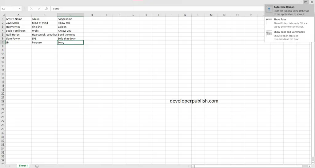
- Click on the Show Tabs option to display the Ribbon tabs without the commands.
- To access the commands in the Show Tabs option, click any of the tabs.
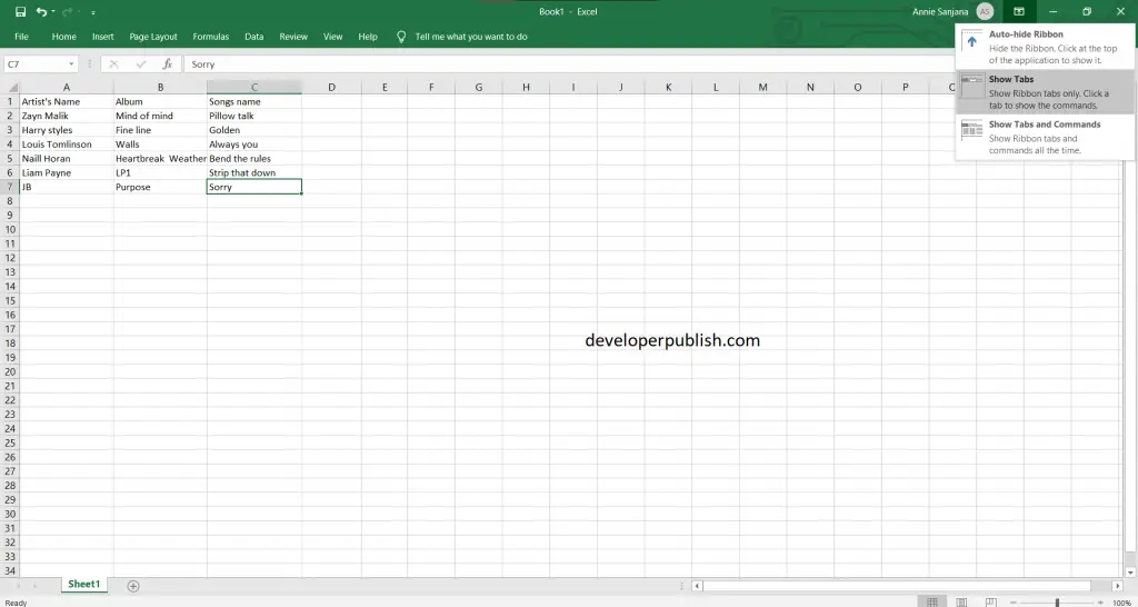
- Click on the Show Tabs and Commands to show the Ribbon with all tabs and full commands.
- This option is the default view in the excel sheet.