What is relative and absolute in excel

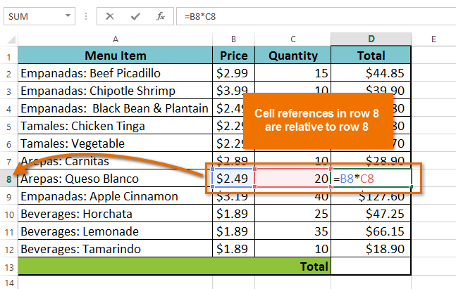
By default, a cell reference is a relative reference, which means that the reference is relative to the location of the cell. If, for example, you refer to cell A2 from cell C2, you are actually referring to a cell that is two columns to the left (C minus A)—in the same row (2). When you copy a formula that contains a relative cell reference, that reference in the formula will change.

As an example, if you copy the formula =B4*C4 from cell D4 to D5, the formula in D5 adjusts to the right by one column and becomes =B5*C5. If you want to maintain the original cell reference in this example when you copy it, you make the cell reference absolute by preceding the columns (B and C) and row (2) with a dollar sign ($). Then, when you copy the formula =$B$4*$C$4 from D4 to D5, the formula stays exactly the same.

Less often, you may want to mixed absolute and relative cell references by preceding either the column or the row value with a dollar sign—which fixes either the column or the row (for example, $B4 or C$4).

To change the type of cell reference:

1. Select the cell that contains the formula.

2. In the formula bar , select the reference that you want to change.

3. Press F4 to switch between the reference types.

   The table below summarizes how a reference type updates if a formula containing the reference is copied two cells down and two cells to the right.

For a formula being copied:	If the reference is:	It changes to:
	$A$1 (absolute column and absolute row)	$A$1 (the reference is absolute)
	A$1 (relative column and absolute row)	C$1 (the reference is mixed)
	$A1 (absolute column and relative row)	$A3 (the reference is mixed)
	A1 (relative column and relative row)	C3 (the reference is relative)

Cell reference is the address or name of a cell or a range of cells. It is the combination of column name and row number. It helps the software to identify the cell from where the data/value is to be used in the formula. We can reference the cell of other worksheets and also of other programs.

• Referencing the cell of other worksheets is known as External referencing.
• Referencing the cell of other programs is known as Remote referencing.

There are two types of cell references in Excel:  

• Relative reference
• Absolute reference

Relative Reference

Relative reference is the default cell reference in Excel. It is simply the combination of column name and row number without any dollar ($) sign. When you copy the formula from one cell to another the relative cell address changes depending on the relative position of column and row. C1, D2, E4, etc are examples of relative cell references. Relative references are used when we want to perform a similar operation on multiple cells and the formula must change according to the relative address of column and row.

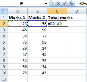
For example, We want to add the marks of two subjects entered in column A and column B and display the result in column C. Here, we will use relative reference so that the same rows of column’s A and B are added.

Steps to Use Relative Reference:

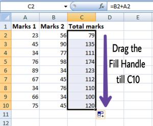
Step 1: We write the formula in any cell and press enter so that it is calculated. In this example, we write the formula(= B2 + A2) in cell C2 and press enter to calculate the formula.

Step 2: Now click on the Fill handle at the corner of cell which contains the formula(C2).

Step 3: Drag the Fill handle up to the cells you want to fill. In our example, we will drag it till cell C10.

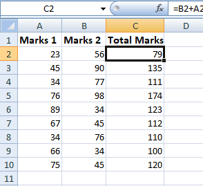
Step 4: Now we can see that the addition operation is performed between the cell A2 and B2, A3 and B3 and so on.

Step 5: You can double-click on any cell to check that the operation is performed in between which cells.

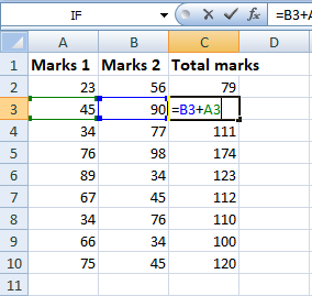
Thus, in the above example, we see that the relative address of cell A2 changes to A3, A4, and so on, similarly the relative address changes for column B, depending on the relative position of the row.

Absolute Reference

Absolute reference is the cell reference in which the row and column are made constant by adding the dollar ($) sign before the column name and row number. The absolute reference does not change as you copy the formula from one cell to other. If either the row or the column is made constant then it is known as a mixed reference. You can also press the F4 key to make any cell reference constant. $A$1, $B$3 are examples of absolute cell reference.

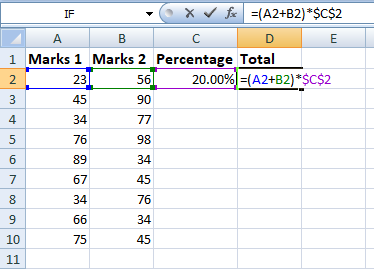
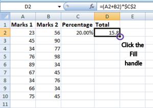
For example, We want to multiply the sum of marks of two subjects, entered in column A and column B, with the percentage entered in cell C2 and display the result in column D. Here, we will use absolute reference so that the address of cell C2 remains constant and does not change with the relative position of column and rows.

Steps to Use Absolute Reference:

Step 1: We write the formula in any cell and press enter so that it is calculated. In this example, we write the formula(=(A2+B2)*$C$2) in cell D2 and press enter to calculate the formula.

Step 2: Now click on the Fill handle at the corner of cell which contains the formula(D2).

Step 3: Drag the Fill handle up to the cells you want to fill. In our example, we will drag it till cell D10.

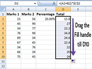
Step 4: Now we can see that the percentage is calculated in column D.

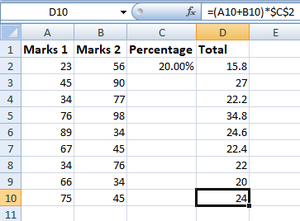
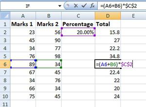
Step 5: You can double-click on any cell to check that the operation is performed in between which cells, and we see that the address of cell C2 does not change.

Thus, in the above example we see that the address of cell C2 is not changed whereas the address of column A and B changes with the relative position of the row and column, this happened because we used the absolute address of the cell C2.

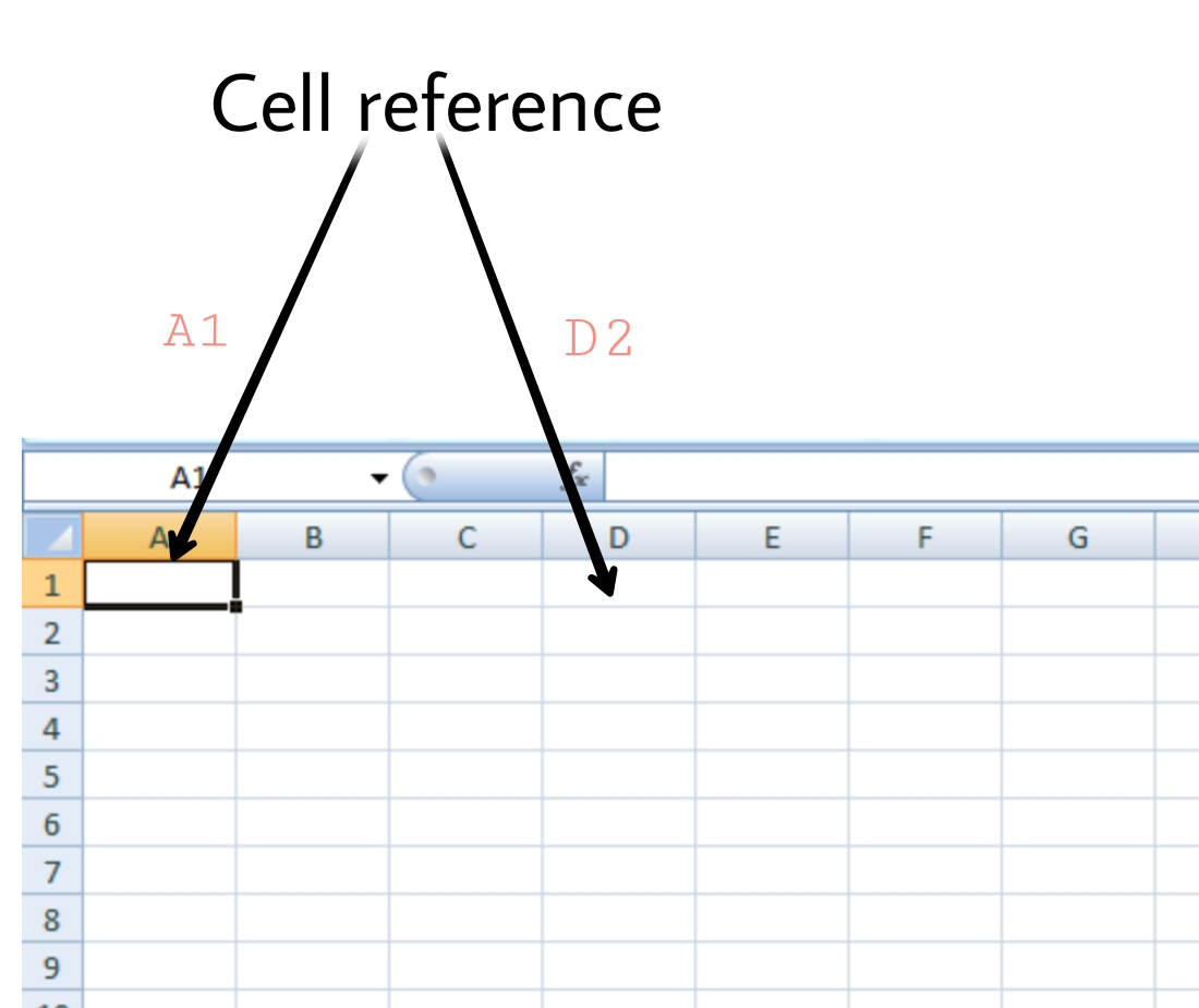
A worksheet in Excel is made up of cells. These cells can be referenced by specifying the row value and the column value.

For example, A1 would refer to the first row (specified as 1) and the first column (specified as A). Similarly, B3 would be the third row and second column.

The power of Excel lies in the fact that you can use these cell references in other cells when creating formulas.

Now there are three kinds of cell references that you can use in Excel:

• Relative Cell References
• Absolute Cell References
• Mixed Cell References

Understanding these different types of cell references will help you work with formulas and save time (especially when copy-pasting formulas).

What are Relative Cell References in Excel?

Let me take a simple example to explain the concept of relative cell references in Excel.

Suppose I have a data set shown below:

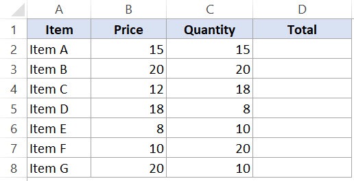
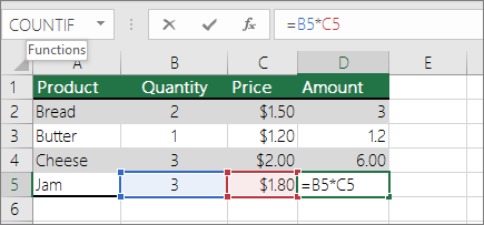
To calculate the total for each item, we need to multiply the price of each item with the quantity of that item.

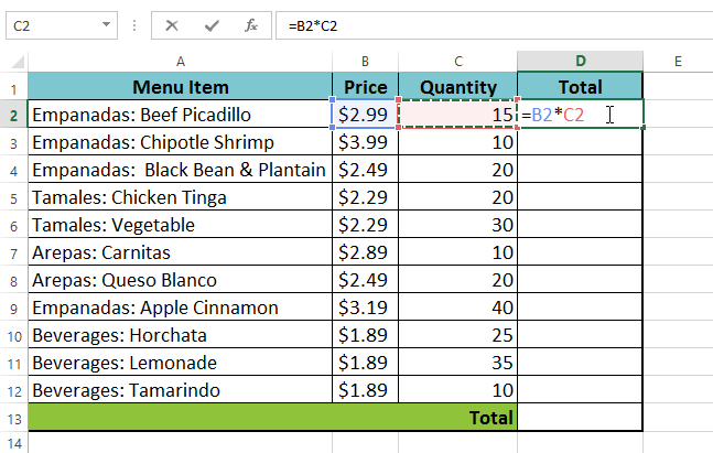
For the first item, the formula in cell D2 would be B2* C2 (as shown below):

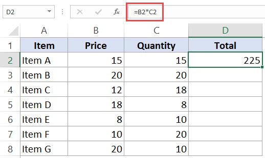
Now, instead of entering the formula for all the cells one by one, you can simply copy cell D2 and paste it into all the other cells (D3:D8). When you do it, you will notice that the cell reference automatically adjusts to refer to the corresponding row. For example, the formula in cell D3 becomes B3*C3 and the formula in D4 becomes B4*C4.

These cell references that adjust itself when the cell is copied are called relative cell references in Excel.

When to Use Relative Cell References in Excel?

Relative cell references are useful when you have to create a formula for a range of cells and the formula needs to refer to a relative cell reference.

In such cases, you can create the formula for one cell and copy-paste it into all cells.

What are Absolute Cell References in Excel?

Unlike relative cell references, absolute cell references don’t change when you copy the formula to other cells.

For example, suppose you have the data set as shown below where you have to calculate the commission for each item’s total sales.

The commission is 20% and is listed in cell G1.

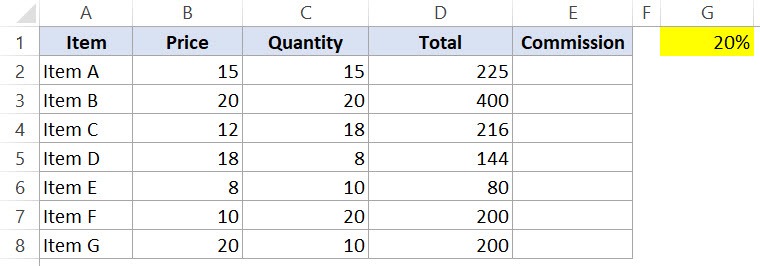
To get the commission amount for each item sale, use the following formula in cell E2 and copy for all cells:

=D2*$G$1

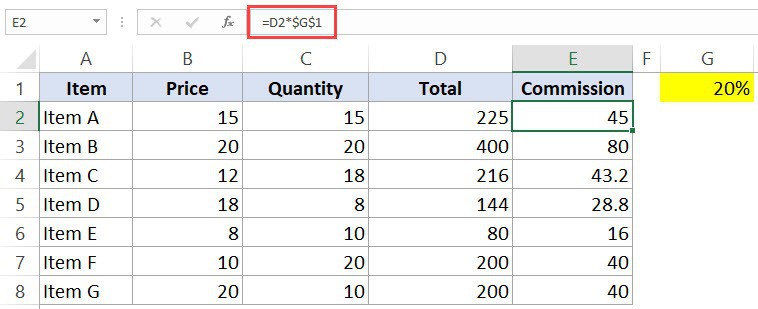
Note that there are two dollar signs ($) in the cell reference that has the commission – $G$2.

What does the Dollar ($) sign do?

A dollar symbol, when added in front of the row and column number, makes it absolute (i.e., stops the row and column number from changing when copied to other cells).

For example, in the above case, when I copy the formula from cell E2 to E3, it changes from =D2*$G$1 to =D3*$G$1.

Note that while D2 changes to D3, $G$1 doesn’t change.

Since we have added a dollar symbol in front of ‘G’ and ‘1’ in G1, it wouldn’t let the cell reference change when it’s copied.

Hence this makes the cell reference absolute.

When to Use Absolute Cell References in Excel?

Absolute cell references are useful when you don’t want the cell reference to change as you copy formulas. This could be the case when you have a fixed value that you need to use in the formula (such as tax rate, commission rate, number of months, etc.)

While you can also hard code this value in the formula (i.e., use 20% instead of $G$2), having it in a cell and then using the cell reference allows you to change it at a future date.

For example, if your commission structure changes and you’re now paying out 25% instead of 20%, you can simply change the value in cell G2, and all the formulas would automatically update.

What are Mixed Cell References in Excel?

Mixed cell references are a bit more tricky than the absolute and relative cell references.

There can be two types of mixed cell references:

• The row is locked while the column changes when the formula is copied.
• The column is locked while the row changes when the formula is copied.

Let’s see how it works using an example.

Below is a data set where you need to calculate the three tiers of commission based on the percentage value in cell E2, F2, and G2.

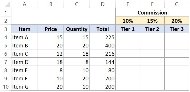
Now you can use the power of mixed reference to calculate all these commissions with just one formula.

Enter the below formula in cell E4 and copy for all cells.

=$B4*$C4*E$2

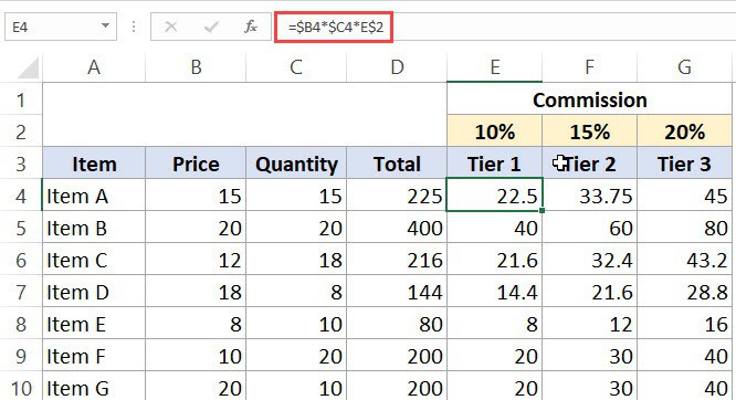
The above formula uses both kinds of mixed cell references (one where the row is locked and one where the column is locked).

Let’s analyze each cell reference and understand how it works:

• $B4 (and $C4) –  In this reference, the dollar sign is right before the Column notation but not before the Row number. This means that when you copy the formula to the cells on the right, the reference will remain the same as the column is fixed. For example, if you copy the formula from E4 to F4, this reference would not change. However, when you copy it down, the row number would change as it is not locked.
• E$2 – In this reference, the dollar sign is right before the row number, and the Column notation has no dollar sign. This means that when you copy the formula down the cells, the reference will not change as the row number is locked. However, if you copy the formula to the right, the column alphabet would change as it’s not locked.

How to Change the Reference from Relative to Absolute (or Mixed)?

To change the reference from relative to absolute, you need to add the dollar sign before the column notation and the row number.

For example, A1 is a relative cell reference, and it would become absolute when you make it $A$1.

If you only have a couple of references to change, you may find it easy to change these references manually. So you can go to the formula bar and edit the formula (or select the cell, press F2, and then change it).

However, a faster way to do this is by using the keyboard shortcut – F4.

When you select a cell reference (in the formula bar or in the cell in edit mode) and press F4, it changes the reference.

Suppose you have the reference =A1 in a cell.

Here is what happens when you select the reference and press the F4 key.

• Press F4 key once: The cell reference changes from A1 to $A$1 (becomes ‘absolute’ from ‘relative’).
• Press F4 key two times: The cell reference changes from A1 to A$1 (changes to mixed reference where the row is locked).
• Press F4 key three times: The cell reference changes from A1 to $A1 (changes to mixed reference where the column is locked).
• Press F4 key four times: The cell reference becomes A1 again.

You May Also Like the Following Excel Tutorials:

• How to Copy and Paste Formulas in Excel without Changing Cell References
• How to Lock Cells in Excel.
• Excel Freeze Panes: Use it to Lock Row/Column Headers.
• How to Lock Formulas in Excel.
• How to Reference Another Sheet or Workbook in Excel
• How to Find Circular Reference in Excel
• Using A1 or R1C1 Reference Notation in Excel (& How to Change These)

/en/excelformulas/complex-formulas/content/

Introduction

There are two types of cell references: relative and absolute. Relative and absolute references behave differently when copied and filled to other cells. Relative references change when a formula is copied to another cell. Absolute references, on the other hand, remain constant no matter where they are copied.

Optional: Download our example file for this lesson.

Watch the video below to learn more about cell references.

Relative references

By default, all cell references are relative references. When copied across multiple cells, they change based on the relative position of rows and columns. For example, if you copy the formula =A1+B1 from row 1 to row 2, the formula will become =A2+B2. Relative references are especially convenient whenever you need to repeat the same calculation across multiple rows or columns.

To create and copy a formula using relative references:

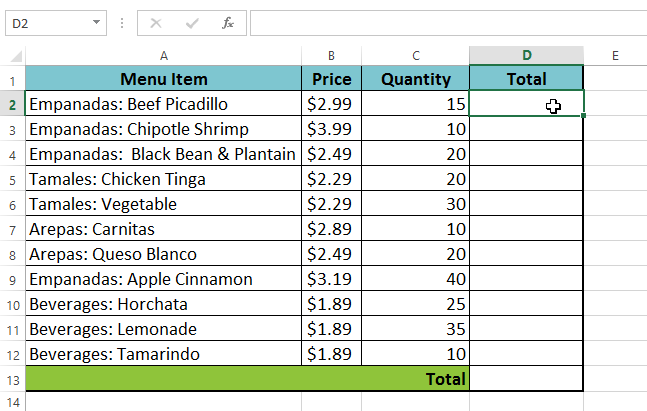
In the following example, we want to create a formula that will multiply each item’s price by the quantity. Rather than create a new formula for each row, we can create a single formula in cell D2 and then copy it to the other rows. We’ll use relative references so the formula correctly calculates the total for each item.

1. Select the cell that will contain the formula. In our example, we’ll select cell D2.

   

2. Enter the formula to calculate the desired value. In our example, we’ll type =B2*C2.

   

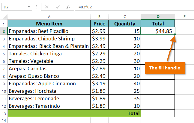
3. Press Enter on your keyboard. The formula will be calculated, and the result will be displayed in the cell.
4. Locate the fill handle in the lower-right corner of the desired cell. In our example, we’ll locate the fill handle for cell D2.

   

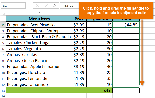
5. Click, hold, and drag the fill handle over the cells you wish to fill. In our example, we’ll select cells D3:D12.

   

6. Release the mouse. The formula will be copied to the selected cells with relative references and the values will be calculated in each cell.

   

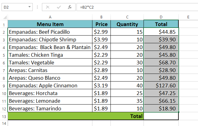
You can double-click the filled cells to check their formulas for accuracy. The relative cell references should be different for each cell, depending on its row.

Absolute references

There may be times when you do not want a cell reference to change when filling cells. Unlike relative references, absolute references do not change when copied or filled. You can use an absolute reference to keep a row and/or column constant.

An absolute reference is designated in a formula by the addition of a dollar sign ($) before the column and row. If it precedes the column or row (but not both), it’s known as a mixed reference.

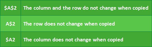
You will use the relative (A2) and absolute ($A$2) formats in most formulas. Mixed references are used less frequently.

When writing a formula in Microsoft Excel, you can press the F4 key on your keyboard to switch between relative, absolute, and mixed cell references, as shown in the video below. This is an easy way to quickly insert an absolute reference.

To create and copy a formula using absolute references:

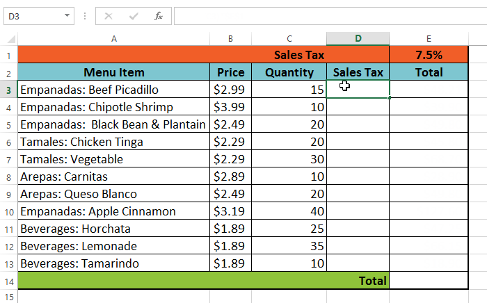
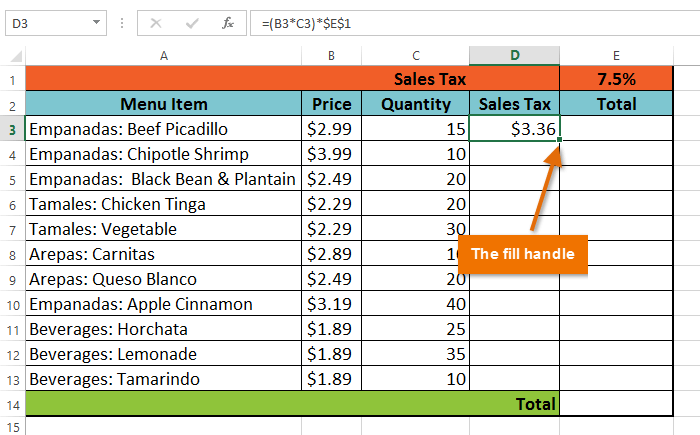
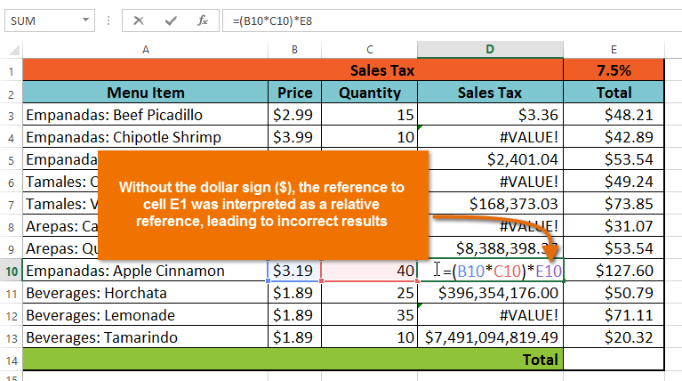
In our example, we’ll use the 7.5% sales tax rate in cell E1 to calculate the sales tax for all items in column D. We’ll need to use the absolute cell reference $E$1 in our formula. Because each formula is using the same tax rate, we want that reference to remain constant when the formula is copied and filled to other cells in column D.

1. Select the cell that will contain the formula. In our example, we’ll select cell D3.

   

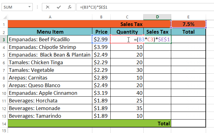
2. Enter the formula to calculate the desired value. In our example, we’ll type =(B3*C3)*$E$1.

   

3. Press Enter on your keyboard. The formula will calculate, and the result will display in the cell.
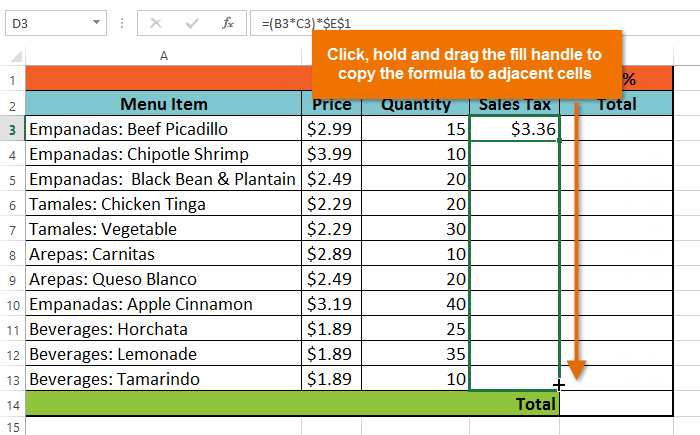
4. Locate the fill handle in the lower-right corner of the desired cell. In our example, we’ll locate the fill handle for cell D3.

   
5. Click, hold, and drag the fill handle over the cells you wish to fill, cells D4:D13 in our example.

   

6. Release the mouse. The formula will be copied to the selected cells with an absolute reference, and the values will be calculated in each cell.

   

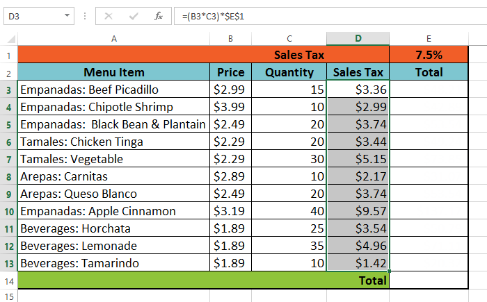
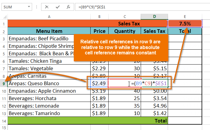
You can double-click the filled cells to check their formulas for accuracy. The absolute reference should be the same for each cell, while the other references are relative to the cell’s row.

Be sure to include the dollar sign ($) whenever you’re making an absolute reference across multiple cells. The dollar signs were omitted in the example below. This caused the spreadsheet to interpret it as a relative reference, producing an incorrect result when copied to other cells.

Using cell references with multiple worksheets

Most spreadsheet programs allow you to refer to any cell on any worksheet, which can be especially helpful if you want to reference a specific value from one worksheet to another. To do this, you’ll simply need to begin the cell reference with the worksheet name followed by an exclamation point (!). For example, if you wanted to reference cell A1 on Sheet1, its cell reference would be Sheet1!A1.

Note that if a worksheet name contains a space, you will need to include single quotation marks (‘ ‘) around the name. For example, if you wanted to reference cell A1 on a worksheet named July Budget, its cell reference would be ‘July Budget’!A1.

To reference cells across worksheets:

In our example below, we’ll refer to a cell with a calculated value between two worksheets. This will allow us to use the exact same value on two different worksheets without rewriting the formula or copying data between worksheets.

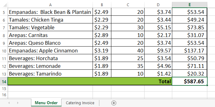
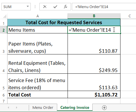
1. Locate the cell you wish to reference, and note its worksheet. In our example, we want to reference cell E14 on the Menu Order worksheet.

   
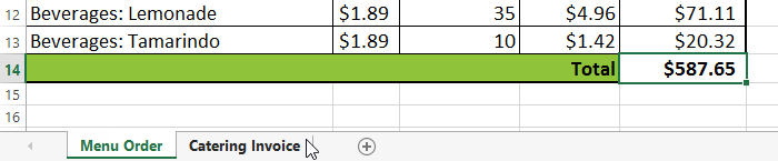
2. Navigate to the desired worksheet. In our example, we’ll select the Catering Invoice worksheet.

   

3. The selected worksheet will appear.
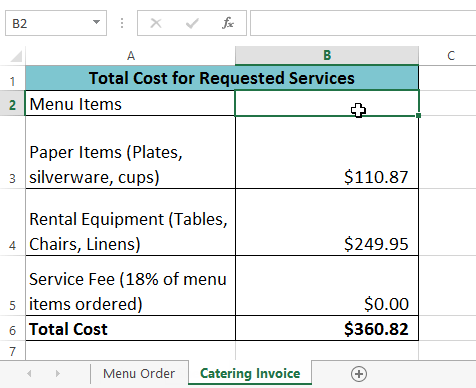
4. Locate and select the cell where you want the value to appear. In our example, we’ll select cell B2.

   

5. Type the equals sign (=), the sheet name followed by an exclamation point (!), and the cell address. In our example, we’ll type =’Menu Order’!E14.

   

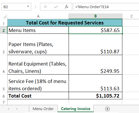
6. Press Enter on your keyboard. The value of the referenced cell will appear. If the value of cell E14 changes on the Menu Order worksheet, it will be updated automatically on the Catering Invoice worksheet.

   

If you rename your worksheet at a later point, the cell reference will be updated automatically to reflect the new worksheet name.

Challenge!

1. Open an existing Excel workbook. If you want, you can use the example file for this lesson.
2. Create a formula that uses a relative reference. If you are using the example, use the fill handle to fill in the formula in cells E4 through E14. Double-click a cell to see the copied formula and the relative cell references.
3. Create a formula that uses an absolute reference. If you are using the example, correct the formula in cell D4 to refer only to the tax rate in cell E2 as an absolute reference, then use the fill handle to fill the formula from cells D4 to D14.
4. Try referencing a cell across worksheets. If you are using the example, create a cell reference in cell B3 on the Catering Invoice worksheet for cell E15 on the Menu Order worksheet.

/en/excelformulas/functions/content/

Highlight the cell containing the formula you want to have changed to an absolute or relative reference. Click the formula box (shown below) or highlight the formula and press the F4 key to switch between an absolute and relative cell reference.

How do you convert absolute to relative?

Convert reference from absolute to relative

1. 1# select the cell that contains the reference you want to change.
2. 2# select the reference of references that you want to convert.
3. 3# press F4 key three times.
4. Note: if you type a relative reference into formula box, then press F4, the reference will change to absolute.

How do you do a relative reference in Excel?

By default, every cell in Excel has a relative reference. In relative references, type “=A1+A2” in cell A3, copy and paste the formula in cell B3, and the formula automatically changes to “=B1+B2.” In absolute references, the cell address does not change when the formula is copied.

What is absolute and relative reference in Excel?

There are two types of cell references: relative and absolute.Relative references change when a formula is copied to another cell. Absolute references, on the other hand, remain constant no matter where they are copied.

How do you dynamically reference a cell in Excel?

To create an Excel dynamic reference to any of the above named ranges, just enter its name in some cell, say G1, and refer to that cell from an Indirect formula =INDIRECT(G1) .

How do you make an absolute reference in Excel without F4?

This is easily fixed! Just hold down the Fn key before you press F4 and it’ll work.

What is absolute referencing in Excel?

An absolute reference in Excel refers to a reference that is “locked” so that rows and columns won’t change when copied. Unlike a relative reference, an absolute reference refers to an actual fixed location on a worksheet. To create an absolute reference in Excel, add a dollar sign before the row and column.

How do you change an absolute reference to a mixed reference?

Switch between relative, absolute, and mixed references

1. Select the cell that contains the formula.
2. In the formula bar. , select the reference that you want to change.
3. Press F4 to switch between the reference types.

How do you use absolute cell reference in Excel?

Select another cell, and then press the F4 key to make that cell reference absolute. You can continue to press F4 to have Excel cycle through the different reference types.

What is difference between absolute and relative?

Summary: 1. Relative is always in proportion to a whole. Absolute is the total of all existence.

What is an Xlookup in Excel?

Use the XLOOKUP function to find things in a table or range by row.With XLOOKUP, you can look in one column for a search term, and return a result from the same row in another column, regardless of which side the return column is on.

How do I create a dynamic spreadsheet?

#1 – Using Tables to create Dynamic Tables in Excel

1. Select the data, i.e., A1:E6.
2. In the Insert tab, click on Tables under the tables section.
3. A dialog box pops up.
4. Our Dynamic Range is created.
5. Select the data and in the Insert Tab under the excel tables section, click on pivot tables.

How do I create a dynamic worksheet?

Click any cell in the Excel table. On the Insert tab, in the Tables group, click the PivotTable button (not the arrow). The Create PivotTable dialog box opens. Verify that the DailyVolumes table name appears in the Table/Range field and that the New Worksheet option is selected.

What does F5 key do in Excel?

F5. Displays the Go To dialog box. For example, to select cell C15, in the Reference box, type C15, and click OK. Note: you can also select named ranges, or click Special to quickly select all cells with formulas, comments, conditional formatting, constants, data validation, etc.

What does F5 do in Excel?

Shortcut keys in Excel – Function Keys (6 of

Key	Description
F3	F3: Displays the Paste Name dialog box. Available only if names have been defined in the workbook.
	Shift+F3: Displays the Insert Function dialog box.
F5	F5: Displays the Go To dialog box.
	Ctrl+F5: Restores the window size of the selected workbook window.

How do you copy absolute values in Excel?

To copy the formula entered using absolute references and preserve the cell references, select the cell containing the formula and copy it (Ctrl + C) and click the destination cell into which you want to paste the formula.

What is F4 on Mac Excel?

The shortcut to toggle absolute and relative references is F4 in Windows, while on a Mac, its Command T. For a complete list of Windows and Mac shortcuts, see our side-by-side list. If you want to see more Excel shortcuts for the Mac in action, see our our video tips.

How do I turn off relative references in Excel?

Click File > Options in Excel. Click the Formulas option on the left side menu. In the Working with Formulas section, uncheck the box that says “Use table names in formulas”. Press OK.

What is the difference between relative change and absolute change?

Absolute change refers to the simple difference in the indicator over two periods in time, i.e. Relative change expresses the absolute change as a percentage of the value of the indicator in the earlier period, i.e.

How are absolute and relative location different?

An absolute location describes a precise point on Earth or another defined space. A relative location describes where something else by using another, familiar feature as a reference point.

Why is relative better than absolute?

Relative changes on small numbers can appear to be more significant than they are. This is because a small absolute change in the number can result in a large percentage change. So if I got a $50 return on my $10 investment, my relative change was a 400% increase.

Excel Relative References

---

Relative and Absolute References

Cells in Excel have unique references, which is its location.

References are used in formulas to do calculations, and the fill function can be used to continue formulas sidewards, downwards and upwards.

Excel has two types of references:

1. Relative references
2. Absolute references

Absolute reference is a choice we make. It is a command which tells Excel to lock a reference.

The dollar sign ($) is used to make references absolute.

Example of relative reference: A1

Example of absolute reference: $A$1

---

Relative reference

References are relative by default, and are without dollar sign ($).

The relative reference makes the cells reference free. It gives the fill function freedom to continue the order without restrictions.

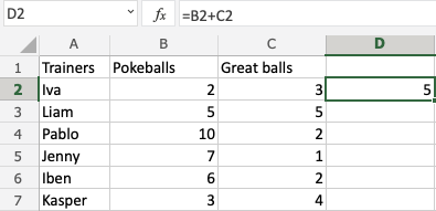
Let’s have a look at a relative reference example, helping the Pokemon trainers to count their Pokeballs (B2:B7) and Great balls (C2:C7).

The result is: D2(5):

Next, fill the range D2:D7:

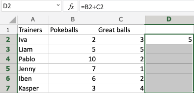
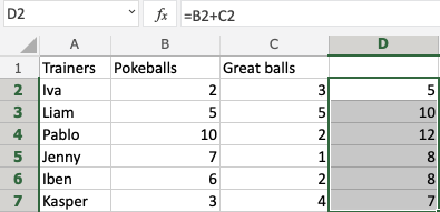
The references being relative allows the fill function to continue the formula for rows downwards.

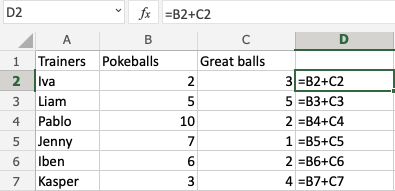
Have a look at the formulas in D2:D7. Notice that it calculates the next row as you fill.

---

---

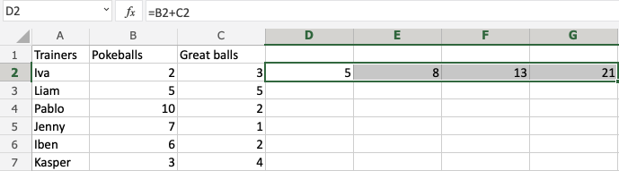
A Non-Working Example

Let’s try an example that will not work.

Fill D2:G2, filling to the right instead of downwards. Resulting in strange numbers:

Have a look at the formulas.

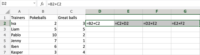
It assumes that we are calculating sidewards and not downwards.

The numbers that we want to calculate need to be in the same direction as we fill.

---

---

While working or learning Excel, you’ve must hear of Relative and Absolute referencing of cells and ranges. Absolute referencing is also called locking of cells. Understanding of Relative and Absolute Reference in Excel is very important to work effectively on Excel. So let’s get started.

Absolute Referencing or Locking Cell in Formula

When you don’t want to change the referenced cell while you copy a formula cell somewhere else, you use Absolute Referencing using $ sign. Let’s see an example.

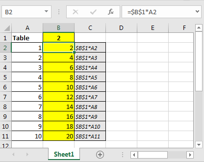
Create A Table Generator

In this example, you need to create a table generator. You will write a number in Cell B1. The Range B2: B11 should display the table of that number.

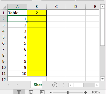
You just need to multiply B1 to A1 and then just copy the formula below. It won’t work my friend but let’s just try this…

In cell B2, write this formula and copy it in below cell.

=B1*A2

What happened? ???? This is not the table of 2 you learned in primary school. Ok lets see whats going on here.

When copy or drag down the formula cell, the reference to B1 also changes. See below image.

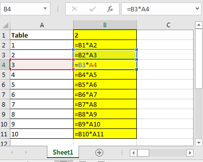
This is called Relative Referencing. So how do we lock cell B2 or say give an Absolute Reference of a cell?

• Just put a $ sign before column character and row number to lock the cell in excel. Eg. ($A$1).
• Or select the range in formula and hit F4 button.

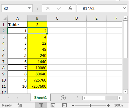
The formula in cell B2 will look like this.

=$B$1*A2

Copy it to the below cells or anywhere else. The reference to B1 will not change.

Relative Referencing or Locking Cell in Formula

In the above example, the reference to cell A2 is relative. The relative cell changes relatively when the formula is copied to another cell. As happens to A2 in the above example. Where the cell B2 is copied to B3 the reference of A2 changes to A3.

You can make row absolute and column relative or vice versa by just putting $ sign before a column or row number.

For example eg; $A1 means the only column a is locked but the row is not. If you copy this cell to left the column A will not change but when to copy the formula down the row number will change.

Related Articles:

How to use Dynamic Worksheet Reference in Excel

How to use Relative and Absolute Reference in Excel in Excel

How to use Shortcut To Toggle Between Absolute and Relative References in Excel

How to Count Unique Values In Excel

All About Excel Named Ranges in Excel

Popular Articles:

50 Excel Shortcuts to Increase Your Productivity

How to use the VLOOKUP Function in Excel

How to use the COUNTIF function in Excel

How to use the SUMIF Function in Excel

As already discussed in the article “How to Create a Formula in Excel“. If a cell contains a formula copied to another cell, it will generate a cell containing a formula as well. By default, the cell address used by the formula will change to adjust the location of the new cell.

Excel provides three options to set a reference to the cell if the cell contains a formula copied, i.e., relative cell reference, absolute cell reference and mixed cell reference

Relative Cell Reference

What is Relative Cell Reference?

When a cell address contains a formula copied and cell address changing according to the new cell address location, that is a relative cell reference. Relative Reference excels default behavior for all formulas.

How to Use Relative Reference in Excel

There is no specific way how to use relative reference in excel because the relative cell reference is the default cell reference used in excel. Each cell address used in creating formulas by default uses a relative cell reference.

Relative Cell Reference Example

For example, there are data such as the image below. Mr. Fulan is a very kind person :). He bought two iPhoneXs for both his parents, 1 Galaxy S9 + for his wife, 3 Moto G6 for his sisters and 4 Honor 7X for his friends. How much money should be paid to buy all these gifts?

To find out how much money spent by Mr. Fulan. First, calculate the subtotal for each cell phone by multiplying the price and the quantity of each cell phone.

Here are the steps for calculating subtotals.

1. Place the cursor in cell E2
2. Type the equal sign “=”
3. Point the cursor to cell C2
4. Type the asterisk sign “*”
5. Point the cursor to cell D2
6. Press the ENTER key

The result is the price to be paid for two iPhoneX 256GB. What about the other items subtotal? Should the formula be typed one by one for each cell phone? Of course not. If there are many items, then it will be a very time-wasting.

The solution is simple, do a copy (CTRL+C) in cell E2 that already contains a formula, then paste (CTRL+V) in the range E3:E5. The results are as shown below.

The subtotal of each item differs from the subtotal of the first item, why this happens? We did copy the existing data in cell E2, why data in range E3:E5 is not the same as the data in cell E2?

If a cell containing a formula copied, the formula is copied, not the value. Excel will copy the formula =C2*D2 in cell E2. If placed 1 row below, then the formula will change to =C3*D3 (shifted down 1 row), if moved two rows below the formula change to =C4*D4 (moved down two rows) and so on.

That’s called a relative cell reference. Thanks to Excel who has made the relative cell reference. With this, there is no need to create a formula one by one for each item.

Absolute Cell Reference

What is an Absolute Cell Reference?

The absolute cell reference is the opposite of relative cell reference. If the formula using a relative cell reference is copied and placed in a new location, then the cell address will change relatively according to the new position.

The cell address of formula with absolute reference will not change when copied and put in a new location.

How to Make an Absolute Reference in Excel

The absolute cell reference sign is a $ in front of the column letter and row number. To use an absolute cell reference, you can type the $ sign directly or by pressing the F4 key once.

Absolute Cell Reference Example

For example, there are data such as the image below. The data is like the previous case with the addition of discount data. How much the discount for each item?

The formula to calculate the discounts is the multiplication between subtotal1 data in column E with the existing discount data in cell C2.

1. Place the cursor in cell F5
2. Type the equal sign “=”
3. Point the cursor to cell E5
4. Type the asterisk “*”
5. Point the cursor to cell C2
6. Press the ENTER key

The result is as shown below

How about discounts on other items? Just do a copy (CTRL+C) in cell F5 then paste (CTRL+V) in the range F8:F6. The result is as shown below.

Why the results are not as expected?

Check the formula in cell F5. The subtotal1 data point to cell E5, correct and discount data point to cell C2, correct.

Check the formula in cell F6. The subtotal1 data point to cell E6, correct and discount data point to cell C3, wrong.

Check the formula in cell F7. The subtotal1 data point to cell E7, correct and discount data point to cell C4, wrong.

Check the formula in cell F8. The subtotal1 data point to cell E8, correct and discount data point to cell C5, wrong.

The wrong formula is a formula in the discount data section, when the formula is copied down the cell address point to discount data shifted down too. It should remain pointing to cell C2.

The solution is to use the absolute cell reference, when the formula copied and placed in a new place, cell address remains unchanged and point to the same address.

1. Place the cursor in cell F5
2. Do an edit by pressing the F2 key
3. Block cell address C2
4. Press the F4 key once; the cell address C2 turns to $C$2; there is a dollar sign in front of column letter and row number. It’s mean cell address C2 uses an absolute cell reference
5. Press the ENTER key
6. Do a copy in cell F5 (CTRL+C) then paste (CTRL+V) in the range F6:F8

The result is as shown below, cell address C2 does not change even if copied down.

Absolute vs. Relative Cell Reference

What is the difference between absolute cell reference and relative cell reference? As already explained above, the cell address with a relative cell reference will change when copied and placed to a new place, while the cell address with an absolute cell reference remains unchanged when copied and put to a new location. Which one will be used depending on condition.

Mixed Cell Reference

What is a Mixed Cell Reference?

The mixed cell reference is a combination of the relative and absolute cell reference. When using a relative cell reference, then everything either column or row is relative as well when using absolute cell reference everything becomes absolute.

Mixed cell reference can combine both. Relative in the column and absolute in a row or otherwise absolute in column and relative in a row.

How to Create a Mixed Reference in Excel

To use a mixed cell reference could use a dollar sign “$” in front of the column letters or row numbers. The placement of the dollar sign specifies which column/row will be absolute.

The cell address $A1 shows column A using absolute cell reference while row 1 uses relative cell reference. Pressing F4 key three times will generate this mixed cell reference.

The cell address A$1 shows the opposite, column using relative cell reference and row uses absolute cell reference. Pressing F4 key twice will generate this mixed cell reference.

Mixed Cell Reference Example

Suppose there is data like the picture below. It’s like the previous example with the addition of sales tax data. How much is the sales tax for each item? Is it possible to calculate sales tax just by copying the formula to calculate discounts?

1. Select range F5:F8 then do a copy (CTRL+C)
2. Place the cursor in cell G5
3. Do a paste (CTRL+V)

The results are as shown below.

The resulting number is not as desired, why can it be like this?

Check the formula in cell G5. Subtotal1 cell reference should remain pointing to cell E5 but shifted right 1 column point to cell F5. While sales tax cell reference which should move right 1 column point to cell D2, remains point to cell C2.

For subtotal1 cell reference, when copied to the right, from column F (Discount) to column G (Sales Tax) column position unchanged, remain in column D. Conversely, if copied down from row 5 to row 8, row position must change to adjust to the new location.

So, the cell reference for subtotal1 is written $E5, column uses absolute reference, indicated by the $ sign and row using relative reference.

For discount cell reference, when copied to the right, the position of the column should change. Conversely, if copied down the row position remain unchanged.

So, the cell reference for the discount is written C$2, column using a relative reference and row uses the absolute reference, indicated by the $ sign.

Edit the formula in cell F5. Block cell E5 then press F4 key three times; block cell C2 then press the F4 once. The formula becomes =$E5*C$2, then press the ENTER key.

To calculate the discount on other items. Do a copy (CTRL+C) in cell F5, and then do a paste (CTRL+V) in the range F6:F8. To calculate sales tax, do a paste again (CTRL+V) in range G5:G8.

The results are as shown below.

Check the formula in cell F5. Subtotal1 cell reference point to cell E5 and discount cell reference point to cell C2.

Check the formula in cell G5. Subtotal1 cell reference remains to point cell E5 and sales tax cell reference shifted right 1 column point to cell C3.

By understanding the differences of relative reference, absolute reference, and mixed reference, formula writing can be done only once for various purposes. For the above case, one formula can be used to calculate discount and sales tax at once.

3D Cell Reference

What is a 3D Reference in Excel?

3D reference is a cell reference used in multiple worksheets in a workbook that has the same data structure.

How to Do a 3D Reference in Excel

For example, there are data such as the image below; there are three worksheets. Each worksheet has the same data structure. Three columns with eight cellphone and sales data. Two sheets contain sales data for an area, and one sheet has the total sales for all regions. How does the formula to calculate the total sales of all areas?

Solution Using Addition formula

The following steps to create the formula by using the “+” sign.

1. Place cursor in cell C2, worksheet “Total”
2. Type equal sign “=”
3. Click worksheet “West”, then click cell C2
4. Type plus sign “+”
5. Click worksheet “East”, then click cell C2
6. Press the ENTER key

Below is the result of the formula

=West!C2+East!C2

To calculate total sales of another cell phone. Do a copy (CTRL+C) in cell C2, then paste (CTRL+V) in range C3:C9. The result as shown below.

This way is easy because workbook only has a few worksheets. If there are a lot of worksheets, then it will be time-consuming and increase the possibilities of error. Also, if there is a new worksheet (new area), the formula should be edited to include the sales of the new area.

The above problems can be solved using 3D reference. The SUM function will be used to calculate the total sales.

Solution Using 3D Reference

Here are the steps to create a formula using 3D reference.

1. Place the cursor in cell C2, worksheet “Total”
2. Type =SUM(
3. Click the “West” worksheet
4. Press the SHIFT key and hold
5. Click on the “East” worksheet, then release the SHIFT key
6. Click cell C2
7. Type ) “close brackets”
8. Press the ENTER button

Below is the result of the formula

=SUM(West:East!C2)

To calculate total sales of another cell phone. Do a copy (CTRL+C) in cell C2, then paste (CTRL+V) in range B3:B7. The result is as shown below.

There is no difference in results compared to the previous way. The difference shows when a new worksheet is added.

The addition of a new worksheet will automatically change the total sales without changing the formula. As a note, the new worksheet should be placed between the “West” and “East” worksheets.

External Cell Reference

What is External Cell Reference?

The external cell reference is the cell reference for the data point to another excel file (workbook).

How to Do an External Cell Reference

Suppose there are two sales areas (west, east), each of them is stored in an Excel file, and then there is another Excel file that contains the total sales from all regions.

“Please download the exercise file here”

Here are the steps to create an external reference.

1. Open all files (west.xlsx, east.xlsx and total.xlsx)
2. Select workbook total.xlsx, place the cursor in cell C2
3. Type =
4. Switch windows (CTRL+F6), select west.xlsx, click cell C2
5. Type +
6. Switch windows (CTRL+F6), select east.xlsx, click cell C2
7. Press the ENTER key

The result of the formula in cell C2 is

=[west.xlsx]West!$C$2+ [east.xlsx]East!$C$2

There is a $ sign in front of the cell address for each workbook. It’s meant the formula above using absolute reference, to change to a relative reference, remove the $ sign of each cell address.

To calculate the total sales of another cell phone. Do a copy (CTRL+C) in cell C2, then paste in range C3:C9. The results are as shown below.

If the sales data for one area is updated, then the total sales data in the workbook total.xlsx will be updated immediately.

Excel Cell Reference Practice File