
Содержание
- Свойство Worksheet.Range (Excel)
- Синтаксис
- Параметры
- Замечания
- Примеры
- Поддержка и обратная связь
- Объект Range (Excel)
- Примечания
- Пример
- Методы
- Свойства
- См. также
- Поддержка и обратная связь
- Range
- Cell, Row, Column
- Range Examples
- Fill a Range
- Move a Range
- Copy/Paste a Range
- Insert Row, Column
Свойство Worksheet.Range (Excel)
Возвращает объект Range , представляющий ячейку или диапазон ячеек.
Синтаксис
expression. Диапазон (ячейка1, ячейка2)
Выражение Переменная, представляющая объект Worksheet .
Параметры
| Имя | Обязательный или необязательный | Тип данных | Описание |
|---|---|---|---|
| Cell1 | Обязательный | Variant | Строка, которая является ссылкой на диапазон при использовании одного аргумента. Строка, которая является ссылкой на диапазон, или объект Range, если используются два аргумента. |
| Cell2 | Необязательный | Variant | Строка, которая является ссылкой на диапазон, или объект Range. Cell2 определяет другую крайность диапазона, возвращаемого свойством . |
Замечания
Cell1 и Cell2 могут быть ссылками в стиле A1 на языке макроса. Ссылки на диапазоны могут включать оператор диапазона (двоеточие), оператор пересечения (пробел) или оператор union (запятая). Они также могут включать знаки доллара, которые игнорируются. Локальное имя может быть ссылкой на диапазон. При использовании имени предполагается, что оно записано на языке макроса.
Cell1 и Cell2 могут быть объектами Range , содержащими одну ячейку, столбец, строку или любой другой диапазон ячеек.
Часто ячейки Cell1 и Cell2 являются отдельными ячейками в левом верхнем и нижнем правом углах возвращаемого диапазона.
При использовании без квалификатора объекта это свойство является ярлыком для ActiveSheet.Range (оно возвращает диапазон из активного листа; если активный лист не является листом, свойство завершается ошибкой).
При применении к объекту Range это свойство выполняется относительно объекта Range. Например, если выделено ячейка C3, возвращает ячейку D3, Selection.Range(«B1») так как она относительно объекта Range , возвращаемого свойством Selection . С другой стороны, код ActiveSheet.Range(«B1») всегда возвращает ячейку B1.
Примеры
В этом примере ячейке A1 на Листе1 присваивается значение 3,14159.
В этом примере создается формула в ячейке A1 на Листе1.
В этом примере выполняется цикл по ячейкам A1:D10 на листе 1 активной книги. Если в одной из ячеек есть значение меньше 0,001, в коде выполняется замена этого значения на 0 (ноль).
В этом примере выполняется цикл в диапазоне с именем TestRange и отображается количество пустых ячеек в диапазоне.
В этом примере стиль шрифта в ячейках A1:C5 на листе 1 активной книги задается курсивом. В примере используется синтаксис 2 свойства Range.
В этом примере сравнивается свойство Worksheet.Range , метод Application.Union и метод Application.Intersect .
Поддержка и обратная связь
Есть вопросы или отзывы, касающиеся Office VBA или этой статьи? Руководство по другим способам получения поддержки и отправки отзывов см. в статье Поддержка Office VBA и обратная связь.
Источник
Объект Range (Excel)
Представляет ячейку, строку, столбец или группу ячеек, содержащую один или несколько смежных блоков ячеек или объемный диапазон.
Хотите создавать решения, которые расширяют возможности Office на разнообразных платформах? Ознакомьтесь с новой моделью надстроек Office. Надстройки Office занимают меньше места по сравнению с надстройками и решениями VSTO, и вы можете создавать их, используя практически любую технологию веб-программирования, например HTML5, JavaScript, CSS3 и XML.
Примечания
Элемент по умолчанию объекта Range направляет вызовы без параметров в свойство Value, а вызовы с параметрами — в элемент Item. Таким образом, someRange = someOtherRange соответствует someRange.Value = someOtherRange.Value , someRange(1) соответствует someRange.Item(1) и someRange(1,1) соответствует someRange.Item(1,1) .
В разделе Пример описаны следующие свойства и методы для возврата объекта Range:
- Свойства Range и Cells объекта Worksheet
- Свойства Range и Cells объекта Range
- Свойства Rows и Columns объекта Worksheet
- Свойства Rows и Columns объекта Range
- Свойство Offset объекта Range
- Метод Union объекта Application
Пример
Чтобы вернуть объект Range, представляющий одну ячейку или диапазон ячеек, используйте синтаксис Range ( arg ), где arg обозначает диапазон. В следующем примере значение ячейки A1 помещается в ячейку A5.
В следующем примере диапазон A1:H8 заполняется случайными числами путем задания формулы для каждой ячейки в диапазоне. При использовании без квалификатора объекта (объекта слева от точки) свойство Range возвращает диапазон на активном листе. Если активное окно не является листом, метод завершается с ошибкой.
Используйте метод Activate объекта Worksheet, чтобы активировать лист перед использованием свойства Range без явного квалификатора объекта.
В следующем примере очищается содержимое диапазона Criteria.
Если используется текстовый аргумент для адреса диапазона, необходимо указать адрес в нотации стиля A1 (нельзя использовать нотацию в стиле R1C1).
Чтобы получить диапазон, содержащий все отдельные ячейки листа, используйте свойство Cells на листе. Вы можете обращаться к отдельным ячейкам, используя синтаксис Item(строка, столбец), где строка — индекс строки, а столбец — индекс столбца. Свойство Item можно пропустить, так как вызов направляется к нему с помощью элемента по умолчанию объекта Range. В следующем примере на первом листе активной книги ячейке A1 присваивается значение 24, а в ячейке B1 — значение 42.
В следующем примере задается формула для ячейки A2.
Хотя также можно использовать Range(«A1») , чтобы вернуть значение ячейки A1, иногда свойство Cells может быть удобнее, так как позволяет использовать переменную для строки или столбца. В следующем примере создаются заголовки столбцов и строк на листе Sheet1. Обратите внимание, что после активации листа можно использовать свойство Cells без явного объявления листа (оно возвращает ячейку на активном листе).
Хотя для изменения ссылок в стиле A1 можно использовать строковые функции Visual Basic, проще (и лучше при программировании) использовать нотацию Cells(1, 1) .
Используйте синтаксис_выражение_.Cells, где выражение возвращает объект Range, чтобы получить диапазон с тем же адресом, состоящий из отдельных ячеек. В таком диапазоне отдельные ячейки доступны с помощью синтаксиса Item(строка, столбец) относительно левого верхнего угла первой области диапазона. Свойство Item можно пропустить, так как вызов направляется к нему с помощью элемента по умолчанию объекта Range. В следующем примере на первом листе активной книги в ячейках C5 и D5 указывается формула.
Чтобы вернуть объект Range, используйте синтаксис Range ( ячейка1, ячейка2 ), где ячейка1 и ячейка2 — это объекты Range, указывающие начальную и конечную ячейки. В следующем примере устанавливается тип линии границы для ячеек A1:J10.
Имейте в виду, что точка перед каждым появлением свойства Cells является обязательной, если результат предыдущего оператора With нужно применять к свойству Cells. В данном случае указано, что ячейки расположены на листе один (без точки свойство Cells будет возвращать ячейки активного листа).
Чтобы получить диапазон, содержащий все строки листа, используйте свойство Rows на листе. Вы можете обращаться к отдельным строкам с помощью синтаксиса Item(строка), где строка — это индекс строки. Свойство Item можно пропустить, так как вызов направляется к нему с помощью элемента по умолчанию объекта Range.
Недопустимо указывать второй параметр свойства Item для диапазонов, состоящих из строк. Сначала нужно преобразовать их в отдельные ячейки, используя свойство Cells.
В следующем примере удаляются строки 5 и 10 первого листа активной книги.
Чтобы получить диапазон, содержащий все столбцы листа, используйте свойство Columns на листе. Вы можете обращаться к отдельным столбцам с помощью синтаксиса Item(строка) [sic], где строка — это индекс столбца в виде числа или адреса столбца в формате А1. Свойство Item можно пропустить, так как вызов направляется к нему с помощью элемента по умолчанию объекта Range.
Недопустимо указывать второй параметр свойства Item для диапазонов, состоящих из столбцов. Сначала нужно преобразовать их в отдельные ячейки, используя свойство Cells.
В следующем примере удаляются столбцы B, C, E и J первого листа активной книги.
Используйте синтаксис_выражение_.Rows, где выражение возвращает объект Range, чтобы получить диапазон, состоящий из строк первой области диапазона. Вы можете обращаться к отдельным строкам с помощью синтаксиса Item(строка), где строка — это относительный индекс строки от верхнего края первой области диапазона. Свойство Item можно пропустить, так как вызов направляется к нему с помощью элемента по умолчанию объекта Range.
Недопустимо указывать второй параметр свойства Item для диапазонов, состоящих из строк. Сначала нужно преобразовать их в отдельные ячейки, используя свойство Cells.
В следующем примере удаляются диапазоны C8:D8 и C6:D6 первого листа активной книги.
Используйте синтаксис_выражение_.Columns, где выражение возвращает объект Range, чтобы получить диапазон, состоящий из столбцов первой области диапазона. Вы можете обращаться к отдельным столбцам с помощью синтаксиса Item(строка) [sic], где строка — это относительный индекс столбца от левого края первой области диапазона, указанный в виде числа или адреса столбца в формате A1. Свойство Item можно пропустить, так как вызов направляется к нему с помощью элемента по умолчанию объекта Range.
Недопустимо указывать второй параметр свойства Item для диапазонов, состоящих из столбцов. Сначала нужно преобразовать их в отдельные ячейки, используя свойство Cells.
В следующем примере удаляются диапазоны L2:L10, G2:G10, F2:F10 и D2:D10 первого листа активной книги.
Чтобы вернуть диапазон с указанным смещением относительно другого диапазона, используйте синтаксис Offset ( строка, столбец ), где строка и столбец — это смещения строк и столбцов. В следующем примере выделяются ячейки, расположенные на три строки вниз и на один столбец вправо от ячейки в левом верхнем углу текущего выделенного фрагмента. Нельзя выбрать ячейку, которая находится не на активном листе, поэтому сначала необходимо активировать лист.
Используйте синтаксис Union ( диапазон1, диапазон2, . ) для возврата диапазонов из нескольких областей, то есть диапазонов, состоящих из двух или более смежных блоков ячеек. В следующем примере создается объект, определенный как объединение диапазонов A1:B2 и C3:D4, а затем выбирается определенный диапазон.
При работе с выделенными фрагментами, содержащими несколько областей, удобно применять свойство Areas. Оно разделяет выделенный фрагмент с несколькими областями на отдельные объекты Range, а затем возвращает объекты в виде коллекции. Используйте свойство Count в возвращенной коллекции, чтобы убедиться, что выделение содержит более одной области, как показано в следующем примере.
В этом примере используется метод AdvancedFilter объекта Range для создания списка уникальных значений, а также количества появлений этих уникальных значений в диапазоне столбца A.
Методы
Свойства
См. также
Поддержка и обратная связь
Есть вопросы или отзывы, касающиеся Office VBA или этой статьи? Руководство по другим способам получения поддержки и отправки отзывов см. в статье Поддержка Office VBA и обратная связь.
Источник
Range
A range in Excel is a collection of two or more cells. This chapter gives an overview of some very important range operations.
Cell, Row, Column
Let’s start by selecting a cell, row and column.
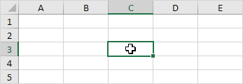
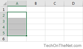
1. To select cell C3, click on the box at the intersection of column C and row 3.
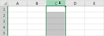
2. To select column C, click on the column C header.
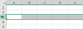
3. To select row 3, click on the row 3 header.
Range Examples
A range is a collection of two or more cells.
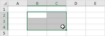
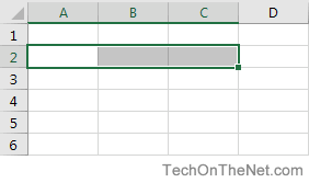
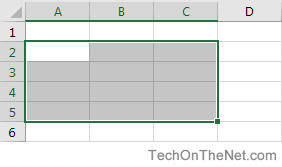
1. To select the range B2:C4, click on cell B2 and drag it to cell C4.
2. To select a range of individual cells, hold down CTRL and click on each cell that you want to include in the range.
Fill a Range
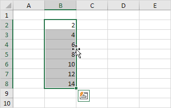
To fill a range, execute the following steps.
1a. Enter the value 2 into cell B2.
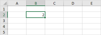
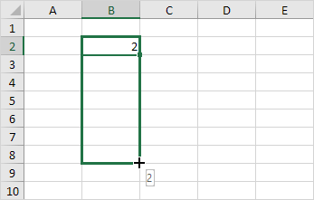
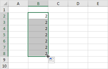
1b. Select cell B2, click on the lower right corner of cell B2 and drag it down to cell B8.
This dragging technique is very important and you will use it very often in Excel. Here’s another example.
2a. Enter the value 2 into cell B2 and the value 4 into cell B3.
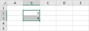
2b. Select cell B2 and cell B3, click on the lower right corner of this range and drag it down.
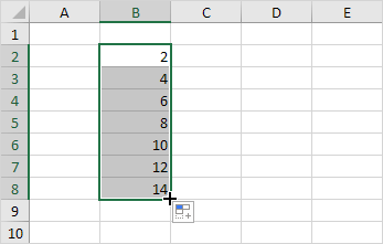
Excel automatically fills the range based on the pattern of the first two values. That’s pretty cool huh!? Here’s another example.
3a. Enter the date 6/13/2016 into cell B2 and the date 6/16/2016 into cell B3.
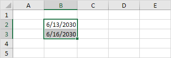
3b. Select cell B2 and cell B3, click on the lower right corner of this range and drag it down.
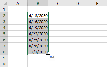
Note: visit our page about AutoFill for many more examples.
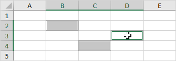
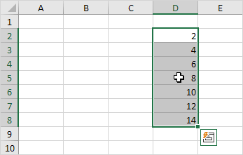
Move a Range
To move a range, execute the following steps.
1. Select a range and click on the border of the range.
2. Drag the range to its new location.
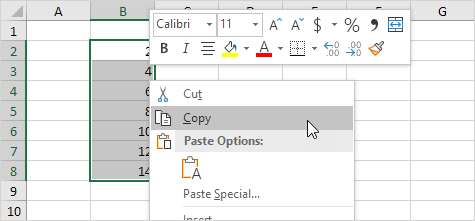
Copy/Paste a Range
To copy and paste a range, execute the following steps.
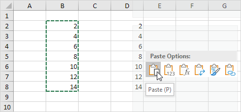
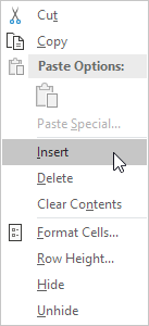
1. Select the range, right click, and then click Copy (or press CTRL + c).
2. Select the cell where you want the first cell of the range to appear, right click, and then click Paste under ‘Paste Options:’ (or press CTRL + v).
Insert Row, Column
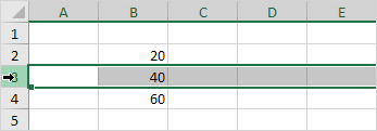
To insert a row between the values 20 and 40 below, execute the following steps.
2. Right click, and then click Insert.
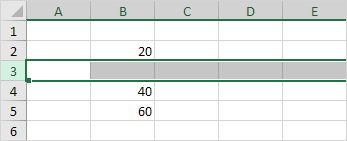
The rows below the new row are shifted down. In a similar way, you can insert a column.
Источник
A range is a group or block of cells in a worksheet that are selected or highlighted. Also, a range can be a group or block of cell references that are entered as an argument for a function, used to create a graph, or used to bookmark data.
The information in this article applies to Excel versions 2019, 2016, 2013, 2010, Excel Online, and Excel for Mac.
Contiguous and Non-Contiguous Ranges
A contiguous range of cells is a group of highlighted cells that are adjacent to each other, such as the range C1 to C5 shown in the image above.
A non-contiguous range consists of two or more separate blocks of cells. These blocks can be separated by rows or columns as shown by the ranges A1 to A5 and C1 to C5.
Both contiguous and non-contiguous ranges can include hundreds or even thousands of cells and span worksheets and workbooks.
Range Names
Ranges are so important in Excel and Google Spreadsheets that names can be given to specific ranges to make them easier to work with and reuse when referencing them in charts and formulas.
Select a Range in a Worksheet
When cells have been selected, they are surrounded by an outline or border. By default, this outline or border surrounds only one cell in a worksheet at a time, which is known as the active cell. Changes to a worksheet, such as data editing or formatting, affect the active cell.
When a range of more than one cell is selected, changes to the worksheet, with certain exceptions such as data entry and editing, affect all cells in the selected range.
There a number of ways to select a range in a worksheet. These include using the mouse, the keyboard, the name box, or a combination of the three.
To create a range consisting of adjacent cells, drag with the mouse or use a combination of the Shift and four arrow keys on the keyboard. To create ranges consisting of non-adjacent cells, use the mouse and keyboard or just the keyboard.
Select a Range for Use in a Formula or Chart
When entering a range of cell references as an argument for a function or when creating a chart, in addition to typing in the range manually, the range can also be selected using pointing.
Ranges are identified by the cell references or addresses of the cells in the upper left and lower right corners of the range. These two references are separated by a colon. The colon tells Excel to include all the cells between these start and endpoints.
Range vs. Array
At times the terms range and array seem to be used interchangeably for Excel and Google Sheets since both terms are related to the use of multiple cells in a workbook or file.
To be precise, the difference is because a range refers to the selection or identification of multiple cells (such as A1:A5) and an array refers to the values located in those cells (such as {1;2;5;4;3}).
Some functions, such as SUMPRODUCT and INDEX, take arrays as arguments. Other functions, such as SUMIF and COUNTIF, accept only ranges for arguments.
That’s not to say that a range of cell references cannot be entered as arguments for SUMPRODUCT and INDEX. These functions extract the values from the range and translate them into an array.
For example, the following formulas both return a result of 69 as shown in cells E1 and E2 in the image.
=SUMPRODUCT(A1:A5,C1:C5)
=SUMPRODUCT({1;2;5;4;3},{1;4;8;2;4})
On the other hand, SUMIF and COUNTIF do not accept arrays as arguments. So, while the formula below returns an answer of 3 (see cell E3 in the image), the same formula with an array would not be accepted.
COUNTIF(A1:A5,"<4")
As a result, the program displays a message box listing possible problems and corrections.
Thanks for letting us know!
Get the Latest Tech News Delivered Every Day
Subscribe
Find Range in Excel (Table of Contents)
- Range in Excel
- How to Find Range in Excel?
Range in Excel
Whenever we talk about the range in excel, it can be one cell or can be a collection of cells. It can be the adjacent cells or non-adjacent cells in the dataset.
What is Range in Excel & its Formula?
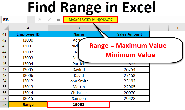
A range is the collection of values spread between the Maximum value and the Minimum value. A range is a difference between the Largest (maximum) value and the Shortest (minimum) value in a given dataset in mathematical terms.
Range defines the spread of values in any dataset. It calculates by a simple formula like below:
Range = Maximum Value – Minimum Value
How to Find Range in Excel?
Finding a range is a very simple process, and it is calculated using the Excel in-built functions MAX and MIN. Let’s understand the working of finding a range in excel with some examples.
You can download this Find Range Excel Template here – Find Range Excel Template
Range in Excel – Example #1
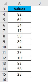
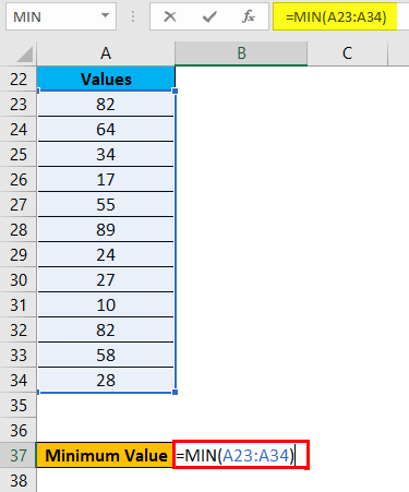
We have given below a list of values:
23, 11, 45, 21, 2, 60, 10, 35
The largest number in the above-given range is 60, and the smallest number is 2.
Thus, the Range = 60-2 = 58
Explanation:
- In this above example, the Range is 58 in the given dataset, which defines the span of the dataset. It gave you a visual indication of the range as we are looking for the highest and smallest point.
- If the dataset is large, it gives you the widespread of the result.
- If the dataset is small, it gives you a closely centered result.
A process of defining the range in Excel
For defining the range, we need to find out the maximum and minimum values of the dataset. In this process, two function plays a very important role. They are:
- MAX
- MIN
Use of MAX function:
Let’s take an example to understand the usage of this function.
Range in Excel – Example #2
We have given some set of values:
For finding the maximum value from the dataset, we will apply here the MAX function as below screenshot:
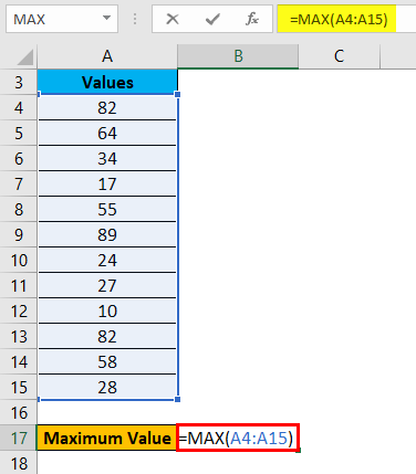
Hit enter, and it will give you the maximum value. The result is shown below:
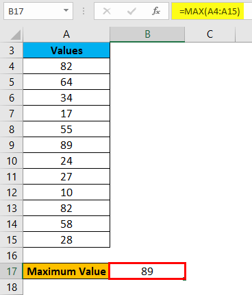
Range in Excel – Example #3
Use of MIN function:
Let’s take the same above dataset to understand the usage of this function.
For calculating the minimum value from the given dataset, we will apply the MIN function here as per the below screenshot.
Press ENTER key, and it will give you the minimum value. The result is given below:
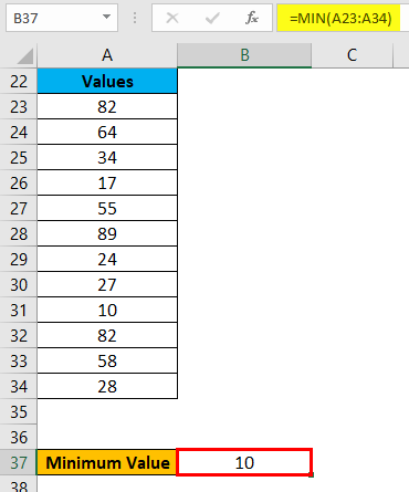
Now you can find out the range of the dataset after taking the difference between Maximum and Minimum value.
We can reduce the steps for calculating the range of a dataset by using the MAX and MIN functions together in one line.
For this, we again take an example to understand the process.
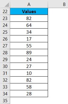
Range in Excel – Example #4
Let’s assume the below dataset of a company employee with their achieved sales target.
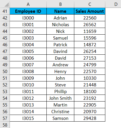
Now for identifying the span of sales amount in the above dataset, we will calculate the range. For this, we will follow the same procedure as we did in the above examples.
We will apply the MAX and MIN functions for calculating the Maximum and Minimum sales amount in the data.
For finding the range of sales amount, we will apply the below formula:
Range = Maximum Value – Minimum Value
Refer to the below screenshot:
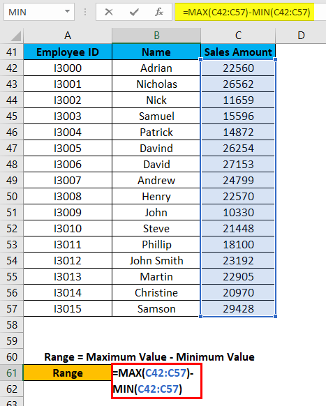
Press Enter key, and it will give you the range of the dataset. The result is shown below:
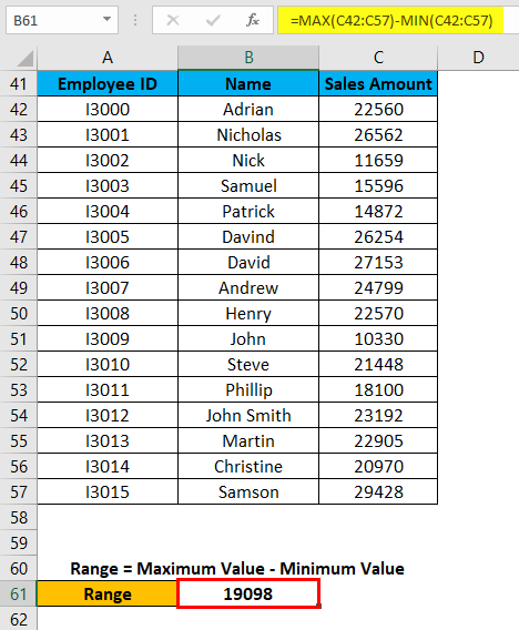
As we can see in the above screenshot, we applied the MAX and MIN formulas in one line, and by calculating their results difference, we found the range of the dataset.
Things to Remember
- If the values are available in the non-adjacent cells, you want to find out the range; you can pass the cell address individually, separated with a comma as an argument of the MAX and MIN functions.
- We can reduce the steps for calculating the range by applying MAX and MIN functions in one line. (Refer to Example 4 for your reference)
Recommended Articles
This has been a guide to Range in Excel. Here we discuss how to find Range in Excel along with excel examples and downloadable excel template. You may learn more about Excel from the following articles –
- Excel Function for Range
- Excel Named Range
- VBA Range
- VBA Selecting Range
Cell, Row, Column | Range Examples | Fill a Range | Move a Range | Copy/Paste a Range | Insert Row, Column
A range in Excel is a collection of two or more cells. This chapter gives an overview of some very important range operations.
Cell, Row, Column
Let’s start by selecting a cell, row and column.
1. To select cell C3, click on the box at the intersection of column C and row 3.
2. To select column C, click on the column C header.
3. To select row 3, click on the row 3 header.
Range Examples
A range is a collection of two or more cells.
1. To select the range B2:C4, click on cell B2 and drag it to cell C4.
2. To select a range of individual cells, hold down CTRL and click on each cell that you want to include in the range.
Fill a Range
To fill a range, execute the following steps.
1a. Enter the value 2 into cell B2.
1b. Select cell B2, click on the lower right corner of cell B2 and drag it down to cell B8.
Result:
This dragging technique is very important and you will use it very often in Excel. Here’s another example.
2a. Enter the value 2 into cell B2 and the value 4 into cell B3.
2b. Select cell B2 and cell B3, click on the lower right corner of this range and drag it down.
Excel automatically fills the range based on the pattern of the first two values. That’s pretty cool huh!? Here’s another example.
3a. Enter the date 6/13/2016 into cell B2 and the date 6/16/2016 into cell B3.
3b. Select cell B2 and cell B3, click on the lower right corner of this range and drag it down.
Note: visit our page about AutoFill for many more examples.
Move a Range
To move a range, execute the following steps.
1. Select a range and click on the border of the range.
2. Drag the range to its new location.
Copy/Paste a Range
To copy and paste a range, execute the following steps.
1. Select the range, right click, and then click Copy (or press CTRL + c).
2. Select the cell where you want the first cell of the range to appear, right click, and then click Paste under ‘Paste Options:’ (or press CTRL + v).
Insert Row, Column
To insert a row between the values 20 and 40 below, execute the following steps.
1. Select row 3.
2. Right click, and then click Insert.
Result.
The rows below the new row are shifted down. In a similar way, you can insert a column.
There is a good amount of confusion around the terms ‘Table’ and ‘Range’, especially among new Excel users.
You will find many tutorials use the terms interchangeably too.
But the two terms have some basic differences that need to be identified.
In this tutorial, we will explain what the terms Table and Range / Named range mean, how to distinguish between them, as well as how you can convert from one form to the other in Excel.
Any group of selected cells can be considered as an Excel range.
A range of cells is defined by the reference of the cell that is at the upper left corner and the one at the lower right corner.
For example, the range selected in the image below consists of cells A1 to C7, denoted as A1:C7.

An Excel range does not require cells to be contiguous. You can also add cells to a range that are away from each other.
What is an Excel Named Range?
A named range is simply a range of cells with a name.
The main purpose of using named ranges is to make references to a group of cells more intuitive.
For example, if the name of the following selected range is “Sales”, then you can simply refer to this range by name in formulas (rather than using cell references like B2:B7):

To convert a range of cells to a named range, all you need to do is select the range, type the name into the Name Box and press the return key.

You can identify a named range by selecting the range of cells.
If you see a name, instead of a cell reference in the name box, then the range of cells belongs to a Named range.
What is an Excel Table?
An Excel Table is a dynamic range of cells that are pre-formatted and organized.
A table comes with some additional features such as data aggregation, automatic updates, data styling, etc.
You can say that an Excel table is basically an Excel range, but with some added functionality.
Like named ranges, Excel tables help group a set of related cells together, with a given name.
However, they also help users clearly see the grouping through some extra styling.
As Excel is releasing new data analysis features such as Power Query, Power Pivot, and Power BI, Excel Table has become even more important. Since it’s more structured, most of these new functionalities will require you to convert your data/range into an Excel Table.
How to Identify a Table in Excel?
You can easily identify a table in Excel thanks to its distinguishable features:
- You will find filter arrows next to each column header.

- Column headings remain frozen even as you scroll down the table rows.
- The table is enclosed in a distinguishable box.

- You will also find the table styled differently from the rest of the worksheet. For example you might find rows of the table styled in alternating colors for easy viewing.
- When you click on the table (or select any cell within the table), you should see a Design tab in the main menu.

- When you click on the Design tab, you should see the name of the table on the left side of the menu ribbon.

What’s the Difference Between an Excel Table and Range?
From the first glance, it is quite easy to differentiate between a table and a range.
Not only do they look different, they are also quite different in the amount of functionality they offer.
Here are some of the differences between an Excel Table and Range:
- Cells in an Excel table need to exist as a contiguous collection of cells. Cells in a range, however, don’t necessarily need to be contiguous.
- Every column in an Excel table must have a heading (even if you choose to turn the heading row of the table off). Named ranges, on the other hand, have no such compulsion.
- Each column header (if displayed) includes filter arrows by default. These let you filter or sort the table as required. To filter or sort a range, you need to explicitly turn the filter on.
- New rows added to the table remain a part of the table. However, new rows added to a range or are not implicitly part of the original range.
- In tables, you can easily add aggregation functions (like sum, average, etc.) for each column without the need to write any formulas. With ranges, you need to explicitly add whatever formulas you need to apply.

- In order to make formulas easier to read, cells in a table can be referenced using a shorthand (also known as a structured reference). This means that instead of specifying cell references in a formula (as in ranges), you can use a shorthand as follows:
=[@Qty]*[@Sales]

- Moreover, in a table, typing the formula for one row is enough. The formula gets automatically copied to the rest of the rows in the table. In a range or named range, however, you need to use the fill handle to copy a formula down to other rows in a column.
- Adding a new row to the bottom of a table automatically copies formulae to the new row. With ranges, however, you need to use the fill handle to copy the formula every time you insert a new row.
- Pivot tables and charts that are based on a table get automatically updated with the table. This is not the case with cell ranges.
How to Convert a Range to a Table
Converting an Excel range to a table is really easy.
Let’s say you have the following range of cells and you want to convert it to a table:

Here are the steps that you need to follow to convert the range into a table:
- Select the range or click on any cell in your range.
- From the Home tab, click on ‘Format as Table’ (under the Styles group).

- You should now see a dropdown menu with a number of styling options. Select the styling option that you want to apply to your table. We selected the option highlighted below:

- This will open the ‘Format as Table’ dialog box.
- Make sure that the range displayed under ‘where is the data for your table’ is correct.

- You should see a dashed box around the cells that will be part of your table.

- If your dataset has headers, ensure that the checkbox next to ‘My table has headers’ is checked.

- Click OK.
Here’s what your table should look like if you’ve followed the above steps:

Note: Alternatively, you could use the keyboard shortcut CTRL+T in place of steps 2 and 3.
How to Convert a Table to Range
It is also possible to reverse the conversion, in other words, convert a table back into a range of cells. Here are the steps that you need to follow:
- Select any cell in your table.
- You should see a new ribbon titled ‘Table Tools’ in the main menu. Select the Design tab under this menu.

- In the Tools group, select the ‘Convert to Range’ button.

- You will be asked to confirm if you want to convert the table to a normal range. Click Yes.

Alternatively, you could simply right-click on the table and select Table->Convert to Range from the context menu that appears.

You will now find that the table features (like filter arrows and structured references in all the formulas) are no longer there since it’s now just a regular range of cells. Structured references have all turned back into regular cell references.

In this tutorial, we explained with examples how ranges and named ranges differ from tables.
To conclude, a table can be considered as a named range, but with some added functionality, like styling, easy aggregations, structured references, and more.
We hope we have been successful in clearing any confusion you might have had about ranges, named ranges, and tables.
Other Excel Tutorials you may also like:
- How to Save an Excel Table as Image
- How to Add a Total Row in Excel Table
- How to Find Range in Excel
- SUMPRODUCT vs SUMIFS Function in Excel
- How to Paste in a Filtered Column Skipping the Hidden Cells
- How to Group by Months in Excel Pivot Table?
- How to Remove Table Formatting in Excel?
- How to Rename a Table in Excel?
- Row vs Column in Excel – What’s the Difference?
На чтение 18 мин. Просмотров 75.3k.

сэр Артур Конан Дойл
Это большая ошибка — теоретизировать, прежде чем кто-то получит данные
Эта статья охватывает все, что вам нужно знать об использовании ячеек и диапазонов в VBA. Вы можете прочитать его от начала до конца, так как он сложен в логическом порядке. Или использовать оглавление ниже, чтобы перейти к разделу по вашему выбору.
Рассматриваемые темы включают свойство смещения, чтение
значений между ячейками, чтение значений в массивы и форматирование ячеек.
Содержание
- Краткое руководство по диапазонам и клеткам
- Введение
- Важное замечание
- Свойство Range
- Свойство Cells рабочего листа
- Использование Cells и Range вместе
- Свойство Offset диапазона
- Использование диапазона CurrentRegion
- Использование Rows и Columns в качестве Ranges
- Использование Range вместо Worksheet
- Чтение значений из одной ячейки в другую
- Использование метода Range.Resize
- Чтение Value в переменные
- Как копировать и вставлять ячейки
- Чтение диапазона ячеек в массив
- Пройти через все клетки в диапазоне
- Форматирование ячеек
- Основные моменты
Краткое руководство по диапазонам и клеткам
| Функция | Принимает | Возвращает | Пример | Вид |
| Range | адреса ячеек |
диапазон ячеек |
.Range(«A1:A4») | $A$1:$A$4 |
| Cells | строка, столбец |
одна ячейка |
.Cells(1,5) | $E$1 |
| Offset | строка, столбец |
диапазон | .Range(«A1:A2») .Offset(1,2) |
$C$2:$C$3 |
| Rows | строка (-и) | одна или несколько строк |
.Rows(4) .Rows(«2:4») |
$4:$4 $2:$4 |
| Columns | столбец (-цы) |
один или несколько столбцов |
.Columns(4) .Columns(«B:D») |
$D:$D $B:$D |
Введение
Это третья статья, посвященная трем основным элементам VBA. Этими тремя элементами являются Workbooks, Worksheets и Ranges/Cells. Cells, безусловно, самая важная часть Excel. Почти все, что вы делаете в Excel, начинается и заканчивается ячейками.
Вы делаете три основных вещи с помощью ячеек:
- Читаете из ячейки.
- Пишите в ячейку.
- Изменяете формат ячейки.
В Excel есть несколько методов для доступа к ячейкам, таких как Range, Cells и Offset. Можно запутаться, так как эти функции делают похожие операции.
В этой статье я расскажу о каждом из них, объясню, почему они вам нужны, и когда вам следует их использовать.
Давайте начнем с самого простого метода доступа к ячейкам — с помощью свойства Range рабочего листа.
Важное замечание
Я недавно обновил эту статью, сейчас использую Value2.
Вам может быть интересно, в чем разница между Value, Value2 и значением по умолчанию:
' Value2
Range("A1").Value2 = 56

' Value
Range("A1").Value = 56

' По умолчанию используется значение
Range("A1") = 56
Использование Value может усечь число, если ячейка отформатирована, как валюта. Если вы не используете какое-либо свойство, по умолчанию используется Value.
Лучше использовать Value2, поскольку он всегда будет возвращать фактическое значение ячейки.
Свойство Range
Рабочий лист имеет свойство Range, которое можно использовать для доступа к ячейкам в VBA. Свойство Range принимает тот же аргумент, что и большинство функций Excel Worksheet, например: «А1», «А3: С6» и т.д.
В следующем примере показано, как поместить значение в ячейку с помощью свойства Range.
Sub ZapisVYacheiku()

    ' Запишите число в ячейку A1 на листе 1 этой книги
    ThisWorkbook.Worksheets("Лист1").Range("A1").Value2 = 67

    ' Напишите текст в ячейку A2 на листе 1 этой рабочей книги
    ThisWorkbook.Worksheets("Лист1").Range("A2").Value2 = "Иван Петров"

    ' Запишите дату в ячейку A3 на листе 1 этой книги
    ThisWorkbook.Worksheets("Лист1").Range("A3").Value2 = #11/21/2019#

End Sub
Как видно из кода, Range является членом Worksheets, которая, в свою очередь, является членом Workbook. Иерархия такая же, как и в Excel, поэтому должно быть легко понять. Чтобы сделать что-то с Range, вы должны сначала указать рабочую книгу и рабочий лист, которому она принадлежит.
В оставшейся части этой статьи я буду использовать кодовое имя для ссылки на лист.

Следующий код показывает приведенный выше пример с использованием кодового имени рабочего листа, т.е. Лист1 вместо ThisWorkbook.Worksheets («Лист1»).
Sub IspKodImya ()

    ' Запишите число в ячейку A1 на листе 1 этой книги
     Sheet1.Range("A1").Value2 = 67

    ' Напишите текст в ячейку A2 на листе 1 этой рабочей книги
    Sheet1.Range("A2").Value2 = "Иван Петров"

    ' Запишите дату в ячейку A3 на листе 1 этой книги
    Sheet1.Range("A3").Value2 = #11/21/2019#

End Sub
Вы также можете писать в несколько ячеек, используя свойство
Range
Sub ZapisNeskol()

    ' Запишите число в диапазон ячеек
    Sheet1.Range("A1:A10").Value2 = 67

    ' Написать текст в несколько диапазонов ячеек
    Sheet1.Range("B2:B5,B7:B9").Value2 = "Иван Петров"

End Sub
Свойство Cells рабочего листа
У Объекта листа есть другое свойство, называемое Cells, которое очень похоже на Range . Есть два отличия:
- Cells возвращают диапазон только одной ячейки.
- Cells принимает строку и столбец в качестве аргументов.
В приведенном ниже примере показано, как записывать значения
в ячейки, используя свойства Range и Cells.
Sub IspCells()

    ' Написать в А1
    Sheet1.Range("A1").Value2 = 10
    Sheet1.Cells(1, 1).Value2  = 10

    ' Написать в А10
    Sheet1.Range("A10").Value2 = 10
    Sheet1.Cells(10, 1).Value2  = 10

    ' Написать в E1
    Sheet1.Range("E1").Value2 = 10
    Sheet1.Cells(1, 5).Value2  = 10

End Sub
Вам должно быть интересно, когда использовать Cells, а когда Range. Использование Range полезно для доступа к одним и тем же ячейкам при каждом запуске макроса.
Например, если вы использовали макрос для вычисления суммы и
каждый раз записывали ее в ячейку A10, тогда Range подойдет для этой задачи.
Использование свойства Cells полезно, если вы обращаетесь к
ячейке по номеру, который может отличаться. Проще объяснить это на примере.
В следующем коде мы просим пользователя указать номер столбца. Использование Cells дает нам возможность использовать переменное число для столбца.
Sub ZapisVPervuyuPustuyuYacheiku()

    Dim UserCol As Integer

    ' Получить номер столбца от пользователя
    UserCol = Application.InputBox("Пожалуйста, введите номер столбца...", Type:=1)

    ' Написать текст в выбранный пользователем столбец
    Sheet1.Cells(1, UserCol).Value2 = "Иван Петров"

End Sub
В приведенном выше примере мы используем номер для столбца,
а не букву.
Чтобы использовать Range здесь, потребуется преобразовать эти значения в ссылку на
буквенно-цифровую ячейку, например, «С1». Использование свойства Cells позволяет нам
предоставить строку и номер столбца для доступа к ячейке.
Иногда вам может понадобиться вернуть более одной ячейки, используя номера строк и столбцов. В следующем разделе показано, как это сделать.
Использование Cells и Range вместе
Как вы уже видели, вы можете получить доступ только к одной ячейке, используя свойство Cells. Если вы хотите вернуть диапазон ячеек, вы можете использовать Cells с Range следующим образом:
Sub IspCellsSRange()

    With Sheet1
        ' Запишите 5 в диапазон A1: A10, используя свойство Cells
        .Range(.Cells(1, 1), .Cells(10, 1)).Value2 = 5

        ' Диапазон B1: Z1 будет выделен жирным шрифтом
        .Range(.Cells(1, 2), .Cells(1, 26)).Font.Bold = True

    End With

End Sub
Как видите, вы предоставляете начальную и конечную ячейку
диапазона. Иногда бывает сложно увидеть, с каким диапазоном вы имеете дело,
когда значением являются все числа. Range имеет свойство Address, которое
отображает буквенно-цифровую ячейку для любого диапазона. Это может
пригодиться, когда вы впервые отлаживаете или пишете код.
В следующем примере мы распечатываем адрес используемых нами
диапазонов.
Sub PokazatAdresDiapazona()

    ' Примечание. Использование подчеркивания позволяет разделить строки кода.
    With Sheet1

        ' Запишите 5 в диапазон A1: A10, используя свойство Cells
        .Range(.Cells(1, 1), .Cells(10, 1)).Value2 = 5
        Debug.Print "Первый адрес: " _
            + .Range(.Cells(1, 1), .Cells(10, 1)).Address

        ' Диапазон B1: Z1 будет выделен жирным шрифтом
        .Range(.Cells(1, 2), .Cells(1, 26)).Font.Bold = True
        Debug.Print "Второй адрес : " _
            + .Range(.Cells(1, 2), .Cells(1, 26)).Address

    End With

End Sub
В примере я использовал Debug.Print для печати в Immediate Window. Для просмотра этого окна выберите «View» -> «в Immediate Window» (Ctrl + G).


Свойство Offset диапазона
У диапазона есть свойство, которое называется Offset. Термин «Offset» относится к отсчету от исходной позиции. Он часто используется в определенных областях программирования. С помощью свойства «Offset» вы можете получить диапазон ячеек того же размера и на определенном расстоянии от текущего диапазона. Это полезно, потому что иногда вы можете выбрать диапазон на основе определенного условия. Например, на скриншоте ниже есть столбец для каждого дня недели. Учитывая номер дня (т.е. понедельник = 1, вторник = 2 и т.д.). Нам нужно записать значение в правильный столбец.

Сначала мы попытаемся сделать это без использования Offset.
' Это Sub тесты с разными значениями
Sub TestSelect()

    ' Понедельник
    SetValueSelect 1, 111.21
    ' Среда
    SetValueSelect 3, 456.99
    ' Пятница
    SetValueSelect 5, 432.25
    ' Воскресение
    SetValueSelect 7, 710.17

End Sub

' Записывает значение в столбец на основе дня
Public Sub SetValueSelect(lDay As Long, lValue As Currency)

    Select Case lDay
        Case 1: Sheet1.Range("H3").Value2 = lValue
        Case 2: Sheet1.Range("I3").Value2 = lValue
        Case 3: Sheet1.Range("J3").Value2 = lValue
        Case 4: Sheet1.Range("K3").Value2 = lValue
        Case 5: Sheet1.Range("L3").Value2 = lValue
        Case 6: Sheet1.Range("M3").Value2 = lValue
        Case 7: Sheet1.Range("N3").Value2 = lValue
    End Select

End Sub
Как видно из примера, нам нужно добавить строку для каждого возможного варианта. Это не идеальная ситуация. Использование свойства Offset обеспечивает более чистое решение.
' Это Sub тесты с разными значениями
Sub TestOffset()

    DayOffSet 1, 111.01
    DayOffSet 3, 456.99
    DayOffSet 5, 432.25
    DayOffSet 7, 710.17

End Sub

Public Sub DayOffSet(lDay As Long, lValue As Currency)

    ' Мы используем значение дня с Offset, чтобы указать правильный столбец
    Sheet1.Range("G3").Offset(, lDay).Value2 = lValue

End Sub
Как видите, это решение намного лучше. Если количество дней увеличилось, нам больше не нужно добавлять код. Чтобы Offset был полезен, должна быть какая-то связь между позициями ячеек. Если столбцы Day в приведенном выше примере были случайными, мы не могли бы использовать Offset. Мы должны были бы использовать первое решение.
Следует иметь в виду, что Offset сохраняет размер диапазона. Итак .Range («A1:A3»).Offset (1,1) возвращает диапазон B2:B4. Ниже приведены еще несколько примеров использования Offset.
Sub IspOffset()

    ' Запись в В2 - без Offset
    Sheet1.Range("B2").Offset().Value2 = "Ячейка B2"

    ' Написать в C2 - 1 столбец справа
    Sheet1.Range("B2").Offset(, 1).Value2 = "Ячейка C2"

    ' Написать в B3 - 1 строка вниз
    Sheet1.Range("B2").Offset(1).Value2 = "Ячейка B3"

    ' Запись в C3 - 1 столбец справа и 1 строка вниз
    Sheet1.Range("B2").Offset(1, 1).Value2 = "Ячейка C3"

    ' Написать в A1 - 1 столбец слева и 1 строка вверх
    Sheet1.Range("B2").Offset(-1, -1).Value2 = "Ячейка A1"

    ' Запись в диапазон E3: G13 - 1 столбец справа и 1 строка вниз
    Sheet1.Range("D2:F12").Offset(1, 1).Value2 = "Ячейки E3:G13"

End Sub
Использование диапазона CurrentRegion
CurrentRegion возвращает диапазон всех соседних ячеек в данный диапазон. На скриншоте ниже вы можете увидеть два CurrentRegion. Я добавил границы, чтобы прояснить CurrentRegion.

Строка или столбец пустых ячеек означает конец CurrentRegion.
Вы можете вручную проверить
CurrentRegion в Excel, выбрав диапазон и нажав Ctrl + Shift + *.
Если мы возьмем любой диапазон
ячеек в пределах границы и применим CurrentRegion, мы вернем диапазон ячеек во
всей области.
Например:
Range («B3»). CurrentRegion вернет диапазон B3:D14
Range («D14»). CurrentRegion вернет диапазон B3:D14
Range («C8:C9»). CurrentRegion вернет диапазон B3:D14 и так далее
Как пользоваться
Мы получаем CurrentRegion следующим образом
' CurrentRegion вернет B3:D14 из приведенного выше примера
Dim rg As Range
Set rg = Sheet1.Range("B3").CurrentRegion
Только чтение строк данных
Прочитать диапазон из второй строки, т.е. пропустить строку заголовка.
' CurrentRegion вернет B3:D14 из приведенного выше примера
Dim rg As Range
Set rg = Sheet1.Range("B3").CurrentRegion

' Начало в строке 2 - строка после заголовка
Dim i As Long
For i = 2 To rg.Rows.Count
    ' текущая строка, столбец 1 диапазона
    Debug.Print rg.Cells(i, 1).Value2
Next i
Удалить заголовок
Удалить строку заголовка (т.е. первую строку) из диапазона. Например, если диапазон — A1:D4, это возвратит A2:D4
' CurrentRegion вернет B3:D14 из приведенного выше примера
Dim rg As Range
Set rg = Sheet1.Range("B3").CurrentRegion

' Удалить заголовок
Set rg = rg.Resize(rg.Rows.Count - 1).Offset(1)

' Начните со строки 1, так как нет строки заголовка
Dim i As Long
For i = 1 To rg.Rows.Count
    ' текущая строка, столбец 1 диапазона
    Debug.Print rg.Cells(i, 1).Value2
Next i
Использование Rows и Columns в качестве Ranges
Если вы хотите что-то сделать со всей строкой или столбцом,
вы можете использовать свойство «Rows и
Columns» на рабочем листе. Они оба принимают один параметр — номер строки
или столбца, к которому вы хотите получить доступ.
Sub IspRowIColumns()

    ' Установите размер шрифта столбца B на 9
    Sheet1.Columns(2).Font.Size = 9

    ' Установите ширину столбцов от D до F
    Sheet1.Columns("D:F").ColumnWidth = 4

    ' Установите размер шрифта строки 5 до 18
    Sheet1.Rows(5).Font.Size = 18

End Sub
Использование Range вместо Worksheet
Вы также можете использовать Cella, Rows и Columns, как часть Range, а не как часть Worksheet. У вас может быть особая необходимость в этом, но в противном случае я бы избегал практики. Это делает код более сложным. Простой код — твой друг. Это уменьшает вероятность ошибок.
Код ниже выделит второй столбец диапазона полужирным. Поскольку диапазон имеет только две строки, весь столбец считается B1:B2
Sub IspColumnsVRange()

    ' Это выделит B1 и B2 жирным шрифтом.
    Sheet1.Range("A1:C2").Columns(2).Font.Bold = True

End Sub
Чтение значений из одной ячейки в другую
В большинстве примеров мы записали значения в ячейку. Мы
делаем это, помещая диапазон слева от знака равенства и значение для размещения
в ячейке справа. Для записи данных из одной ячейки в другую мы делаем то же
самое. Диапазон назначения идет слева, а диапазон источника — справа.
В следующем примере показано, как это сделать:
Sub ChitatZnacheniya()

    ' Поместите значение из B1 в A1
    Sheet1.Range("A1").Value2 = Sheet1.Range("B1").Value2

    ' Поместите значение из B3 в лист2 в ячейку A1
    Sheet1.Range("A1").Value2 = Sheet2.Range("B3").Value2

    ' Поместите значение от B1 в ячейки A1 до A5
    Sheet1.Range("A1:A5").Value2 = Sheet1.Range("B1").Value2

    ' Вам необходимо использовать свойство «Value», чтобы прочитать несколько ячеек
    Sheet1.Range("A1:A5").Value2 = Sheet1.Range("B1:B5").Value2

End Sub
Как видно из этого примера, невозможно читать из нескольких ячеек. Если вы хотите сделать это, вы можете использовать функцию копирования Range с параметром Destination.
Sub KopirovatZnacheniya()

    ' Сохранить диапазон копирования в переменной
    Dim rgCopy As Range
    Set rgCopy = Sheet1.Range("B1:B5")

    ' Используйте это для копирования из более чем одной ячейки
    rgCopy.Copy Destination:=Sheet1.Range("A1:A5")

    ' Вы можете вставить в несколько мест назначения
    rgCopy.Copy Destination:=Sheet1.Range("A1:A5,C2:C6")

End Sub
Функция Copy копирует все, включая формат ячеек. Это тот же результат, что и ручное копирование и вставка выделения. Подробнее об этом вы можете узнать в разделе «Копирование и вставка ячеек»
Использование метода Range.Resize
При копировании из одного диапазона в другой с использованием присваивания (т.е. знака равенства) диапазон назначения должен быть того же размера, что и исходный диапазон.
Использование функции Resize позволяет изменить размер
диапазона до заданного количества строк и столбцов.
Например:
Sub ResizePrimeri()

    ' Печатает А1
    Debug.Print Sheet1.Range("A1").Address

    ' Печатает A1:A2
    Debug.Print Sheet1.Range("A1").Resize(2, 1).Address

    ' Печатает A1:A5
    Debug.Print Sheet1.Range("A1").Resize(5, 1).Address

    ' Печатает A1:D1
    Debug.Print Sheet1.Range("A1").Resize(1, 4).Address

    ' Печатает A1:C3
    Debug.Print Sheet1.Range("A1").Resize(3, 3).Address

End Sub
Когда мы хотим изменить наш целевой диапазон, мы можем
просто использовать исходный размер диапазона.
Другими словами, мы используем количество строк и столбцов
исходного диапазона в качестве параметров для изменения размера:
Sub Resize()

    Dim rgSrc As Range, rgDest As Range

    ' Получить все данные в текущей области
    Set rgSrc = Sheet1.Range("A1").CurrentRegion

      ' Получить диапазон назначения
    Set rgDest = Sheet2.Range("A1")
    Set rgDest = rgDest.Resize(rgSrc.Rows.Count, rgSrc.Columns.Count)

    rgDest.Value2 = rgSrc.Value2

End Sub
Мы можем сделать изменение размера в одну строку, если нужно:
Sub Resize2()

    Dim rgSrc As Range

    ' Получить все данные в ткущей области
    Set rgSrc = Sheet1.Range("A1").CurrentRegion

    With rgSrc
        Sheet2.Range("A1").Resize(.Rows.Count, .Columns.Count) = .Value2
    End With

End Sub
Чтение Value в переменные
Мы рассмотрели, как читать из одной клетки в другую. Вы также можете читать из ячейки в переменную. Переменная используется для хранения значений во время работы макроса. Обычно вы делаете это, когда хотите манипулировать данными перед тем, как их записать. Ниже приведен простой пример использования переменной. Как видите, значение элемента справа от равенства записывается в элементе слева от равенства.
Sub IspVar()

    ' Создайте
    Dim val As Integer

    ' Читать число из ячейки
    val = Sheet1.Range("A1").Value2

    ' Добавить 1 к значению
    val = val + 1

    ' Запишите новое значение в ячейку
    Sheet1.Range("A2").Value2 = val

End Sub
Для чтения текста в переменную вы используете переменную
типа String.
Sub IspVarText()

    ' Объявите переменную типа string
    Dim sText As String

    ' Считать значение из ячейки
    sText = Sheet1.Range("A1").Value2

    ' Записать значение в ячейку
    Sheet1.Range("A2").Value2 = sText

End Sub
Вы можете записать переменную в диапазон ячеек. Вы просто
указываете диапазон слева, и значение будет записано во все ячейки диапазона.
Sub VarNeskol()

    ' Считать значение из ячейки
    Sheet1.Range("A1:B10").Value2 = 66

End Sub
Вы не можете читать из нескольких ячеек в переменную. Однако
вы можете читать массив, который представляет собой набор переменных. Мы
рассмотрим это в следующем разделе.
Как копировать и вставлять ячейки
Если вы хотите скопировать и вставить диапазон ячеек, вам не
нужно выбирать их. Это распространенная ошибка, допущенная новыми пользователями
VBA.
Вы можете просто скопировать ряд ячеек, как здесь:
Range("A1:B4").Copy Destination:=Range("C5")
При использовании этого метода копируется все — значения,
форматы, формулы и так далее. Если вы хотите скопировать отдельные элементы, вы
можете использовать свойство PasteSpecial
диапазона.
Работает так:
Range("A1:B4").Copy
Range("F3").PasteSpecial Paste:=xlPasteValues
Range("F3").PasteSpecial Paste:=xlPasteFormats
Range("F3").PasteSpecial Paste:=xlPasteFormulas
В следующей таблице приведен полный список всех типов вставок.
| Виды вставок |
| xlPasteAll |
| xlPasteAllExceptBorders |
| xlPasteAllMergingConditionalFormats |
| xlPasteAllUsingSourceTheme |
| xlPasteColumnWidths |
| xlPasteComments |
| xlPasteFormats |
| xlPasteFormulas |
| xlPasteFormulasAndNumberFormats |
| xlPasteValidation |
| xlPasteValues |
| xlPasteValuesAndNumberFormats |
Чтение диапазона ячеек в массив
Вы также можете скопировать значения, присвоив значение
одного диапазона другому.
Range("A3:Z3").Value2 = Range("A1:Z1").Value2
Значение диапазона в этом примере считается вариантом массива. Это означает, что вы можете легко читать из диапазона ячеек в массив. Вы также можете писать из массива в диапазон ячеек. Если вы не знакомы с массивами, вы можете проверить их в этой статье.
В следующем коде показан пример использования массива с
диапазоном.
Sub ChitatMassiv()

    ' Создать динамический массив
    Dim StudentMarks() As Variant

    ' Считать 26 значений в массив из первой строки
    StudentMarks = Range("A1:Z1").Value2

    ' Сделайте что-нибудь с массивом здесь

    ' Запишите 26 значений в третью строку
    Range("A3:Z3").Value2 = StudentMarks

End Sub
Имейте в виду, что массив, созданный для чтения, является
двумерным массивом. Это связано с тем, что электронная таблица хранит значения
в двух измерениях, то есть в строках и столбцах.
Пройти через все клетки в диапазоне
Иногда вам нужно просмотреть каждую ячейку, чтобы проверить значение.
Вы можете сделать это, используя цикл For Each, показанный в следующем коде.
Sub PeremeschatsyaPoYacheikam()

    ' Пройдите через каждую ячейку в диапазоне
    Dim rg As Range
    For Each rg In Sheet1.Range("A1:A10,A20")
        ' Распечатать адрес ячеек, которые являются отрицательными
        If rg.Value < 0 Then
            Debug.Print rg.Address + " Отрицательно."
        End If
    Next

End Sub
Вы также можете проходить последовательные ячейки, используя
свойство Cells и стандартный цикл For.
Стандартный цикл более гибок в отношении используемого вами
порядка, но он медленнее, чем цикл For Each.
Sub PerehodPoYacheikam()

    ' Пройдите клетки от А1 до А10
    Dim i As Long
    For i = 1 To 10
        ' Распечатать адрес ячеек, которые являются отрицательными
        If Range("A" & i).Value < 0 Then
            Debug.Print Range("A" & i).Address + " Отрицательно."
        End If
    Next

    ' Пройдите в обратном порядке, то есть от A10 до A1
    For i = 10 To 1 Step -1
        ' Распечатать адрес ячеек, которые являются отрицательными
        If Range("A" & i) < 0 Then
            Debug.Print Range("A" & i).Address + " Отрицательно."
        End If
    Next

End Sub
Форматирование ячеек
Иногда вам нужно будет отформатировать ячейки в электронной
таблице. Это на самом деле очень просто. В следующем примере показаны различные
форматы, которые можно добавить в любой диапазон ячеек.
Sub FormatirovanieYacheek()

    With Sheet1

        ' Форматировать шрифт
        .Range("A1").Font.Bold = True
        .Range("A1").Font.Underline = True
        .Range("A1").Font.Color = rgbNavy

        ' Установите числовой формат до 2 десятичных знаков
        .Range("B2").NumberFormat = "0.00"
        ' Установите числовой формат даты
        .Range("C2").NumberFormat = "dd/mm/yyyy"
        ' Установите формат чисел на общий
        .Range("C3").NumberFormat = "Общий"
        ' Установить числовой формат текста
        .Range("C4").NumberFormat = "Текст"

        ' Установите цвет заливки ячейки
        .Range("B3").Interior.Color = rgbSandyBrown

        ' Форматировать границы
        .Range("B4").Borders.LineStyle = xlDash
        .Range("B4").Borders.Color = rgbBlueViolet

    End With

End Sub
Основные моменты
Ниже приводится краткое изложение основных моментов
- Range возвращает диапазон ячеек
- Cells возвращают только одну клетку
- Вы можете читать из одной ячейки в другую
- Вы можете читать из диапазона ячеек в другой диапазон ячеек.
- Вы можете читать значения из ячеек в переменные и наоборот.
- Вы можете читать значения из диапазонов в массивы и наоборот
- Вы можете использовать цикл For Each или For, чтобы проходить через каждую ячейку в диапазоне.
- Свойства Rows и Columns позволяют вам получить доступ к диапазону ячеек этих типов

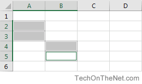
In Microsoft Excel, a range is a collection of cells. A range can be 2 or more cells and those cells don’t necessarily have to be adjacent to each other. Let’s look at some examples to quickly demonstrate the different types of ranges.
Vertical Range
This vertical range is A2:A5. In this example, if you had selected the entire column A, the range would be A:A.
Horizontal Range
This horizontal range is A2:C2. In this example, if you selected the entire row 2, the range would have be 2:2.
Mixed Range
This mixed range is A2:C5. This is a collection of cells that can be from multiple rows and columns.
Multiple Selection Range
This multiple selection range is A2:A3,B4:B5. This is a collection of cells that does not have to be adjacent.
Each range has its own set of coordinates or position in the worksheet such as A2:A5, A2:C2, A2:C5, and so on.
There are many things that you can do with ranges in Excel such as copying, moving, formatting, and naming ranges. Here is a list of topics that explain how to use ranges in Excel.
Ranges
Range is an important part of Excel because it allows you to work with selections of cells.
There are four different operations for selection;
- Selecting a cell
- Selecting multiple cells
- Selecting a column
- Selecting a row
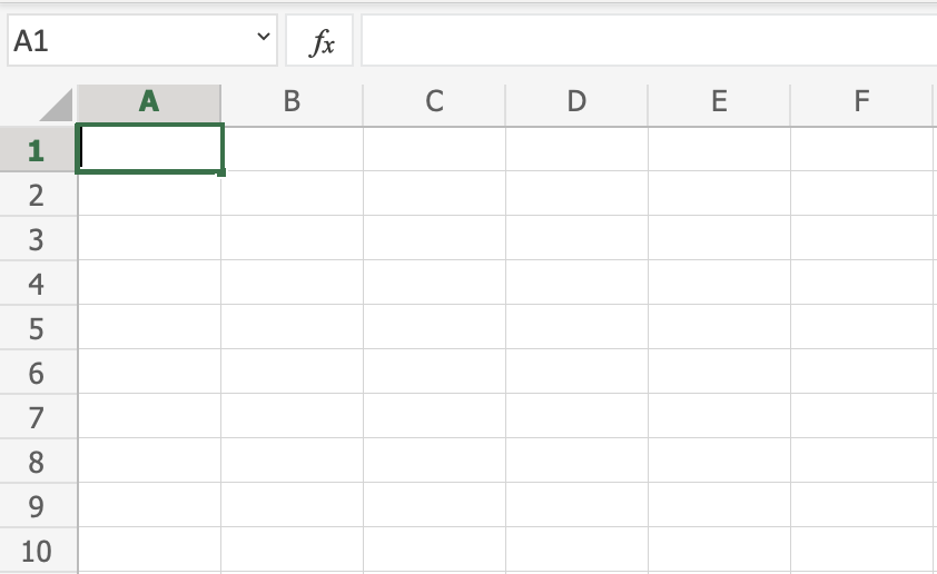
Before having a look at the different operations for selection, we will introduce the Name Box.
The Name Box
The Name Box shows you the reference of which cell or range you have selected. It can also be used to select cells or ranges by typing their values.
You will learn more about the Name Box later in this chapter.
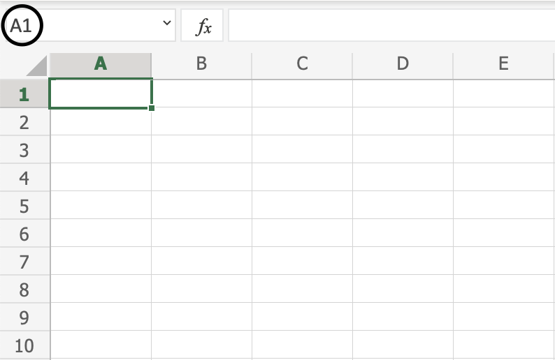
Selecting a Cell
Cells are selected by clicking them with the left mouse button or by navigating to them with the keyboard arrows.
It is easiest to use the mouse to select cells.
To select cell A1, click on it:
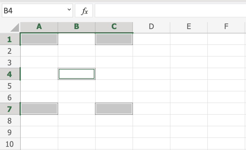
Selecting Multiple Cells
More than one cell can be selected by pressing and holding down CTRL or Command and left clicking the cells. Once finished with selecting, you can let go of CTRL or Command.
Lets try an example: Select the cells A1, A7, C1, C7 and B4.
Did it look like the picture below?
Selecting a Column
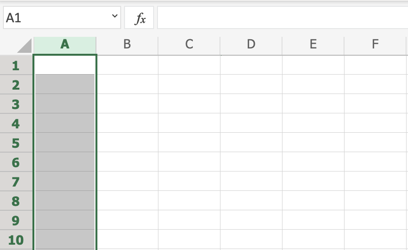
Columns are selected by left clicking it. This will select all cells in the sheet related to the column.
To select column A, click on the letter A in the column bar:
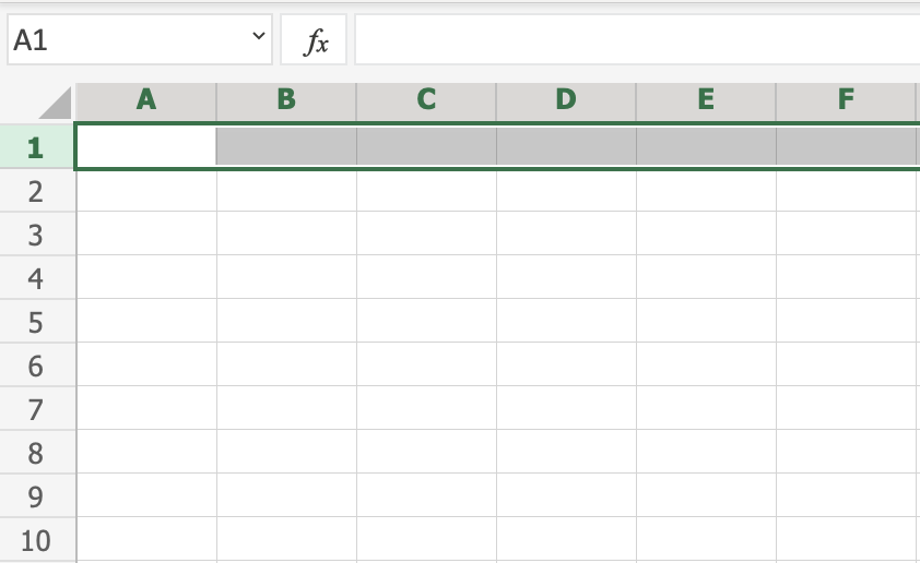
Selecting a Row
Rows are selected by left clicking it. This will select all the cells in the sheet related to that row.
To select row 1, click on its number in the row bar:
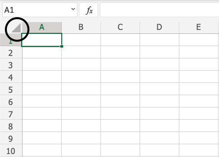
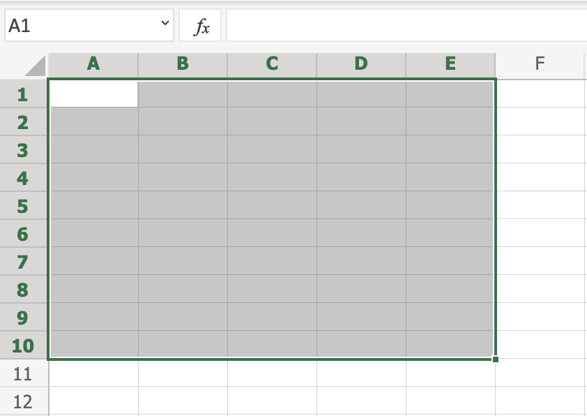
Selecting the Entire Sheet
The entire spreadsheet can be selected by clicking the triangle in the top-left corner of the spreadsheet: ![]()
Now, the whole spreadsheet is selected:
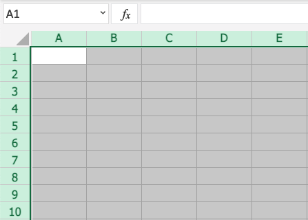
Note: You can also select the entire spreadsheet by pressing Ctrl+A for Windows, or Cmd+A for MacOS.
Selection of Ranges
Selection of cell ranges has many use areas and it is one of the most important concepts of Excel. Do not think too much about how it is used with values. You will learn about this in a later chapter. For now let’s focus on how to select ranges.
There are two ways to select a range of cells
- Name Box
- Drag to mark a range.
The easiest way is drag and mark. Let’s keep it simple and start there.
How to drag and mark a range, step-by-step:
- Select a cell
- Left click it and hold the mouse button down
- Move your mouse pointer over the range that you want selected. The range that is marked will turn grey.
- Let go of the mouse button when you have marked the range
Let’s have a look at an example for how to mark the range A1:E10.
Note: You will learn about why the range is called A1:E10 after this example.
Select cell A1:
Press and hold A1 with the left mouse button. Move to the mouse pointer to mark the selection range. The grey area helps us to see the covered range.
Let go of the left mouse button when you have marked the range A1:E10:
You have successfully selected the range A1:E10. Well done!
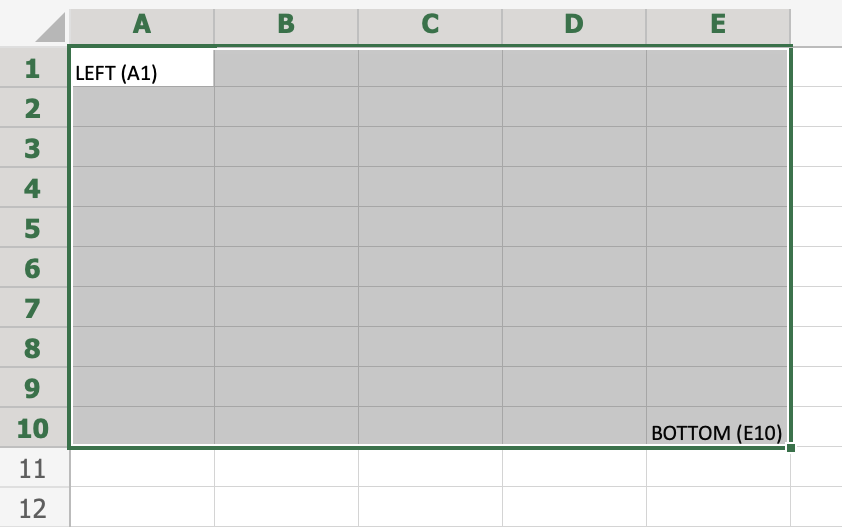
The second way to select a range is to enter the range values in the Name Box. The range is set by first entering the cell reference for the top left corner, then the bottom right corner. The range is made using those two as coordinates. That is why the cell range has the reference of two cells and the
: in between.
Top left corner reference : Right bottom corner reference
The range shown in the picture has the value of A1:E10:
The best way for now is to use the drag and mark method as it is easier and more visual.
In the next chapter you will learn about filling and how this applies to the ranges that we have just learned.
Test Yourself With Exercises
A range in Excel is nothing more than a set of adjacent cells that can be selected to perform the same operation on them. Because they are grouped, it is much easier to apply common formatting, sort items, or perform other spreadsheet tasks. Ranges are, in fact, the basis for many operations performed with the spreadsheet.
The full name of the set of cells is «range of cells», and is identified by the first and last cell in the set. For example, the range A1:C3 indicates that the two cells we have selected and on which operations can be performed are A1 and C3. We will be able to create graphs, insert functions, or form tables based on the data contained in these two cells.
To work with a range of cells, you can select them manually with the mouse, or you can type in the matrix just below the toolbar the range of cells you want to operate on following the formula above (the name of the start and end cell of the range separated by a colon).
It is worth remembering that Microsoft Excel is a software designed to work with spreadsheets. Its origins date back to 1983 when Microsoft introduced Multiplan as its own solution for this purpose. Later, when Lotus 1-2-3 was already dominating the spreadsheet market, it introduced the first version of Excel for Mac. It was 1985, and it would not be until 1987 that this software would appear for the first time in Windows. It is currently part of the Office package.