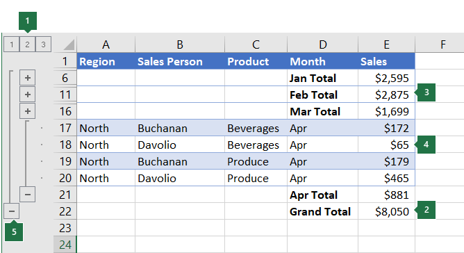
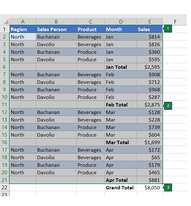
What is outlining in excel - Word и Excel - помощь в работе с программами

If you have a list of data you want to group and summarize, you can create an outline of up to eight levels. Each inner level, represented by a higher number in the outline symbols, displays detail data for the preceding outer level, represented by a lower number in the outline symbols. Use an outline to quickly display summary rows or columns, or to reveal the detail data for each group. You can create an outline of rows (as shown in the example below), an outline of columns, or an outline of both rows and columns.

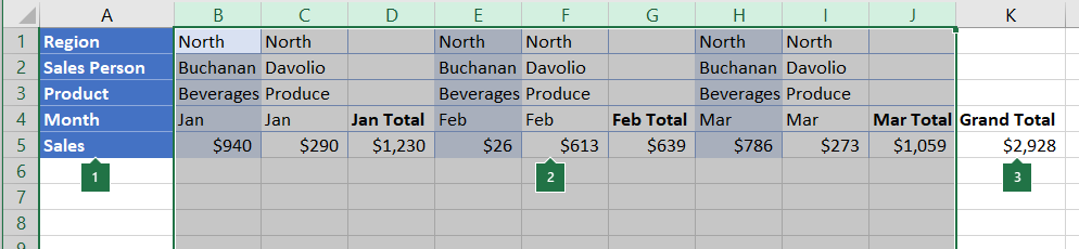
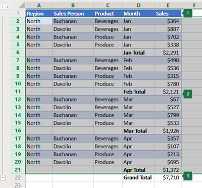
1. To display rows for a level, click the appropriate outline symbols.

2. Level 1 contains the total sales for all detail rows.

3. Level 2 contains total sales for each month in each region.

4. Level 3 contains detail rows — in this case, rows 17 through 20.

5. To expand or collapse data in your outline, click the plus and minus outline symbols, or press ALT+SHIFT+= to expand and ALT+SHIFT+- to collapse.

Make sure that each column of the data that you want to outline has a label in the first row (e.g., Region), contains similar facts in each column, and that the range you want to outline has no blank rows or columns.
If you want, your grouped detail rows can have a corresponding summary row—a subtotal. To create these, do one of the following:
- Insert summary rows by using the Subtotal command
  
  Use the Subtotal command, which inserts the SUBTOTAL function immediately below or above each group of detail rows and automatically creates the outline for you. For more information about using the Subtotal function, see SUBTOTAL function.
- Insert your own summary rows
  
  Insert your own summary rows, with formulas, immediately below or above each group of detail rows. For example, under (or above) the rows of sales data for March and April, use the SUM function to subtotal the sales for those months. The table later in this topic shows you an example of this.
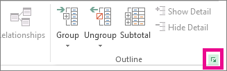
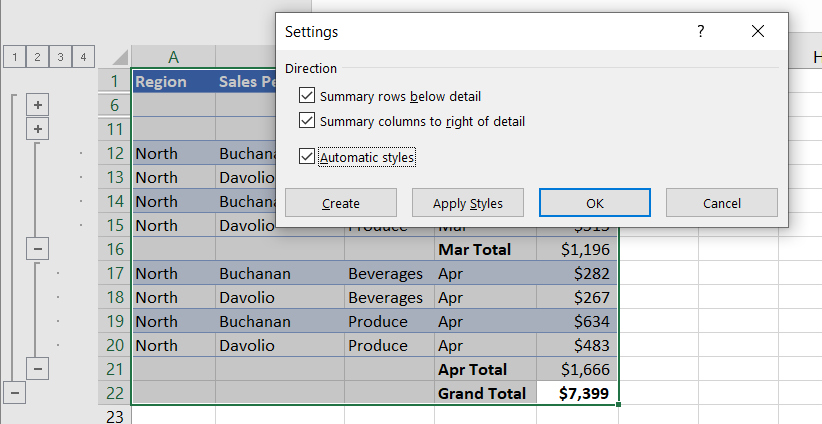
By default, Excel looks for summary rows below the details they summarize, but it’s possible to create them above the detail rows. If you created the summary rows below the details, skip to the next step (step 4). If you created your summary rows above your detail rows, on the Data tab, in the Outline group, click the dialog box launcher.

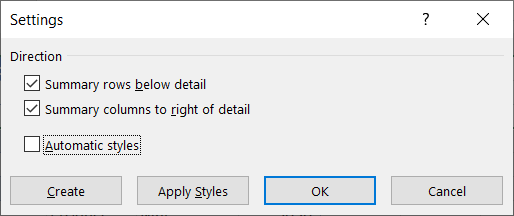
The Settings dialog box opens.

Then in the Settings dialog box, clear the Summary rows below detail checkbox, and then click OK.

Outline your data. Do one of the following:

Outline the data automatically

Select a cell in the range of cells you want to outline.
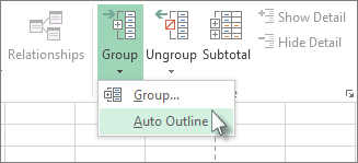
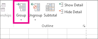
On the Data tab, in the Outline group, click the arrow under Group, and then click Auto Outline.

Outline the data manually

Important: When you manually group outline levels, it’s best to have all data displayed to avoid grouping the rows incorrectly.

To outline the outer group (level 1), select all of the rows the outer group will contain (i.e., the detail rows and if you added them, their summary rows).

1. The first row contains labels, and is not selected.

2. Since this is the outer group, select all the rows with subtotals and details.

3. Don’t select the grand total.

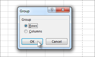
On the Data tab, in the Outline group, click Group. Then in the Group dialog box, click Rows, and then click OK.

Tip: If you select entire rows instead of just the cells, Excel automatically groups by row — the Group dialog box doesn’t even open.

The outline symbols appear beside the group on the screen.

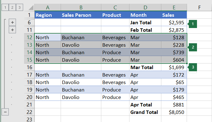
Optionally, outline an inner, nested group — the detail rows for a given section of your data.

Note: If you don’t need to create any inner groups, skip to step f, below.

For each inner, nested group, select the detail rows adjacent to the row that contains the summary row.

1. You can create multiple groups at each inner level. Here, two sections are already grouped at level 2.

2. This section is selected and ready to group.

3. Don’t select the summary row for the data you are grouping.

On the Data tab, in the Outline group, click Group.

Then in the Group dialog box, click Rows, and then click OK. The outline symbols appear beside the group on the screen.

Tip: If you select entire rows instead of just the cells, Excel automatically groups by row — the Group dialog box doesn’t even open.
Continue selecting and grouping inner rows until you have created all of the levels that you want in the outline.
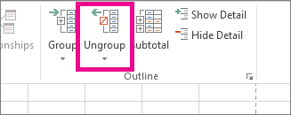
If you want to ungroup rows, select the rows, and then on the Data tab, in the Outline group, click Ungroup.

You can also ungroup sections of the outline without removing the entire level. Hold down SHIFT while you click the or for the group, and then on the Data tab, in the Outline group, click Ungroup.

Important: If you ungroup an outline while the detail data is hidden, the detail rows may remain hidden. To display the data, drag across the visible row numbers adjacent to the hidden rows. Then on the Home tab, in the Cells group, click Format, point to Hide & Unhide, and then click Unhide Rows.

Make sure that each row of the data that you want to outline has a label in the first column, contains similar facts in each row, and the range has no blank rows or columns.
Insert your own summary columns with formulas immediately to the right or left of each group of detail columns. The table listed in step 4 below shows you an example.

Note: To outline data by columns, you must have summary columns that contain formulas that reference cells in each of the detail columns for that group.
If your summary column is to the left of the detail columns, on the Data tab, in the Outline group, click the dialog box launcher.

The Settings dialog box opens.

Then in the Settings dialog box, clear the Summary columns to right of detail check box, and click OK.

To outline the data, do one of the following:

Outline the data automatically

Select a cell in the range.
On the Data tab, in the Outline group, click the arrow below Group and click Auto Outline.

Outline the data manually

Important: When you manually group outline levels, it’s best to have all data displayed to avoid grouping columns incorrectly.

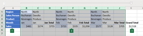
To outline the outer group (level 1), select all of the subordinate summary columns, as well as their related detail data.

1. Column A contains labels.

2. Select all the detail and subtotal columns. Note that if you don’t select entire columns, when you click Group (on the Data tab in the Outline group) the Group dialog box will open and ask you to choose Rows or Columns.

3. Don’t select the grand total column.

On the Data tab, in the Outline group, click Group.

The outline symbol appears above the group.

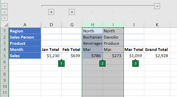
To outline an inner, nested group of detail columns (level 2 or higher), select the detail columns adjacent to the column that contains the summary column.

1. You can create multiple groups at each inner level. Here, two sections are already grouped at level 2.

2. These columns are selected and ready to group. Note that if you don’t select entire columns, when you click Group (on the Data tab in the Outline group) the Group dialog box will open and ask you to choose Rows or Columns.

3. Don’t select the summary column for the data you are grouping.

On the Data tab, in the Outline group, click Group.

The outline symbols appear beside the group on the screen.

Continue selecting and grouping inner columns until you have created all of the levels that you want in the outline.
If you want to ungroup columns, select the columns, and then on the Data tab, in the Outline group, click Ungroup.

You can also ungroup sections of the outline without removing the entire level. Hold down SHIFT while you click the or for the group, and then on the Data tab, in the Outline group, click Ungroup.

If you ungroup an outline while the detail data is hidden, the detail columns may remain hidden. To display the data, drag across the visible column letters adjacent to the hidden columns. On the Home tab, in the Cells group, click Format, point to Hide & Unhide, and then click Unhide Columns

If you don’t see the outline symbols , , and , go to File > Options > Advanced, and then under the Display options for this worksheet section, select the Show outline symbols if an outline is applied check box, and then click OK.
Do one or more of the following:
- Show or hide the detail data for a group
  
  To display the detail data within a group, click the button for the group, or press ALT+SHIFT+=.
- To hide the detail data for a group, click the button for the group, or press ALT+SHIFT+-.
- Expand or collapse the entire outline to a particular level
  
  In the outline symbols, click the number of the level that you want. Detail data at lower levels is then hidden.
  
  For example, if an outline has four levels, you can hide the fourth level while displaying the rest of the levels by clicking .
- Show or hide all of the outlined detail data
  
  To show all detail data, click the lowest level in the outline symbols. For example, if there are three levels, click .
- To hide all detail data, click .

For outlined rows, Microsoft Excel uses styles such as RowLevel_1 and RowLevel_2 . For outlined columns, Excel uses styles such as ColLevel_1 and ColLevel_2. These styles use bold, italic, and other text formats to differentiate the summary rows or columns in your data. By changing the way each of these styles is defined, you can apply different text and cell formats to customize the appearance of your outline. You can apply a style to an outline either when you create the outline or after you create it.

Do one or more of the following:

Automatically apply a style to new summary rows or columns

On the Data tab, in the Outline group, click the dialog box launcher.

The Settings dialog box opens.
Select the Automatic styles check box.

Apply a style to an existing summary row or column

Select the cells to which you want to apply a style.
On the Data tab, in the Outline group, click the dialog box launcher.

The Settings dialog box opens.
Select the Automatic styles check box, and then click Apply Styles.

You can also use autoformats to format outlined data.

If you don’t see the outline symbols , , and , go to File > Options > Advanced, and then under the Display options for this worksheet section, select the Show outline symbols if an outline is applied check box.
Use the outline symbols , , and to hide the detail data that you don’t want copied.

For more information, see the section, Show or hide outlined data.
Select the range of summary rows.
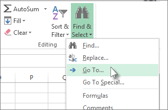
On the Home tab, in the Editing group, click Find & Select, and then click Go To.
Click Go To Special.
Click Visible cells only.
Click OK, and then copy the data.

Note: No data is deleted when you hide or remove an outline.

Hide an outline

Go to File > Options > Advanced, and then under the Display options for this worksheet section, uncheck the Show outline symbols if an outline is applied check box.

Remove an outline

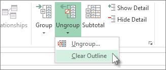
Click the worksheet.
One the Data tab, in the Outline group, click Ungroup and click Clear Outline.

Important: If you remove an outline while the detail data is hidden, the detail rows or columns may remain hidden. To display the data, drag across the visible row numbers or column letters adjacent to the hidden rows and columns. On the Home tab, in the Cells group, click Format, point to Hide & Unhide, and then click Unhide Rows or Unhide Columns.

Imagine that you want to create a summary report of your data that only displays totals accompanied by a chart of those totals. In general, you can do the following:

Create a summary report
1. Outline your data.
  
  For more information, see the sections Create an outline of rows or Create an outline of columns.
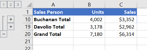
2. Hide the detail by clicking the outline symbols , , and to show only the totals as shown in the following example of a row outline:
3. For more information, see the section, Show or hide outlined data.
Chart the summary report
1. Select the summary data that you want to chart.
  
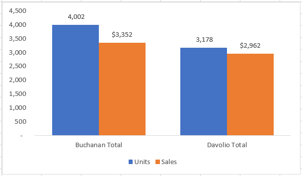
  For example, to chart only the Buchanan and Davolio totals, but not the grand totals, select cells A1 through C19 as shown in the above example.
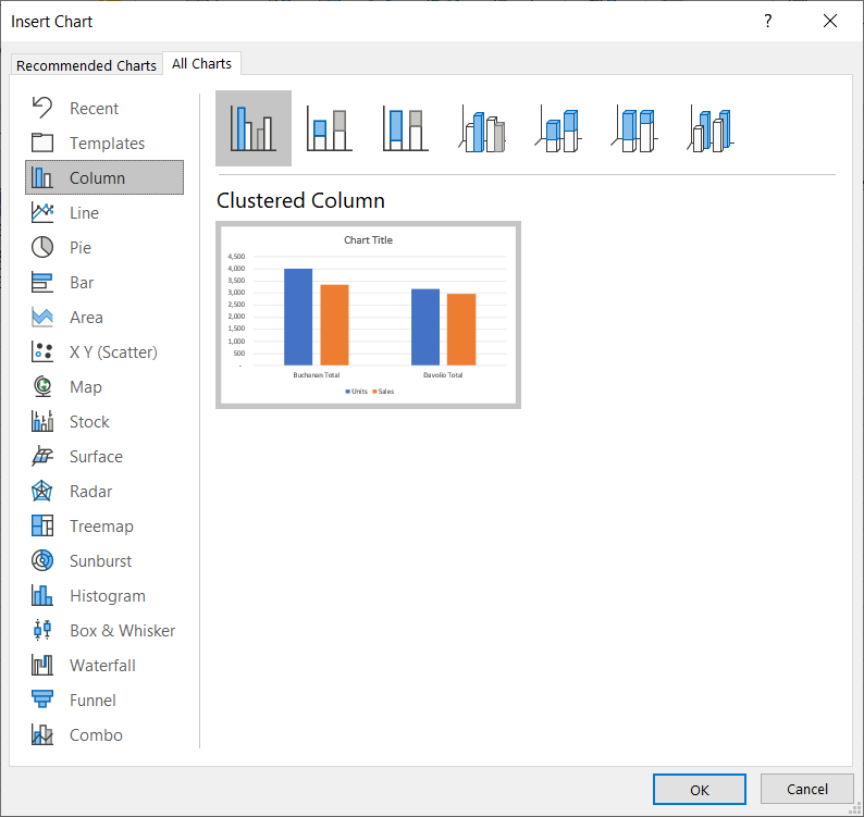
2. Click Insert > Charts > Recommended Charts, then click the All Charts tab and choose your chart type.
  
  For example, if you chose the Clustered Column option, your chart would look like this:
  
  If you show or hide details in the outlined list of data, the chart is also updated to show or hide the data.

You can group (or outline) rows and columns in Excel for the web.

Note: Although you can add summary rows or columns to your data (by using functions such as SUM or SUBTOTAL), you cannot apply styles or set a position for summary rows and columns in Excel for the web.

Create an outline of rows or columns

Outline of rows in Excel Online

The first column contains labels.
The detail rows and summary rows are grouped in the outline.
The grand total is not grouped in the outline.

Outline of columns in Excel Online

The first row contains labels.
The detail columns and summary columns are grouped in the outline.
The grand total is not grouped in the outline.

Make sure that each column (or row) of the data that you want to outline has a label in the first row (or column), contains similar facts in each column (or row), and that the range has no blank rows or columns.
Select the data (including any summary rows or columns).
On the Data tab, in the Outline group, click Group > Group Rows or Group Columns.
Optionally, if you want to outline an inner, nested group — select the rows or columns within the outlined data range, and repeat step 3.
Continue selecting and grouping inner rows or columns until you have created all of the levels that you want in the outline.

Ungroup rows or columns

To ungroup, select the rows or columns, and then on the Data tab, in the Outline group, click Ungroup and select Ungroup Rows or Ungroup Columns.

Show or hide outlined data

Do one or more of the following:

Show or hide the detail data for a group

To display the detail data within a group, click the for the group, or press ALT+SHIFT+=.
To hide the detail data for a group, click the for the group, or press ALT+SHIFT+-.

Expand or collapse the entire outline to a particular level

In the outline symbols, click the number of the level that you want. Detail data at lower levels is then hidden.
For example, if an outline has four levels, you can hide the fourth level while displaying the rest of the levels by clicking .

Show or hide all of the outlined detail data

To show all detail data, click the lowest level in the outline symbols. For example, if there are three levels, click .
To hide all detail data, click .

Need more help?

You can always ask an expert in the Excel Tech Community or get support in the Answers community.

How do I outline text in Excel?

If you are using Excel or PowerPoint
To add the same outline to text in multiple places, select the first piece of text, and then press and hold CTRL while you select the other pieces of text. To add or change an outline color, click the color that you want. To choose no color, click No Outline.

How do you make an outline on a spreadsheet?

How to Do an Outline in Excel

Drag the mouse cursor over the sheet’s cells to select its data.
Click the ribbon’s “Data” tab and click “Group” to open a pop-up menu.
Click “Group” to open the Group dialog box.
Click the “Rows” option button to collapse rows in the spreadsheet.
Click “OK” to create the outline.

How do you create an outline border in Excel?

Here’s how:

Click Home > the Borders arrow .
Pick Draw Borders for outer borders or Draw Border Grid for gridlines.
Click the Borders arrow > Line Color arrow, and then pick a color.
Click the Borders arrow > Line Style arrow, and then pick a line style.
Select cells you want to draw borders around.

Why can’t I create an outline in Excel?

If you receive a pop-up box that says “Cannot create an outline”, your data doesn’t have an outline-compatible formula in it. You’ll need to manually outline the data.

How do I make an outline?

To create an outline:

Place your thesis statement at the beginning.
List the major points that support your thesis. Label them in Roman Numerals (I, II, III, etc.).
List supporting ideas or arguments for each major point.
If applicable, continue to sub-divide each supporting idea until your outline is fully developed.

How do you outline text?

Select your text or WordArt. Click Home > Text Effects. Click the effect you want. For more choices, point to Outline, Shadow, Reflection, or Glow, and then click the effect you want.

What is topic outline?

A topic outline is a hierarchical list of a speech’s main points. Topic outlines tend to use keywords and short phrases rather than complete sentences. A topic outline is fragmentary—it serves as a prompt, rather than a draft of material to use in the actual speech.

How do you create an outline in Excel 2010?

To outline data using Subtotal:

Sort according to the data you want to outline.
Select the Data tab, then locate the Outline group.
Click the Subtotal command to open the Subtotal dialog box.
In the At each change in field, select the column you want to use to outline your worksheet.

What is grouping in Excel?

The “Group” is an Excel tool which groups two or more rows or columns. With grouping, the user has an option to minimize and maximize the grouped data. The rows or columns of the group collapse on minimizing and expand on maximizing. The “group” option is available under the “outline” section of the Data tab.

What does parse mean in Excel?

To parse data or information means to break it down into component parts so that its syntax can be analyzed, categorized, and understood.

How do you use outline symbols to display only the subtotal rows?

2. In the Excel Options dialog box, click Advanced, and go to Display options for this worksheet section, specify the worksheet that you want to show or hide the outline symbols from the drop down list, then check or uncheck Show outline symbols if an outline is applied as you need to show or hide the outline symbols.

How do you insert a row?

Insert or delete a row

Select any cell within the row, then go to Home > Insert > Insert Sheet Rows or Delete Sheet Rows.
Alternatively, right-click the row number, and then select Insert or Delete.

How do I put a border around a cell in Excel?

Select the cells you want to format. Click the down arrow beside the Borders button in the Font group on the Home tab. A drop-down menu appears, with all the border options you can apply to the cell selection. Use the Borders button on the Home tab to choose borders for the selected cells.

What is the shortcut for border in Excel?

Alt + H + B: Add border.

How do you add an outline border color in Excel?

On the Border tab, under Color, click the color that you want to apply, and then under Border, click the specific pieces of the cell border to apply the color to. Click OK. Tip: To apply your new cell style, select the cells that you want to change, and then on the Home tab, under Format, click the style.

How do I create a hierarchy row in Excel?

How to Create a Multi-Level Group Hierarchy in Excel

Select all of the rows to be included.
Select the Data tab > Group > Group Rows, or select Group, depending on which version of Excel you are using.

How does a Vlookup work?

The VLOOKUP function performs a vertical lookup by searching for a value in the first column of a table and returning the value in the same row in the index_number position.As a worksheet function, the VLOOKUP function can be entered as part of a formula in a cell of a worksheet.

What are the 3 types of outlines?

12.2 Types of Outlines
Define three types of outlines: working outline, full-sentence outline, and speaking outline.

How do you do an outline?

Using An Outline to Write A Paper

Step 1: Figure out your main points and create the headings for your outline.
Step 2: Add your supporting ideas.
Step 3: Turn your headings and subheadings into complete sentences.
Step 4: Construct your paragraphs.

Is there an outline font?

Exco Sans Minimalist Typeface
Exco Sans is an ultra-modern and minimalist outline font that can give even the simplest designs a touch of style. In this pack from Envato Elements, you can make use of the Exco Sans outline font as italic, shadow, and regular version of the font.

Источник

Download Article

Layer your data to stay organized

Download Article

Preparing Your Data

Outlining Automatically

Outlining Manually

Minimizing & Clearing

Tips

Warnings

Outlining (grouping) data in Excel is a great way to organize and summarize data. This feature nests your information into up to eight levels. Inner levels have the detailed data for the surrounding outer level. As long as your data has column headings and no blank rows, you can automatically group and outline automatically with Excel. This wikiHow guide teaches you how to group and outline Excel data so you can work with large data sets more efficiently.
This works on Windows and Mac!

Things You Should Know

Prepare your data by making column or row headers and getting rid of blank rows and columns.
Outline rows or columns automatically by selecting a cell in the data and going to Data > Group > Auto Outline.
For the manual method, click the Group button and choose “Rows” or “Columns.”

1
Organize the data you want to outline. Each column should have a column header in the first row. Make sure the range you’re going to outline doesn’t contain blank rows or columns.^[1]
- For a general spreadsheet guide, check out how to make a spreadsheet in Excel and format it.
- If you’re looking for Excel database info, read our guide on creating a database from an Excel spreadsheet.
- Are you using the free version of Excel and considering upgrading to Microsoft 365? See our coupon site for Staples discounts.
2
Optionally, create a summary row. This is also called a subtotal. You have two options for this:
- Select a cell in the data range. Go to the Data tab and click Subtotal in the Outline group.
- Insert summary rows with your own formulas. For example, you could use the SUM function to subtotal information. These can go above or below the data.
- If you place your summary rows above the data, open the dialog box in the Outline group of the Data tab (it’s the right angle with an arrow). Uncheck “Summary rows below detail.”

1
Select a cell that’s in the range you’re going to outline. This can be any cell in the data.
- Your data must have column headers and no blank lines for this feature to work.
2

Click the Data tab. It’s on the left side of the green ribbon that’s at the top of the Excel window. Doing so will open a toolbar below the ribbon.
3

Click the down arrow under the Group button. You’ll find this option on the far-right side of the Data tab. A drop-down menu will appear.
4
Click Auto Outline. It’s in the Group drop-down menu.
- If you receive a pop-up box that says «Cannot create an outline», your data doesn’t have an outline-compatible formula in it. You may also have some blank cells in your data or missing column headers. You’ll need to manually outline the data.

1

Select your data. Click and drag your cursor from the top-left cell of the data you want to group to the bottom-right cell of the data.
2

Click Data if this tab isn’t open. It’s in the left side of the green ribbon at the top of Excel.
3

Click Group. It’s on the right side of the Data toolbar.
4

Select a group option. Click Rows to minimize your data vertically, or click Columns to minimize horizontally.
5

Click OK. It’s at the bottom of the pop-up window. Your grouped data is all set!

1

Minimize your data. Click the [-] button at the top or on the left side of the Excel spreadsheet to hide the grouped data. In most cases, doing this will only display the final line of the data.
2

Clear your outline if needed. Click Ungroup to the right of the Group option, then click Clear Outline… in the drop-down menu. This will ungroup and unhide any data that was minimized or grouped previously.

Add New Question

Question

How do I reverse the grouping so that the total is at the top line and the collapsed lines fall below?

Click the «Data» tab, then come to the «Outline» section, then click the small arrow on the right bottom corner to «Show the Outline Dialog Box». From the settings, unclick «Summary Rows Below Detail.»
Question

My data is grouped, but I cannot see the outline symbols along the left side of my spreadsheet. What can I do?

While the document is open, go to «File,» «Options,» «Advanced,» «Display options for this worksheet.» Make sure «Show outline symbols if an outline is applied» is selected. This is necessary for every sheet where there are outlines/groupings applied.
Question

How do I group Rows 23 through 31 and then group Rows 32 through 36? When I do it, Excel groups Rows 23 thru 36.

You need an empty row between your two groups. Otherwise Excel will automatically merge them.

See more answers

Ask a Question

200 characters left

Include your email address to get a message when this question is answered.

Submit

You cannot use this function if the sheet is shared.

Thanks for submitting a tip for review!

Don’t use grouping/outlining if you plan to protect the worksheet. If you do, other users won’t be able to expand and collapse the rows.

About This Article

Article SummaryX

1. Open the Excel document.
2. Click Data
3. Click Group
4. Click Auto Outline
5. Click [-] to minimize data.

Did this summary help you?

Thanks to all authors for creating a page that has been read 1,502,512 times.

Is this article up to date?

Источник

Excel’s automatic outlining feature makes outlining a worksheet easy. Automatic outlining works best with numerical data organized into groups and sub groups by formulas or functions. For example, the sample image below contains monthly sales data, organized into quarterly and yearly totals using formulas:

As you can see, it can be difficult to discern the quarterly and yearly totals at a glance because they blend in with the other data in the worksheet. To help get around this problem, you can outline the data. To start, click Data → Group → Auto Outline:

The results of Excel’s automatic outlining feature will now be displayed:

You will see that outline group indicators (the thick black lines that look like large brackets) and collapse buttons (marked with a minus sign) are now part of the worksheet:

Showing and Hiding Outline Details

In the sample worksheet, each quarter has been grouped with the other quarters. As well, each year has been grouped together. (In this case, there is only one year.)

Click the collapse buttons beside each quarter:

Now, only the quarterly and yearly totals are displayed:

Using this method, you can quickly hide the details of your spreadsheet and only view the totals. However, there is an even faster way of hiding and showing the details of an outlined spreadsheet.

At the top of the worksheet, there are numbered buttons arranged in a row. Clicking on these buttons will expand or collapse all of the rows in a worksheet to show or hide the details. For example, click on the number 3 button:

You will now see the full details of your worksheet:

Click on the number 2 button:

This action will collapse the worksheet to only the second level of detail for the rows and/or columns. In this example, this means that only the quarterly totals will be shown:

Click on the number 1 button:

This action will collapse the worksheet to only the first level of detail for the rows and/or columns. In this case, only the year total will be displayed:

Next week we will take a look at Grouping Data and creating subtotals.

Источник

How To Use Outline in MS Excel

Now we will see that we can use Outline in MS Excel.

For that we have taken one sports expense budget with his for half year
that is 6 months. In that we have and total for our different sports games
at quarter 1 and quarter 2, and we have done gross total at last for half
yearly total. Also in this particular sheet we have applied formula for
everything.

Now suppose if we do not want to show all the six months data we just want
to show our quarterly data for any presentation or other thing, then we can
do this with the help of Outline.

For that we will first go to DATA tab in which we have ‘Group’ option,
which will have an option of ‘Auto outline’, when we’ll select that we’ll
see of the Outline sections available at the top.

In which we will see some numbers which are known as outline numbers are
present in left top corner and when we click on any one of them we can see
the total of our all data shown accurately.

When we are using this option we can come across a problem, that we are not
able to occupy all our sheet with outlines at once, so for that we will
double click on DATA tab which will hide the ribbon section.

To hide and unhide our outline symbols and outline numbers we can use
‘Ctrl+8’ key from our keyboard.

Источник

Create an outline of rows or columns

Ungroup rows or columns

Show or hide outlined data

Need more help?

See Also

How do I outline text in Excel?

How do you make an outline on a spreadsheet?

How do you create an outline border in Excel?

Why can’t I create an outline in Excel?

How do I make an outline?

How do you outline text?

What is topic outline?

How do you create an outline in Excel 2010?

What is grouping in Excel?

What does parse mean in Excel?

How do you use outline symbols to display only the subtotal rows?

How do you insert a row?

How do I put a border around a cell in Excel?

What is the shortcut for border in Excel?

How do you add an outline border color in Excel?

How do I create a hierarchy row in Excel?

How does a Vlookup work?

What are the 3 types of outlines?

How do you do an outline?

Is there an outline font?

Things You Should Know

About This Article

Is this article up to date?

Showing and Hiding Outline Details