
Excel for Microsoft 365 for Mac Excel 2021 for Mac Excel 2019 for Mac Excel 2016 for Mac Excel for Mac 2011 More…Less
You can use number formats to change the appearance of numbers, including dates and times, without changing the actual number. The number format does not affect the cell value that Excel uses to perform calculations. The actual value is displayed in the formula bar.
Excel provides several built-in number formats. You can use these built-in formats as is, or you can use them as a basis for creating your own custom number formats. When you create custom number formats, you can specify up to four sections of format code. These sections of code define the formats for positive numbers, negative numbers, zero values, and text, in that order. The sections of code must be separated by semicolons (;).
The following example shows the four types of format code sections.

 Format for positive numbers
 Format for negative numbers
 Format for zeros
 Format for text
If you specify only one section of format code, the code in that section is used for all numbers. If you specify two sections of format code, the first section of code is used for positive numbers and zeros, and the second section of code is used for negative numbers. When you skip code sections in your number format, you must include a semicolon for each of the missing sections of code. You can use the ampersand (&) text operator to join, or concatenate, two values.
Create a custom format code
-
On the Home tab, click Number Format
 , and then click More Number Formats.
 -
In the Format Cells dialog box, in the Category box, click Custom.
-
In the Type list, select the number format that you want to customize.
The number format that you select appears in the Type box at the top of the list.
-
In the Type box, make the necessary changes to the selected number format.
 , and then click More Number Formats.
Format code guidelines
To display both text and numbers in a cell, enclose the text characters in double quotation marks (» «) or precede a single character with a backslash (). Include the characters in the appropriate section of the format codes. For example, you could type the format $0.00″ Surplus»;$–0.00″ Shortage» to display a positive amount as «$125.74 Surplus» and a negative amount as «$–125.74 Shortage.»
You don’t have to use quotation marks to display the characters listed in the following table:
|
Character |
Name |
|
$ |
Dollar sign |
|
+ |
Plus sign |
|
— |
Minus sign |
|
/ |
Forward slash |
|
( |
Left parenthesis |
|
) |
Right parenthesis |
|
: |
Colon |
|
! |
Exclamation point |
|
^ |
Circumflex accent (caret) |
|
& |
Ampersand |
|
‘ |
Apostrophe |
|
~ |
Tilde |
|
{ |
Left curly bracket |
|
} |
Right curly bracket |
|
< |
Less than sign |
|
> |
Greater than sign |
|
= |
Equal sign |
|
Space character |
To create a number format that includes text that is typed in a cell, insert an «at» sign (@) in the text section of the number format code section at the point where you want the typed text to be displayed in the cell. If the @ character is not included in the text section of the number format, any text that you type in the cell is not displayed; only numbers are displayed. You can also create a number format that combines specific text characters with the text that is typed in the cell. To do this, enter the specific text characters that you want before the @ character, after the @ character, or both. Then, enclose the text characters that you entered in double quotation marks (» «). For example, to include text before the text that’s typed in the cell, enter «gross receipts for «@ in the text section of the number format code.
To create a space that is the width of a character in a number format, insert an underscore (_) followed by the character. For example, if you want positive numbers to line up correctly with negative numbers that are enclosed in parentheses, insert an underscore at the end of the positive number format followed by a right parenthesis character.
To repeat a character in the number format so that the width of the number fills the column, precede the character with an asterisk (*) in the format code. For example, you can type 0*– to include enough dashes after a number to fill the cell, or you can type *0 before any format to include leading zeros.
You can use number format codes to control the display of digits before and after the decimal place. Use the number sign (#) if you want to display only the significant digits in a number. This sign does not allow the display non-significant zeros. Use the numerical character for zero (0) if you want to display non-significant zeros when a number might have fewer digits than have been specified in the format code. Use a question mark (?) if you want to add spaces for non-significant zeros on either side of the decimal point so that the decimal points align when they are formatted with a fixed-width font, such as Courier New. You can also use the question mark (?) to display fractions that have varying numbers of digits in the numerator and denominator.
If a number has more digits to the left of the decimal point than there are placeholders in the format code, the extra digits are displayed in the cell. However, if a number has more digits to the right of the decimal point than there are placeholders in the format code, the number is rounded off to the same number of decimal places as there are placeholders. If the format code contains only number signs (#) to the left of the decimal point, numbers with a value of less than 1 begin with the decimal point, not with a zero followed by a decimal point.
|
To display |
As |
Use this code |
|
1234.59 |
1234.6 |
####.# |
|
8.9 |
8.900 |
#.000 |
|
.631 |
0.6 |
0.# |
|
12 1234.568 |
12.0 1234.57 |
#.0# |
|
Number: 44.398 102.65 2.8 |
Decimal points aligned: 44.398 102.65 2.8 |
???.??? |
|
Number: 5.25 5.3 |
Numerators of fractions aligned: 5 1/4 5 3/10 |
# ???/??? |
To display a comma as a thousands separator or to scale a number by a multiple of 1000, include a comma (,) in the code for the number format.
|
To display |
As |
Use this code |
|
12000 |
12,000 |
#,### |
|
12000 |
12 |
#, |
|
12200000 |
12.2 |
0.0,, |
To display leading and trailing zeros prior to or after a whole number, use the codes in the following table.
|
To display |
As |
Use this code |
|
12 123 |
00012 00123 |
00000 |
|
12 123 |
00012 000123 |
«000»# |
|
123 |
0123 |
«0»# |
To specify the color for a section in the format code, type the name of one of the following eight colors in the code and enclose the name in square brackets as shown. The color code must be the first item in the code section.
[Black] [Blue] [Cyan] [Green] [Magenta] [Red] [White] [Yellow]
To indicate that a number format will be applied only if the number meets a condition that you have specified, enclose the condition in square brackets. The condition consists of a comparison operator and a value. For example, the following number format will display numbers that are less than or equal to 100 in a red font and numbers that are greater than 100 in a blue font.
[Red][<=100];[Blue][>100]
To hide zeros or to hide all values in cells, create a custom format by using the codes below. The hidden values appear only in the formula bar. The values are not printed when you print your sheet. To display the hidden values again, change the format to the General number format or to an appropriate date or time format.
|
To hide |
Use this code |
|
Zero values |
0;–0;;@ |
|
All values |
;;; (three semicolons) |
Use the following keyboard shortcuts to enter the following currency symbols in the Type box.
|
To enter |
Press these keys |
|
¢ (cents) |
OPTION + 4 |
|
£ (pounds) |
OPTION + 3 |
|
¥ (yen) |
OPTION + Y |
|
€ (euro) |
OPTION + SHIFT + 2 |
The regional settings for currency determine the position of the currency symbol (that is, whether the symbol appears before or after the number and whether a space separates the symbol and the number). The regional settings also determine the decimal symbol and the thousands separator. You can control these settings by using the Mac OS X International system preferences.
To display numbers as a percentage of 100 — for example, to display .08 as 8% or 2.8 as 280% — include the percent sign (%) in the number format.
To display numbers in scientific notation, use one of the exponent codes in the number format code — for example, E–, E+, e–, or e+. If a number format code section contains a zero (0) or number sign (#) to the right of an exponent code, Excel displays the number in scientific notation and inserts an «E» or «e». The number of zeros or number signs to the right of a code determines the number of digits in the exponent. The codes «E–» or «e–» place a minus sign (-) by negative exponents. The codes «E+» or «e+» place a minus sign (-) by negative exponents and a plus sign (+) by positive exponents.
To format dates and times, use the following codes.
Important: If you use the «m» or «mm» code immediately after the «h» or «hh» code (for hours) or immediately before the «ss» code (for seconds), Excel displays minutes instead of the month.
|
To display |
As |
Use this code |
|
Years |
00-99 |
yy |
|
Years |
1900-9999 |
yyyy |
|
Months |
1-12 |
m |
|
Months |
01-12 |
mm |
|
Months |
Jan-Dec |
mmm |
|
Months |
January-December |
mmmm |
|
Months |
J-D |
mmmmm |
|
Days |
1-31 |
d |
|
Days |
01-31 |
dd |
|
Days |
Sun-Sat |
ddd |
|
Days |
Sunday-Saturday |
dddd |
|
Hours |
0-23 |
h |
|
Hours |
00-23 |
hh |
|
Minutes |
0-59 |
m |
|
Minutes |
00-59 |
mm |
|
Seconds |
0-59 |
s |
|
Seconds |
00-59 |
ss |
|
Time |
4 AM |
h AM/PM |
|
Time |
4:36 PM |
h:mm AM/PM |
|
Time |
4:36:03 PM |
h:mm:ss A/P |
|
Time |
4:36:03.75 PM |
h:mm:ss.00 |
|
Elapsed time (hours and minutes) |
1:02 |
[h]:mm |
|
Elapsed time (minutes and seconds) |
62:16 |
[mm]:ss |
|
Elapsed time (seconds and hundredths) |
3735.80 |
[ss].00 |
Note: If the format contains AM or PM, the hour is based on the 12-hour clock, where «AM» or «A» indicates times from midnight until noon and «PM» or «P» indicates times from noon until midnight. Otherwise, the hour is based on the 24-hour clock.
See also
Create and apply a custom number format
Display numbers as postal codes, Social Security numbers, or phone numbers
Display dates, times, currency, fractions, or percentages
Highlight patterns and trends with conditional formatting
Display or hide zero values
Need more help?
Want more options?
Explore subscription benefits, browse training courses, learn how to secure your device, and more.
Communities help you ask and answer questions, give feedback, and hear from experts with rich knowledge.
In Excel, you can format numbers in cells for things like currency, percentages, decimals, dates, phone numbers, or social security numbers.

-
Select a cell or a cell range.
-
On the Home tab, select Number from the drop-down.
Or, you can choose one of these options:-
Press CTRL + 1 and select Number.
-
Right-click the cell or cell range, select Format Cells… , and select Number.
-
Select the small arrow, dialog box launcher, and then select Number.
-
-
Select the format you want.
Number formats
To see all available number formats, click the Dialog Box Launcher next to Number on the Home tab in the Number group.

|
Format |
Description |
|---|---|
|
General |
The default number format that Excel applies when you type a number. For the most part, numbers that are formatted with the General format are displayed just the way you type them. However, if the cell is not wide enough to show the entire number, the General format rounds the numbers with decimals. The General number format also uses scientific (exponential) notation for large numbers (12 or more digits). |
|
Number |
Used for the general display of numbers. You can specify the number of decimal places that you want to use, whether you want to use a thousands separator, and how you want to display negative numbers. |
|
Currency |
Used for general monetary values and displays the default currency symbol with numbers. You can specify the number of decimal places that you want to use, whether you want to use a thousands separator, and how you want to display negative numbers. |
|
Accounting |
Also used for monetary values, but it aligns the currency symbols and decimal points of numbers in a column. |
|
Date |
Displays date and time serial numbers as date values, according to the type and locale (location) that you specify. Date formats that begin with an asterisk (*) respond to changes in regional date and time settings that are specified in Control Panel. Formats without an asterisk are not affected by Control Panel settings. |
|
Time |
Displays date and time serial numbers as time values, according to the type and locale (location) that you specify. Time formats that begin with an asterisk (*) respond to changes in regional date and time settings that are specified in Control Panel. Formats without an asterisk are not affected by Control Panel settings. |
|
Percentage |
Multiplies the cell value by 100 and displays the result with a percent (%) symbol. You can specify the number of decimal places that you want to use. |
|
Fraction |
Displays a number as a fraction, according to the type of fraction that you specify. |
|
Scientific |
Displays a number in exponential notation, replacing part of the number with E+n, where E (which stands for Exponent) multiplies the preceding number by 10 to the nth power. For example, a 2-decimal Scientific format displays 12345678901 as 1.23E+10, which is 1.23 times 10 to the 10th power. You can specify the number of decimal places that you want to use. |
|
Text |
Treats the content of a cell as text and displays the content exactly as you type it, even when you type numbers. |
|
Special |
Displays a number as a postal code (ZIP Code), phone number, or Social Security number. |
|
Custom |
Allows you to modify a copy of an existing number format code. Use this format to create a custom number format that is added to the list of number format codes. You can add between 200 and 250 custom number formats, depending on the language version of Excel that is installed on your computer. For more information about custom formats, see Create or delete a custom number format. |
You can apply different formats to numbers to change how they appear. The formats only change how the numbers are displayed and don’t affect the values. For example, if you want a number to show as currency, you’d click the cell with the number value > Currency.
Applying a number format only changes how the number is displayed and doesn’t affect cell values that’s used to perform calculations. You can see the actual value in the formula bar.

Here’s a list of available number formats and how you can use them in Excel for the web:
|
Number format |
Description |
|---|---|
|
General |
Default number format. If the cell isn’t wide enough to show the entire number, this format rounds the number. For example, 25.76 shows as 26. Also, if the number is 12 or more digits, General format displays the value with scientific (exponential) notation.
|
|
Number |
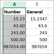
Works very much like the General format but varies how it shows numbers with decimal place separators and negative numbers. Here are some examples of how both formats display numbers:
|
|
Currency |
Shows a monetary symbol with numbers. You can specify the number of decimal places with Increase Decimal or Decrease Decimal.
|
|
Accounting |
Also used for monetary values, but aligns the currency symbols and decimal points of numbers in a column. |
|
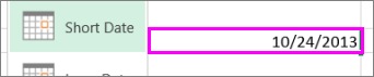
Short Date |
Shows date in this format:
|
|
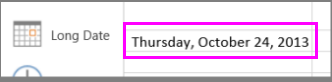
Long Date |
Shows month, day and year in this format:
|
|
Time |
Shows number date and time serial numbers as time values. |
|
Percentage |
Multiplies the cell value by 100 and displays the result with a percent (%) symbol. Use Increase Decimal or Decrease Decimal to specify the number of decimal places you want.
|
|
Fraction |
Shows the number as a fraction. For example, 0.5 displays as ½. |
|
Scientific |
Displays numbers in exponential notation, replacing part of the number with E+n, where E (Exponent) multiplies the preceding number by 10 to the nth power. For example, a 2-decimal Scientific format displays 12345678901 as 1.23E+10, which is 1.23 times 10 to the 10th power. To specify the number of decimal places you want to use, apply Increase Decimal or Decrease Decimal. |
|
Text |
Treats the cell value as text and displays it exactly as you type it, even when you type numbers. Learn more about formatting numbers as text. |
Transcript
What is a number format?
Number formats are used to control the display of cell values that contain numeric data. This numeric data can include things like dates, times, costs, percentages, and anything else expressed as a number. The most important thing to understand about number formats is that they only affect how a number looks—they have no effect on the actual value stored by Excel.
Let’s take a look.
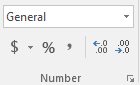
The most common number formats are available on the home tab of the ribbon, in the Number format area. Here you’ll find formats for currency, numbers, date, time, and more.
To apply a number format, just select one or more cells and choose a format. Number formats only affect numbers; they have no effect on text.
Let’s format the rest of the values in our table.
After we have applied the formats, notice that Excel will display the name of the format when a cell is selected.
When you have multiple cells selected, you’ll see the format of the active cell displayed. Be aware that the active cell in a selection can vary, depending on how you select cells.
Most number formats have one or more options. To set number format options, and to see all number formats, visit the Format Cells dialog box. You can access this dialog by clicking the small arrow in the Number group on the ribbon or using the keyboard shortcut Ctrl-1. On the Number tab, you’ll find all the options available for each number format.
Let’s use the Format Cells dialog box to adjust the Fraction format. To get our fraction to display correctly, let’s format it to use hundredths.
Finally, remember that number formats only affect the display of a cell value, not the value itself. If we check the cells in our table, watching the formula bar, we see that the values are unchanged.
The value for Percentage looks different, but if we switch the format back to General, we see that the value being stored is, indeed, .05.
Number Formatting in Excel: Step-by-Step Tutorial (2023)
We all know how to apply the basic numeric and text formats to cells in Excel.
But do you know how you can add a desired number of decimals, scientific notations, currency symbols, and similar formats in Excel with only a click?
No? This article is for you. It delves into the details of number formatting in Excel. 🤩
Keep reading till the end, and download our free sample workbook here before you scroll down.
What are number formats?
Type something into a cell. What is its format?

By default, all cells of Excel will have the General format applied.
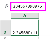
However, type in a big number that exceeds the size of the cell, and Excel would give you back something like 1.2E+12.

What is this? A scientific notation. Under General format, Excel replaces a number too big to fit the cell with its scientific notation.
To turn it into a number, change the format to ‘Numbers’ and adjust the cell size.

Check the formula bar to note how the number remains the same under both formats i.e. 1200000000000.
What changes is only the visual representation of the said number in Excel (decimal places added).
That is how formats work in Excel.
And you can change the format of a number with a mere click. Excel offers many number formats with useful variations to them.
Thousands separator
In the image below we have different numbers.

By now, it only seems like a number that is hard to read. Maybe that’s because it doesn’t yet have 1000s separators (any commas) to it.
- Select the cell.
- Go to Home > Number

- From the menu, go to More Number Formats

This launches the Format Cells dialog box.
You may use the keyboard shortcut (Control Key + 1) to launch the Format Cells dialog box.

- Go to Number Format.
- Check the ‘Use 1000 Separator’ box.

- Here are the results.

A shortcut to add the 1000s separator: Go to Home > Number > click on the comma symbol

However, this changes the number format to the Accounting format.

Controlling decimals
In the same example, as above, there are two decimals to the number.

But you want four decimal places to this number. How can this be done?
- Select the cell.
- Go to Home > Number > More Number Formats

- From the Format Cells dialog box, go to Number Format.
- Adjust the decimal places to four.

- Here are the results.

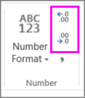
A shortcut to adjust decimal places. Go to Home > Number > Add decimals button

With every click, Excel adds another decimal position to the number.
The button with a right-headed arrow reduces a decimal position.
The button with a left-headed arrow adds a decimal position.
Show as percentage
Here is a decimal number that we want to be converted into a percentage.

To do this:
- Select the cell.
- Go to Home > Number > More Number Formats

- From the Format Cells dialog box, go to Number Format.
- Click on Percentage.

- Adjust the decimal places as desired.

- Here are the results.

A shortcut to convert a number into a percentage. Go to Home > Number > Click the % symbol

Number formatting presets
Excel offers a wide variety of number formatting presets. (You must’ve had a slight idea of that by now.)
These range from currency to accounting to dates and whatnot.
Let’s look into each of these formats below.
General number format preset
The general number format of Excel is the default format of any value in Excel.
All values in all cells of Excel will have the general number format by default.
- To apply the general format to any cell in Excel, select that cell.
- Press the Control key + 1 to launch the Format cells dialog box. That’s a handy shortcut 😊.
- Choose the ‘General number’ format.

- Values formatted as general numbers are displayed just the way they are.
Pro Tip!
Under the General number format, if the cell is not wide enough to contain a number, Excel would:
- Round a number with decimals to lesser decimal places; or
- Use scientific notation to express the number; or
- If the cell is too small to fit in the scientific notation for the number even, display a series of hashes only.
Number format preset
The Excel number format is used for simple numeric values
To apply the number format to any cell:
- Select the cell.
- Go to Home > Numbers > Drop Down Menu and click on Number Format.

The number format allows users three further variations to the final value:
- The decimal places. You can adjust decimal places to any desired number.

- The 1000 Separator. Check the box if you need 1000s separators to the value.

- The format of negative numbers. This could be in two colors (black or red) and enclosed within brackets or with a minus sign.

The Sample box gives a preview of what the final value may look like.

Must Note:
Under the Numbers format, if you type a number in a cell that is too big to fit in the cell, Excel might return a series of hashes only.

In such a case, one must know that the problem simply lies within the size of the cell. (that is too small to fit in the cell value).
To work this out, increase the width of the column until it is wide enough to fit in the cell value.

Currency format preset
The Currency format is used to denote currencies.
To format a number as currency:
- Go to Home > Numbers > Drop Down Menu > Click on Currency.

It allows you to adjust three options to your desire:
- The decimal places.

- The currency symbol.

- The format of negative numbers. This could be in two colors (black or red) and enclosed within brackets or with a minus sign.

Here is what a currency formatted number looks like.

Date format presets
There are two date formats offered by Excel – short date and long date.

To format a number as a date, go to Format Cells and choose the date format you’d want to be applied.

Excel offers a wide variety of formats for dates and days.
Here is how the date format works.

Pro Tip!
Type any number into Excel and apply the date formatting to it. Excel turns it into a date.
This is because Excel recognizes each date as a number. Where 1 is equal to 01 Jan 1900, 2 is equal to 02 Jan 1900, and so on.
Accounting format preset
Next is the accounting format preset.
This format is relevant when you’re working with financial data. For example, while preparing financial statements, forecasts, or similar reports.
To apply accounting format to a number:
- Go to Home > Numbers > Drop Down Menu > Click on Accounting Format.

It allows you to adjust two features to your desire:
- The decimal places.

- The currency symbol.

Here is what an accounting formatted number looks like.

Under the accounting format, 1000s separators and currency symbols are added by default. And negative numbers are enclosed in parenthesis i.e. $ (1925.60) etc.
Time format preset
Excel also offers a wide variety of ways how you may represent times in Excel.
To apply the time format, go to Format Cells and choose the time format you’d want to apply.

You can format it to be displayed as HH:MM:SS or any other way you like.
Here is how the time format looks in action.

Formatting shortcuts
There are plenty of shortcuts on how you may quickly format cell values in Excel.
You can format numbers by using these keyboard shortcuts. Simply select the cell (or cells) where you want the formatting applied and use the shortcuts below.
- Control Key + Shift Key + ~ : Applies the General format
- Control Key + Shift Key + ! : Applies the Number format
- Control Key + Shift Key + $ : Applies the Currency format
- Control Key + Shift Key + % : Applies the Percentage format
- Control Key + Shift Key + ^ : Applies the Scientific notation format
- Control Key + Shift Key + # : Applies the Date format
- Control Key + Shift Key + @ : Applies the Time format
All of these are shortcut keys and only apply the default formats (like the default two decimal places or HH:MM:SS AM/PM format etc.)
Custom formatting
Tired already? However, the number formats list has yet not come to an end.
The last and the most important number format of Excel is the Custom Format.
Under this format, you can customize a number format as needed.
- Go to Home > Numbers > Drop Down Menu > More Number Formats.
- Click on Custom Format.

- Under the custom formatting, you see different formats.

- To create a custom number format, choose the format that closely matches what you are looking for.
- Customize it as needed (keep an eye on the sample to see if you’ve reached your desired format).
- And save your custom number format.
That’s it – Now what?
Like all the amazing tools offered by Microsoft Excel, number formats are a whole toolkit in itself.
There’s so much to explore, and this article only gives you an idea of how you can come up with different visual representations of the same value.
Not only that, but if you fail to find the format you’re looking for – you can customize one for yourself. That’s where the possibilities become limitless.
Want to learn further? Learn the core functions of Excel including the VLOOKUP, SUMIF, and IF functions.
You need not go any further to master these functions. Click here to sign up for my free 30-minute email course that will take you through these and many more functions in no time.
Kasper Langmann2023-01-19T12:13:39+00:00
Page load link
If you used Excel in any shape or form, there is a pretty good chance that you’ve used the formatting and number formatting features. Formatting options like number, currency, percentage, date and time values are easily accessible to users. However, that’s not all there is in the world of text and number formatting. Going down the rabbit hole, custom formatting can help you fully configure Excel’s built-in settings for formatting.
The main advantage of this approach is that you can alter the look of your data without changing the actual values. This means that you do not need to use additional spaces or formulas to create the layout you want and preserve the raw data.
If you want to modify your data anyways, or need to change a value inside a formula, you can use the TEXT function with all custom formatting syntax we are going to cover in this article. It should be noted that the TEXT function returns a text, and the return value cannot be used in mathematical calculations. If you do, you will receive a #VALUE! error. In this article we’re going to be using a workbook template. You can download it below.
How to create a custom number format in Excel
- Select the cell to be formatted and press Ctrl+1 to open the Format Cells dialog. An alternative way to do is by right-clicking the cell and then going to Format Cells > Number Tab.
- Under Category, select Custom.
- Type in the format code into the Type
- Click OK to save your changes.
Note: In Format Cells dialog you can modify the built-in format codes by selecting the format you want to modify in its own category (i.e. Currency > ($1,234.10)) and then selecting Custom Category. Don’t worry, Excel will not let you delete built-in formats.

Basics
Syntax
The format code has 4 sections separated by semicolons.
POSITIVE; NEGATIVE; ZERO; TEXT
These sections are optional,
- If a code contains only 1 section, the format is applied to all number types — positive, negative and zero.
- If a code contains 2 sections, the first section is used for positive and zero values, while the second section is applied to negative values.
- If a code contains 3 sections, the first is for positive, the second is for negative, and the third is for zero.
- A code only affects text values if all sections exist.
Default format type in Excel is called General. You can type General for sections you don’t want formatted. Make sure you use a minus sign (-) with General if you want to skip negative values.
If you want to completely hide a type, leave it blank after the semicolon. For example; to hide 0 values, General;-General;;General
Placeholders and the Cheat Sheet
| Placeholder | Description | Raw Value | Format Code | Formatted Value |
| General | Default format | 1234.567 | General | 1234.567 |
| # | Placeholder for digits (numbers) and does not add any leading zeroes. | 1234.567 | #####.#### | 1234.567 |
| 0 | Placeholder for digits (numbers) and add any leading zeroes. | 1234.567 | 00000.0000 | 01234.5670 |
| ? | Placeholder for digits (numbers) and add space characters. | 1234.567 | ?????.???? | 1234.567 |
| . | Placeholder for the decimal place. | 1234.567 | 0.00 | 1234.57 |
| _ | Adds a blank space, to the width of the following character. You can use in combination with parentheses to add left and right indents, _( and _) respectively. | 99 | _(#_);(#) | 99 |
| -25 | (25) | |||
| 58 | 58 | |||
| 12 | 12 | |||
| -71 | (71) | |||
| 36 | 36 | |||
| * | Repeats the character after asterisk until the width of the cell is filled. | 66 | 0 *! | 66 !!!!!!!!!!!!!!! |
| Full Name | @ *_ | Full Name ____ | ||
| % | Convert value to a percentage with % sign | 0.12 | % | 12% |
| , | Thousands separator | 1234.567 | #, | 1 |
| 12345678 | #, | 12,346 | ||
| 12345678 | #,###, | 12,346 | ||
| 12345678 | #,, | 12 | ||
| E | Scientific notation format. Requires a ‘+’ symbol after, and a digit placeholder before and after. | 1234.567 | 0.00E+00 | 1.23E+03 |
| / | Represents fractions | 1.234 | # ##/## | 1 11/47 |
| 1.234 | # 000/000 | 1 117/500 | ||
| 1.234 | ##/## | 58/47 | ||
| «» | Text placeholder for multiple characters | 1234.567 | #,##0 «km/h» | 1,235 km/h |
| Good | «Result is: «@ | Result is: Good | ||
| Text placeholder for single character | 1234 | #.00, K | 1.23 K | |
| 1234567 | #.00,, M | 1.23 M | ||
| @ | Placeholder for text | Bad | «Result is: «@ | Result is: Bad |
| [color] | Change Color of value. Options: [Black], [Green], [White], [Blue], [Magenta], [Yellow], [Cyan], [Red] | 1234.567 | [Green]#,##0.00_); [Red](#,##0.00); [Blue]0.00_); [Magenta]@ |
1,234.57 |
| -1234.567 | (1,234.57) | |||
| 0 | 0.00 | |||
| This is a text | This is a text |
Common Practices
Display and control of the first digit and decimals
Decimal places in the code are indicated with a period (.). Number of zeroes after the period (.) define the number of decimal places. For example,
- 0 — display 1 decimal place
- 00 — display 2 decimal places
If the number has more decimals than the decimal placeholders defined, the number will be rounded to the nearest number of placeholders.
| Raw Value | Format Code | Formatted Value |
| 123.4 | 0.0 | 123.4 |
| 123.4 | 0.00 | 123.40 |
| 123.45 | 0.00 | 123.45 |
| 123.45 | 0.00 | 123.46 |
| 123.456 | 0.0 | 123.5 |
Alternatively, hash (#) and question mark (?) symbols can be used as decimal places. However, because any missing decimal places will be filled with zeroes, using zeroes instead will be easier to read.
| Raw Value | Format Code | Formatted Value |
| 0.25 | 0.00 | 0.25 |
| 0.25 | #.## | .25 |
| 123 | 0.00 | 123.0 |
| 123 | #.?? | 123.00 |
| 123 | #.## | 123. |
Add text to numbers
Custom text can be added to the beginning or the end of a value. Text and characters should be added inside quotes («») and backslashes (). You can use backslash () to add single character.
| Raw Value | Format Code | Formatted Value |
| 123.4 | 0.0 «ft.» | 123.4 ft. |
| 123.4 | 0.00 l | 123.40 l |
| 123.45 | «Approx.» 0 | Approx. 123 |
| 123.45 | «Result:» 0.00 C | Result: 123.46 C |
| Bad | «Result is: «@ | Result is: Bad |
Quotation marks or backslashes are not necessary for spaces ( ) and some special characters.
| Symbol | Description |
| + and — | Plus and minus signs |
| ( ) | Left and right parenthesis |
| : | Colon |
| ^ | Caret |
| ‘ | Apostrophe |
| { } | Curly brackets |
| < > | Less-than and greater than signs |
| = | Equal sign |
| / | Forward slash |
| ! | Exclamation point |
| & | Ampersand |
| ~ | Tilde |
| Space character |
Below are some special characters you can use by copying or typing in the numerical code while pressing down Alt button.
| Symbol | Code | Description |
| ™ | Alt+0153 | Trademark |
| © | Alt+0169 | Copyright symbol |
| ° | Alt+0176 | Degree symbol |
| ± | Alt+0177 | Plus-Minus sign |
| µ | Alt+0181 | Micro sign |
Hide value
If you leave any number of sections blank, the value of those sections will be hidden. A section should always be separated (defined) by a semicolon (;). Here are some examples,
| Raw Value | Format Code | Formatted Value |
| 1 | 0;;0; | 1 |
| -2 | 0;;0; | |
| 0 | 0;;0; | 0 |
| Some text | 0;;0; | |
| 1 | ;(0);;@ | |
| -2 | ;(0);;@ | (2) |
| 0 | ;(0);;@ | |
| Some text | ;(0);;@ | Some Text |
| 1 | ;;; | |
| -2 | ;;; | |
| 0 | ;;; | |
| Some text | ;;; |
Replace zeroes with dashes
Zeroes can make data tables look more complicated than they actually are. You can hide them completely by using the previous method, or replace them with any character of your choice. Dash (-) is a common example. All you need to is place a dash into the ‘Zero section’.
| Raw Value | Format Code | Formatted Value |
| 0 | General;-General;»-«;General | — |
| 3487 | General;-General;»-«;»-« | — |
| 12 | #,##0.00;(#,##0.00);»-«; | — |
Start with zeroes
If try to enter a ZIP number that starts with 0, the leading zeroes will be removed automatically by Excel. To keep the leading zeros, use zero (0) placeholder for whole numbers.
| Raw Value | Format Code | Formatted Value |
| 10010 | 00000 | 10010 |
| 3487 | 00000 | 03487 |
| 12 | 00000 | 00012 |
| 0 | 00000 | 00000 |
| 123456 | 00000 | 123456 |
Dealing with thousands, millions, and more
You may have noticed that ‘0.0’ or other simple formats do not separate thousands or millions. Adding a comma into the code will insert commas to separate numbers.
| Raw Value | Format Code | Formatted Value |
| 1234 | #,##0 | 1,234 |
| 123456 | #,##0 | 123,456 |
| 12345678 | #,##0 | 12,345,678 |
| 123456.789 | #,##0 | 123,457 |
| 123456.789 | #,##0.0 | 123,456.8 |
There must be placeholders for numbers smaller than one thousand, otherwise such values will be hidden. This behavior allows us to round and format our value to show only thousands or millions.
| Raw Value | Format Code | Formatted Value |
| 1234 | #, | 1 |
| 123456 | #, | 123 |
| 12345678 | #, | 12345 |
| 12345678 | #,, | 12 |
| 123456 | #.0, K | 123.5 K |
| 12345678 | #.0,, M | 12.3 M |
Display numbers as phone numbers
Phone numbers can be hard to read without any separators. Custom Number Format Codes is perfect for this job. The hash (#) character should be your best bet to avoid any redundancy of placeholders (0, ?)
| Raw Value | Format Code | Formatted Value |
| 1234567890 | (###) ###-#### | (123) 456-7890 |
| 12345678900 | (###) #### #### | (123) 4567 8900 |
| 1234567890 | (##) #### #### | (12) 3456 7890 |
Showing Month and Weekday Names
Date and time values are stored as numbers in Excel. When you enter a date, Excel automatically converts it into a numerical value, and then formats the cell.
Before jumping into the code, let’s review some basics. Formatting code has special placeholders for date and time formatting that behave a bit differently. For example, while m and mm will show month as a number, mmm and mmmm will show as a text string. Below are some examples.
| Raw Value | Format Code | Formatted Value |
| 4/1/2018 | m | 4 |
| 4/1/2018 | mm | 04 |
| 4/1/2018 | mmm | Apr |
| 4/1/2018 | mmmm | April |
| 4/1/2018 | mmmmm | A |
| 4/1/2018 | d | 1 |
| 4/1/2018 | dd | 01 |
| 4/1/2018 | ddd | Sun |
| 4/1/2018 | dddd | Sunday |
| 4/1/2018 11:59:31 PM | dddd, mmmm dd, yyyy h:mm AM/PM;@ | Sunday, April 01, 2018 11:59 PM |
Here is the full list of options for the date 4/1/2018 23:59:31 ,
| Format Code | Description | Example (4/1/2018 23:59:31) |
| yyyy | Displays the year as a four-digit number. | 2018 |
| yy | Displays the year as a two-digit number. | 18 |
| m | Displays the month as a number without a leading zero. | 4 |
| mm | Displays the month with a leading zero. | 04 |
| mmm | Displays the month as text, as an abbreviation. | Apr |
| mmmm | Displays the month as text. | April |
| mmmmm | Displays the month as a single character | A |
| d | Displays the day as a number, without a leading zero. | 1 |
| dd | Displays the day as a number, with a leading zero. | 01 |
| ddd | Displays the day as a day of the week, as an abbreviation. | Sun |
| dddd | Displays the day as a day of the week, without abbreviation | Sunday |
| h | Displays the hour without a leading zero. | 23 |
| hh | Displays the hour with a leading zero. | 23 |
| [h] | Displays elapsed time in hours (to be used when the time value exceeds 24 hours). | 1036607 |
| m | Displays the minute without a leading zero. | 4 |
| mm | Displays the minute with a leading zero. | 04 |
| [m] | Displays elapsed time in minutes (to be used when the time value exceeds 60 minutes). | 62196479 |
| s | Displays the second without a leading zero. | 31 |
| ss | with a leading zero. | 31 |
| [s] | Displays elapsed time in seconds (to be used when the time value exceeds 60 seconds). | 3731788771 |
| AM/PM | Converts to 12-hour time. Displays either AM/am/A/a or PM/pm/P/p depending on the time of day. | PM |
| am/pm | pm | |
| A/P | P | |
| a/p | p |
Come in Colors Everywhere
Number Formatting can be used color sections of a code. A common example is using the color red for negative numbers. Color code must be placed inside square brackets (i.e. [color]), and entered at the beginning of a section. Here are some available colors,
- [Black]
- [Blue]
- [Cyan]
- [Green]
- [Magenta]
- [Red]
- [White]
- [Yellow]
| Raw Value | Format Code | Formatted Value |
| 1234.567 | [Green]#,##0.00_);[Red](#,##0.00);[Blue]0.00);[Magenta]@ | 1,234.57 |
| -1234.567 | (1,234.57) | |
| 0 | 0.00 | |
| This is a text | This is a text |
Conditions
Although Excel has conditional formatting menu, basic conditions can be applied through code. Condition should be placed inside square brackets (i.e. [condition]) just like colors. Conditions are similar to the conditions in some functions (i.e. SUMIF). First add a logical operator, and then a value. For example, “[>=1000000]” means “if value of cell is greater than or equal to 1,000,000 apply the following format”. Conditions should come before the actual code, again, just like with colors. If you want to a color as well, the color code should come first.
Another important thing to note here is, that section structure changes from Positive, Negative, Zero, Text to First Condition, Second Condition (if exists), if previous conditions are not applied. There should be at least two sections for conditions.
If you enter only one condition code and then save the format, Excel will automatically add the second section with «;General». This means that if the condition is not met, General format will be used.
| Raw Value | Format Code | Formatted Value |
| 1234567890 | [>=1000000]#,##0,,»M»;[>=1000]#,##0,»K»;0 | 1,235M |
| 12345 | 12K | |
| 1 | [=1]0″ apple»;0″ apples» | 1 apple |
| 10 | 10 apples | |
| 25 | [Green][>=85]»PASSED»;[Blue][>=60]»RE-CHECK»;[Red]»FAILED» | FAILED |
| 72 | RE-CHECK | |
| 91 | PASSED |
Excel Number Formats
Number Formats
The default Number format is General.
Why change number formats?
- Make data explainable
- Prepare data for functions, so that Excel understands what kind of data you are working with.
Examples of number formats:
- General
- Number
- Currency
- Time
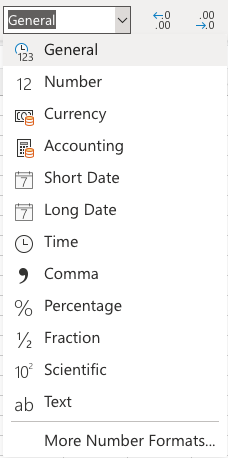
Number formats can be changed by clicking the Number format dropdown, accessed in the Ribbon, found in the Numbers group.
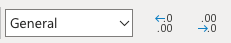
Note: You can switch the Ribbon view to access more Number format options.
Example
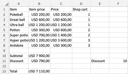
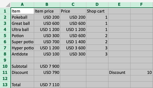
In the example we have cells that represent prices, which can be formatted as Currency.
Let’s try to change the format of the prices to the Currency Number format.
Step by step:
- Mark the range
B2:C8 - Click the Number format dropdown menu
- Click the Currency format
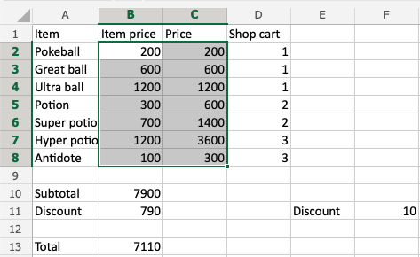
That’s it! The Number format was changed from General to Currency.
Note: It will use your local currency by default.
Now, do the same for B10, B11 and B13:
Did you make it?
Note: The currency can be changed. For example instead of using USD like in the example you can decide for $ or EUR. It is changed in the dropdrop menu, clicking the More Number Formats in the bottom of the menu. Then, clicking on Currency.
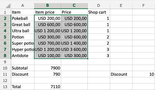
Notice that the numbers look like a mess. Let’s solve that by decreasing the decimals. This helps to make the presentation more neat.
Decimals
The number of decimals can be increased and decreased.
There are two commands:
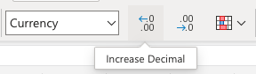
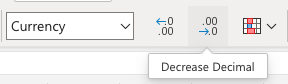
- Increase Decimal
- Decrease Decimal
Clicking them reduces or increases the number of decimals.
The commands can be found next to the Number format dropdown menu.
Note: Decreasing Decimals can make Excel round up or down numbers as more decimals get removed. This may be confusing if you are working on advanced calculations which require accurate numbers.
Let’s clean this up, step by step:
- Mark the range
B2:C8 - Click the Decrease Decimal button two times
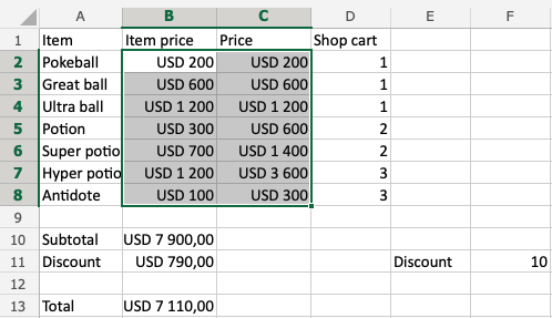
Great!
Do the same for B10, B11 and B13:
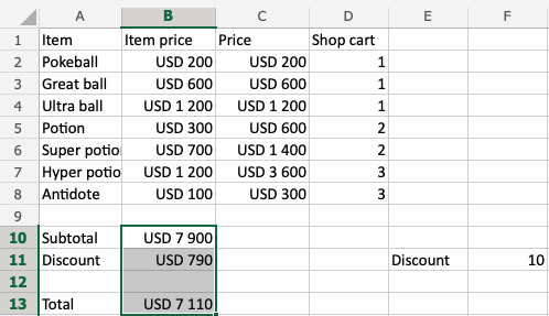
That looks a lot better!
Pro tip: The arrow in the angle in the top left corner by
row 1 and column A can be clicked to mark all cells in the sheet. This can be useful if you want to change the Number format or change Decimals for all cells.
Chapter summary
Number formats can be changed to make the spreadsheet more understandable or to prepare cells for functions. You can increase and decrease decimals to make the presentation neat.
Lesson 8: Understanding Number Formats
/en/excelformulas/doublecheck-your-formulas/content/
What are number formats?
Whenever you’re working with a spreadsheet, it’s a good idea to use appropriate number formats for your data. Number formats tell your spreadsheet exactly what type of data you’re using, such as percentages (%), currency ($), times, dates, and so on.
Watch the video below to learn more about number formats in Excel.
Why use number formats?
Number formats don’t just make your spreadsheet easier to read—they also make it easier to use. When you apply a number format, you’re telling your spreadsheet exactly what kinds of values are stored in a cell. For example, the date format tells the spreadsheet that you’re entering specific calendar dates. This allows the spreadsheet to better understand your data, which can help ensure that your data remains consistent and that your formulas are calculated correctly.
If you don’t need to use a specific number format, the spreadsheet will usually apply the general number format by default. However, the general format may apply some small formatting changes to your data.
Applying number formats
Just like other types of formatting, such as changing the font color, you’ll apply number formats by selecting cells and then choosing the desired formatting option. Every spreadsheet program allows you to add number formatting, but the process will vary depending on which application you’re using:
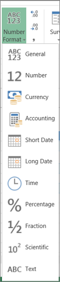
- For Microsoft Excel 2007-2019, go to the Home tab, click the Number Format drop-down menu in the Number group, and select the desired format. You can also click one of the quick number-formatting commands below the drop-down menu.

- For Excel 2003 and earlier, go to Format > Cells.
- For Google Sheets, click the More Formats button near the left side of the toolbar—this button will look like the numbers 123. To the left of the command, you can also click the Currency or Percent commands to quickly apply those formats.
For most versions of Microsoft Excel, you can also select the desired cells and press Ctrl+1 on your keyboard to access more number-formatting options.
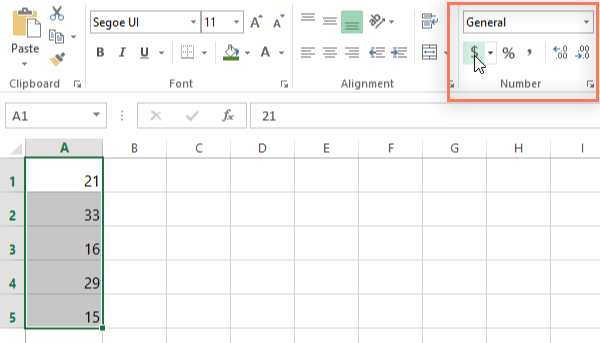
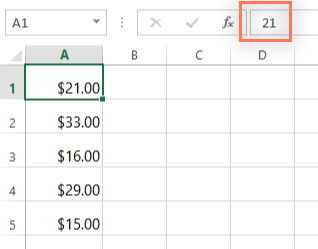
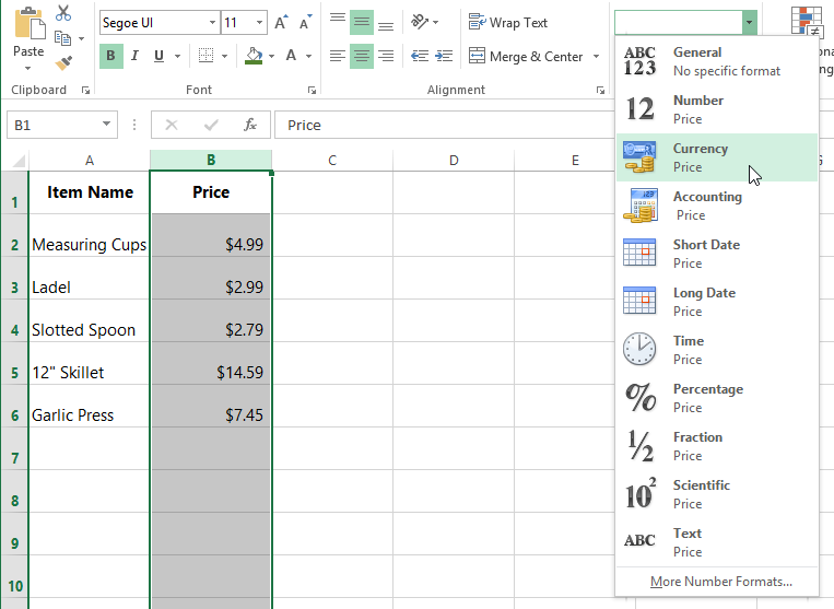
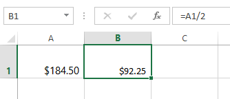
In this example, we’ve applied the Currency number format, which adds currency symbols ($) and displays two decimal places for any numerical values.
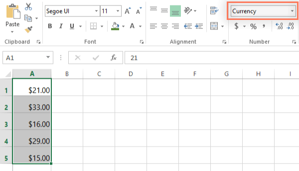
If you select any cells with number formatting, you can see the actual value of the cell in the formula bar. The spreadsheet will use this value for formulas and other calculations.
Using number formats correctly
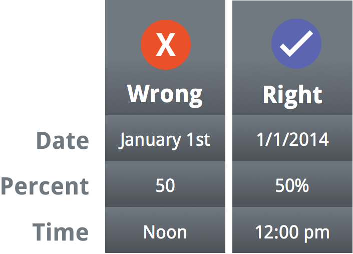
There’s more to number formatting than selecting cells and applying a format. Spreadsheets can actually apply a lot of number formatting automatically based on the way you enter data. This means you’ll need to enter data in a way the program can understand, and then ensure that those cells are using the proper number format. For example, the image below shows how to use number formats correctly for dates, percentages, and times:
Now that you know more about how number formats work, we’ll look at a few different number formats in action.
Percentage formats
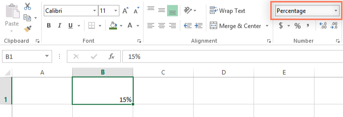
One of the most helpful number formats is the percentage (%) format. It displays values as percentages, such as 20% or 55%. This is especially helpful when calculating things like the cost of sales tax or a tip. When you type a percent sign (%) after a number, the percentage number format will be be applied to that cell automatically.
As you may remember from math class, a percentage can also be written as a decimal. So 15% is the same thing as 0.15, 7.5% is 0.075, 20% is 0.20, 55% is 0.55, and so on. You can review this lesson from our Math tutorial to learn more about converting percentages to decimals.
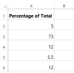
There are many times when percentage formatting will be useful. For example, in the images below, notice how the sales tax rate is formatted differently for each spreadsheet (5, 5%, and 0.05):
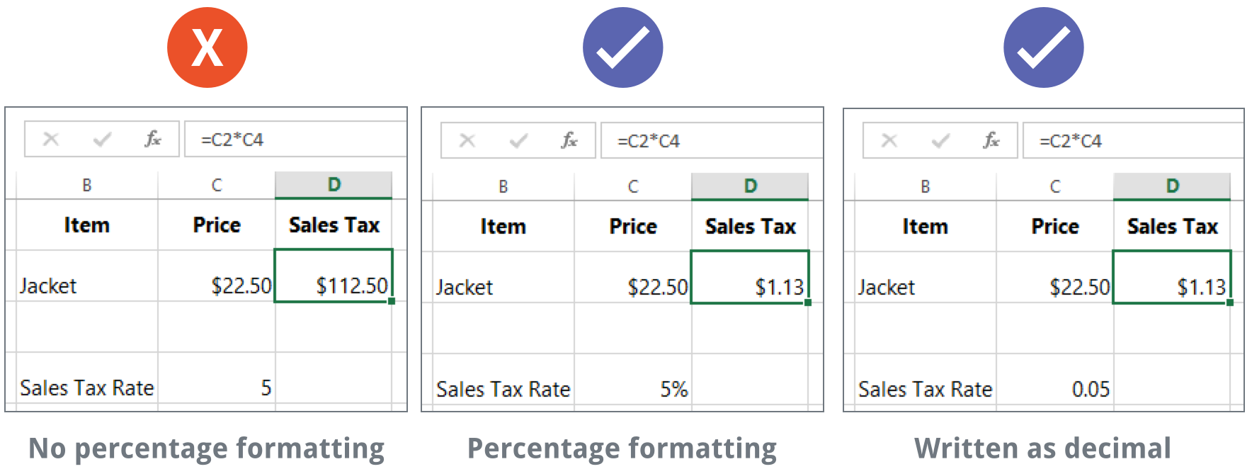
As you can see, the calculation in the spreadsheet on the left didn’t work correctly. Without the percentage number format, our spreadsheet thinks we want to multiply $22.50 by 5, not 5%. And while the spreadsheet on the right still works without percentage formatting, the spreadsheet in the middle is easier to read.
Date formats
Whenever you’re working with dates, you’ll want to use a date format to tell the spreadsheet that you’re referring to specific calendar dates, such as July 15, 2014. Date formats also allow you to work with a powerful set of date functions that use time and date information to calculate an answer.
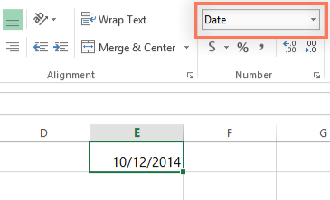
Spreadsheets don’t understand information the same way a person would. For instance, if you type October into a cell, the spreadsheet won’t know you’re entering a date so it will treat it like any other text. Instead, when you enter a date, you’ll need to use a specific format your spreadsheet understands, such as month/day/year (or day/month/year depending on which country you’re in). In the example below, we’ll type 10/12/2014 for October 12, 2014. Our spreadsheet will then automatically apply the date number format for the cell.
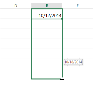
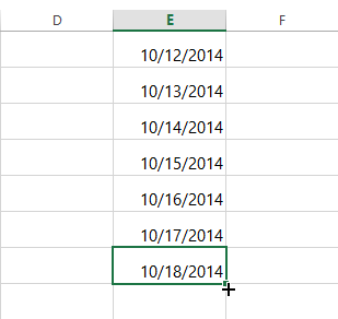
Now that we have our date correctly formatted, we can do lots of different things with this data. For example, we could use the fill handle to continue the dates through the column, so a different day appears in each cell:
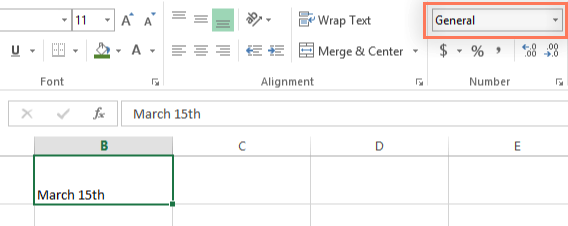
If the date formatting isn’t applied automatically, it means the spreadsheet did not understand the data you entered. In the example below, we’ve typed March 15th. The spreadsheet did not understand that we were referring to a date, so this cell is still using the general number format.
On the other hand, if we type March 15 (without the «th»), the spreadsheet will recognize it as a date. Since it doesn’t include a year, the spreadsheet will automatically add the current year so the date will have all of the necessary information. We could also type the date several other ways, such as 3/15, 3/15/2014, or March 15 2014, and the spreadsheet would still recognize it as a date.
Try entering the dates below into a spreadsheet and see if the date format is applied automatically:
- 10/12
- October
- October 12
- October 2014
- 10/12/2014
- October 12, 2014
- 2014
- October 12th
If you want to add the current date to a cell, you can use the Ctrl+; shortcut, as shown in the video below.
Other date formatting options
Some programs have more date formatting options, which can change the way dates appear in your spreadsheet. Again, this process this may vary slightly based on the spreadsheet program you’re using. To access these options in Excel 2007-2019, select the Number Format drop-down menu and choose More Number Formats.
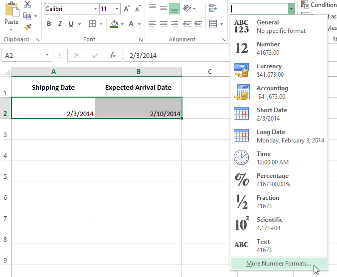
A dialog box will appear. From here, you can choose the desired date formatting option.
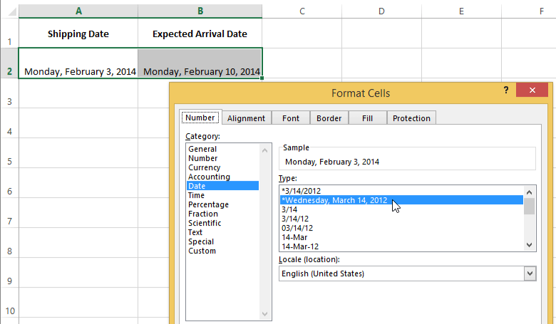
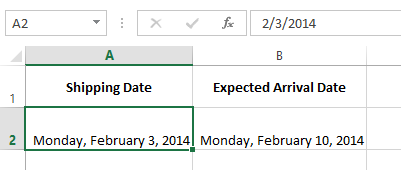
As you can see in the formula bar, a custom date format doesn’t change the actual date in our cell—it just changes the way it’s displayed.
Number formatting tips
Here are a few tips for getting the best results with number formatting:
- Apply number formatting to an entire column: If you’re planning to use one column for a certain type of data, like dates or percentages, you may find it easiest to select the entire column by clicking the column letter and then applying the desired number formatting. This way, any data you add to this column in the future will already have the correct number format. Note that the header row usually won’t be affected by number formatting.

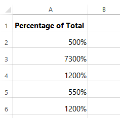
- Double-check your values after applying number formatting: If you apply number formatting to existing data, you may have unexpected results. For example, applying percentage (%) formatting to a cell with a value of 5 will give you 500%, not 5%. In this case, you’d need to retype the values correctly in each cell.


- If you reference a cell with number formatting in a formula, the spreadsheet may automatically apply the same number formatting to the new cell. For example, if you use a value with currency formatting in a formula, the calculated value will also use the currency number format.

- If you want your data to appear exactly as entered, you’ll need to use the text number format. This format is especially good for numbers you don’t want to perform calculations with, such as phone numbers, zip codes, or numbers that begin with 0: for example, «02415». For best results, you may want to apply the text number format before entering data in those cells.
To learn more about applying number formatting in a specific spreadsheet application, review the appropriate lesson from our tutorials below:
- Excel 2007-2019
- Excel 2003
- Google Sheets
/en/excelformulas/practice-reading-formulas/content/