What is not a date function in excel

To get detailed information about a function, click its name in the first column.

Note: Version markers indicate the version of Excel a function was introduced. These functions aren’t available in earlier versions. For example, a version marker of 2013 indicates that this function is available in Excel 2013 and all later versions.

Function	Description
DATE function	Returns the serial number of a particular date
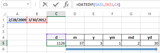
DATEDIF function	Calculates the number of days, months, or years between two dates. This function is useful in formulas where you need to calculate an age.
DATEVALUE function	Converts a date in the form of text to a serial number
DAY function	Converts a serial number to a day of the month
DAYS function	Returns the number of days between two dates
DAYS360 function	Calculates the number of days between two dates based on a 360-day year
EDATE function	Returns the serial number of the date that is the indicated number of months before or after the start date
EOMONTH function	Returns the serial number of the last day of the month before or after a specified number of months
HOUR function	Converts a serial number to an hour
ISOWEEKNUM function	Returns the number of the ISO week number of the year for a given date
MINUTE function	Converts a serial number to a minute
MONTH function	Converts a serial number to a month
NETWORKDAYS function	Returns the number of whole workdays between two dates
NETWORKDAYS.INTL function	Returns the number of whole workdays between two dates using parameters to indicate which and how many days are weekend days
NOW function	Returns the serial number of the current date and time
SECOND function	Converts a serial number to a second
TIME function	Returns the serial number of a particular time
TIMEVALUE function	Converts a time in the form of text to a serial number
TODAY function	Returns the serial number of today’s date
WEEKDAY function	Converts a serial number to a day of the week
WEEKNUM function	Converts a serial number to a number representing where the week falls numerically with a year
WORKDAY function	Returns the serial number of the date before or after a specified number of workdays
WORKDAY.INTL function	Returns the serial number of the date before or after a specified number of workdays using parameters to indicate which and how many days are weekend days
YEAR function	Converts a serial number to a year
YEARFRAC function	Returns the year fraction representing the number of whole days between start_date and end_date

Important: The calculated results of formulas and some Excel worksheet functions may differ slightly between a Windows PC using x86 or x86-64 architecture and a Windows RT PC using ARM architecture. Learn more about the differences.

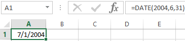
The DATE function is a financial analyst’s best pal and categorized as a Date/Time function in Excel. The criticality of the DATE function’s role is sourced from Excel’s reluctance to keep the day, month, and year as a date. Instead, Excel stores them as a serial number.

Directly handing over dates as a text string may not work well for all Excel functions. So, we will supply the dates as a serial number using the DATE function to ensure that Excel and our worksheet formulas understand the instructions properly.

Syntax

The syntax of Excel Date function is as follows:

=DATE(year, month, day)

Arguments:

year – This is a required argument that represents the year component in the date. Enter it as a 4 digit number; entering a single digit will result in Excel automatically adding 1900 to it.

For example, entering year as ’10’ will instruct the formula to interpret the year argument as ‘1910’.

Excel refers to your computer’s date system set up to interpret the Year argument. Note that entering a negative value or a value greater than 9999 will return a #NUM! error.

month – This is a required argument that represents the month component in the date. Ideally, it must be an integer from 1 to 12 (January to December).

Alternatively, if you input a number greater than 12, Excel will count that many months starting from January of the year specified in the year argument. For example, entering year as 2001 and month as 18 will return a serial number that represents June 01, 2002. Note that Excel will return the date as the first date of the interpreted month (June 01 in our case), regardless of what you input in the date argument.

On the other hand, if you enter a value less than 1, Excel will reduce that many months from January of the year specified, plus 1. For example, if you enter month as -10 and year as 2001, Excel will return a serial number that represents February 01, 2000.

day – This is a required argument that represents the day component of the date. While in an ideal case, you will enter an integer from 1 to 31 as the date argument, it can be supplied as any other positive or negative integer and Excel will apply the same principles to compute the date as it does for the month argument.

Important characteristics of the DATE function

• DATE function returns a #NUM! error when year argument is supplied with a negative number or a number greater than 9999.
• DATE function returns a #VALUE! error when any of its three arguments is supplied with a non-numeric value.
• If you see the Excel DATE function is returning a serial number like 36557 instead of a date, you will need to change the cell’s format. To do this, select the cell containing the returned date and search for the ‘Short Date’ option in the drop-down menu of cell formatting options in the ‘Number group’. These options sit on Excel’s Home Tab that appears at the top left.

Examples of the DATE function

Now let’s have a look at some of the examples of the DATE function in Excel.

Example 1 – The Plain – Vanilla DATE formula

In its purest form, this is what a DATE formula looks like:

=DATE(2001, 3, 15)

This formula returns a serial number that corresponds to the date March 15, 2001.

However, the formula can be slightly tweaked to incorporate the TODAY function encapsulated inside the YEAR function in Excel as well, like so:

=DATE(YEAR(TODAY()), 3, 15)

This formula will fetch the serial number for the current year (and the specified month and day), and return 03/15/2021.

Much the same way, you can use the TODAY function for the month argument as well, like so:

=DATE(YEAR(TODAY()), MONTH(TODAY()), 15)

This formula will fetch the serial number for the current year as well as the current month (and the specified day), and return 02/15/2021.

Example 2 – Using Cell References in DATE function Arguments

If the values you want to supply in the arguments are stored in cells on your spreadsheet, you can reference those cells, like so:

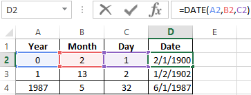
=DATE(A2, B2, C2)

With the values supplied from column A, the DATE function returns 04/30/2001.

Example 3 – Converting a number into a date using the DATE function

Let’s say you scalped the internet and landed on a large data set with dates written in a format that Excel does not understand (for example, 20052005).

In that (or similar) case, we can use the following formula to help Excel make sense of the data and interpret these numbers appropriately as dates:

=DATE(RIGHT(A2, 4), MID(A2, 3, 2), LEFT(A2, 2))

Recommended Reading:  Excel MID Function

Addition and Subtraction of Dates With DATE function

We discussed earlier how Excel store dates as serial numbers. There is of course a logical reason why Excel does this – it enables us to add or subtract a specified number of days from a given date.

To illustrate how this works, we plugged the following formula into our sheet:

=DATE(2001, 3, 15) + 20

When you add a +20 at the end of this DATE formula, Excel will return the date 20 days after 03/15/2001, which is 04/04/2001.

Alternatively, to subtract a certain number of days, all you need to do is use a minus sign, like so:

=DATE(2001, 3, 15) - 10

But, let’s say you want to compute the number of days between today and another date. In that case, we will subtract both dates, like so:

=TODAY() - DATE(2021, 2, 20)

The formula will return the number of days between today (whenever that may be) and March 15, 2001.

Changing DATE format With DATE function

So, you added some neat formulas to your Excel sheet and everything worked out fine. But, let’s say you want to use different separators for the days (for example, ‘/’ instead of ‘-‘), or you want to use the name of the month instead of a number (for example, January instead of 01).

We discussed earlier that Excel will refer to your computer’s date format and uses the same format for displaying dates in a worksheet.

To change this format, you do not need a formula. Instead, you need to tweak some settings.

Select the cell that contains the output from the DATE function. Right-click, and choose «Format Cells». You should see the following dialogue box:

Choose the format of your preference and click «OK».

Conditional Formatting with DATE function

Let’s say you have a large data set and you want to separate the data points occurring before and after a certain date.

To do this, we will use Excel’s conditional formatting rules and instruct Excel to shade these 2 cells with 2 separate colors so it becomes easy for us to discern.

We have our dates listed out in column A, and we want to shade the dates occurring before 12/31/2012 in green, and the ones occurring after in red.

To illustrate the entire process, we will use the following formula as a starting point:

=$A2 < DATE(2012, 12, 31)

Notice how this formula returns a Boolean value but does not shade any cells.

Let’s move a step further and apply a shade.

Select the range A2:A8 and navigate to the «Conditional Formatting» drop-down menu in the «Styles» group under the «Home» tab, and select «Manage Rules»:

On the «Conditional Formatting Rules Manager» click the «New Rule» button.

After clicking on the «New Rule» you will see a list of Rule Types. Scroll over to «Use a formula to determine which cells to format» and choosing it will reveal a formula box. In this box, plug in the formula we used to fetch Boolean values and select the desired formatting, like so:

Click «OK» and you should return to the Conditional Formatting Rules Manager dialog box.

To shade the dates occurring after 12/21/2012 red, we will add another rule following the same process. The only difference, obviously, will be in the formula. Instead of using a ‘<‘, we will use a ‘>=’, like so: =$A2>=DATE(2012,12,31)

This is what the Rules Manager box should look like at this point. Make sure that the «Applies to» box contains the appropriate range.

As your final step, click on «Apply» and watch your date list switch colors.

I hope the guide gives you a confidence boost the next time you use DATE formulas in your worksheet. Remember, practice is key. By the time you are done practicing, we will have another Excel function for you to explore.

Author: Oscar Cronquist Article last updated on June 07, 2022

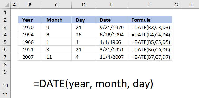
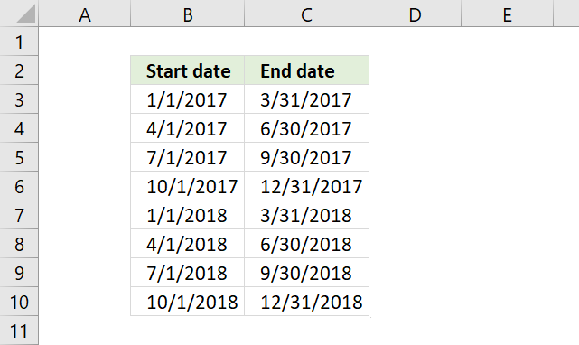
The DATE function returns a number that acts as a date in the Excel environment. The image above shows you the DATE function in column E. It uses three arguments, the first argument is the year found in column B.

The second argument is the month, shown in column C. Note that you need to use a number for the month.

The third argument is the day of the month, displayed in column D. Make sure you enter the correct day for the month, keep in mind most months have 30 days or 31 days. February has 28 days except for leap years that have 29 days.

1. Excel function syntax

DATE(year, month, day)

2. Arguments

year	A number equal or higher than 1900.
month	A number between 1 (January) and 12 (December). You can use larger numbers as well.
day	A number between 1 and 31 based on the number of days in the month specified in argument month.

Back to top

3. Add or subtract months and days

If you use a month number larger than 12, for example 13, DATE(2009,13,1) the DATE function returns 1/1/2010. Month number zero returns the previous month.

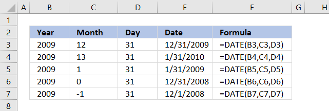
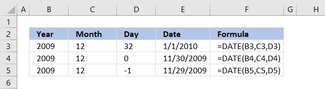
The same thing happens with a day number that is larger than 31 or smaller than 1.

You can use that to do dynamic date series or do date-based calculations.

Back to top

4. Date function example

The image above demonstrates the date function in column E, it uses values from column B, C and D.

Formula in cell F3:

=DATE(B3, C3, D3)

Back to top

5. What does the Date function do?

The DATE function returns an Excel date that you can use in formulas, Excel can’t calculate dates in formulas unless you reference a cell containing an Excel date or create an Excel date using the DATE function.

Hardcoding dates in a formula are not possible, use the DATE function to create an Excel date.

Why is that?
Excel uses numbers formatted as dates, 1 is 1/1/1900, and 1/1/2000 is 36526.

Prove it?
Sure, type 1 in a cell and press Enter. Select the cell and press CTRL + 1 to format the cell.

A dialog box appears, select Date in Category: and press the «OK» button.

Number 1 is now formatted as an Excel date, the cell shows 1/1/1900.

Back to top

6. Date function format

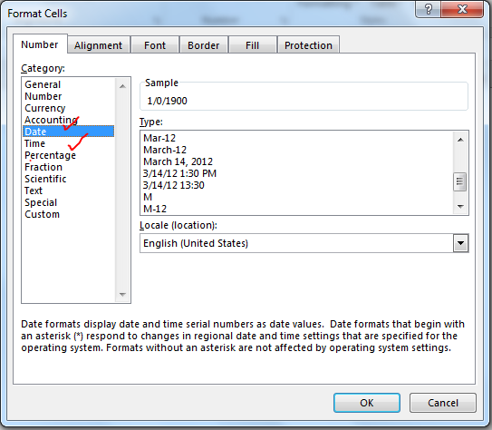
The animated image above shows you the «Format Cells» dialog box, it allows you to choose from many different date formatting types. Here is how:

1. Select the cell.
2. Press CTRL + 1 to open the «Format Cells» dialog box.
3. Select Date in the Category:, see the image above.
4. Pick a formatting type.
5. Press with left mouse button on «OK» button to apply changes.

You can also use the TEXT function to format dates.

Formula in cell B2:

=TEXT(DATE(1900, 1, 1), «d-m-yyyy»)

Back to top

Explaining formula in cell B2

Step 1 — Create an Excel date

The DATE function calculates a serial number that represents a specific date based on three arguments. Year, month, and day.

DATE(year, month, day)

DATE(1900, 1, 1)

returns 1.

Step 2 — Return a number formatted as a date

The TEXT function formats a cell value based on given placeholder characters.

TEXT(value, format_text)

TEXT(DATE(1900, 1, 1), «d-m-yyyy»)

becomes

TEXT(1, «d-m-yyyy»)

and returns 1-1-1900.

Back to top

7. Date function not working

1. Did you spell the DATE function correctly?
   
   Excel returns a #NAME? error if you didn’t.
2. Check the arguments, they must be numerical. Text is not allowed.
   
   Excel returns a #VALUE! error if any of the arguments contain a text value.
   year — a number equal or larger than 0 (zero)
   month — any number positive or negative
   day — any number positive or negative
3. Did you use exactly three arguments?
   
   Excel returns a dialog box: You’ve entered too many arguments for this function.
   DATE(year, month, day)
4. Excel Date function returns the wrong date.
   
   If you try a year before 1900 Excel returns a date that you probably didn’t expect. Here is how Excel came up with that date. 1900+1800 = 1/1/3700
5. The DATE function returns hashtags.
   
   The DATE function can’t return dates before 1/1/1900. The formula in cell B2 above tries to calculate an Excel date before 1/1/1900.

Back to top

8. How to make Excel order by date

The image above shows a list of dates in column B, here is how to sort the dates.

1. Press with right mouse button on any date in column B.
   A popup menu appears.
   
2. Press «Sort». Another popup menu appears.
3. Press either «Sort Oldest to Newest» or «Sort Newest to Oldest».

Here is how to sort the dates using a formula.

Formula in cell D2:

=LARGE($B$2:$B$17, ROWS($A$1:A1))

Back to top

Explaining formula in cell D2

Step 1 — Create a sequence of values from 1 to n

The ROWS function returns a number based on the number of rows in a cell reference.

ROWS(ref)

ROWS($A$1:A1)

returns 1.

Note that $A$1:A1 is a growing cell reference meaning it expands when you copy the cell and paste it to cells below.

Step 2 — Extract k-th largest serial number

The LARGE function calculates the k-th largest number.

LARGE(array, k)

LARGE($B$2:$B$17, ROWS($A$1:A1))

becomes

LARGE($B$2:$B$17, 1)

becomes

LARGE({45338; 53253; 49446; 51878; 48237; 52238; 44437; 53971; 49050; 47745; 45727; 45027; 49156; 49329; 48599; 49590}, 1)

and returns 53971 (10/6/2047) in cell D2.

Note, use the SMALL function if you want to sort the dates from oldest to newest.

Back to top

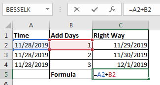
9. Date function add days

The formula in cell C3 adds 10/25/2024 with 10 days specified in cell B3.

Formula in cell C3:

=DATE(2024,10,25+B3)

Back to top

Explaining formula in cell C3

Step 1 — Add dates

The plus sign lets you add numbers in Excel formulas.

25+B3

becomes

25 + 10 equals 35.

Step 2 — Calculate serial number representing an Excel date

The DATE function calculates a serial number that represents a specific date based on three arguments. Year, month, and day.

DATE(year, month, day)

DATE(2024,10,25+B3)

becomes

DATE(2024,10,35)

and returns 45600 formatted as 11/4/2024 in cell C3.

Back to top

10. Date function subtract days

The formula in cell C3 subtracts 10/25/2024 with 10 days specified in cell B3.

Formula in cell C3:

=DATE(2024,10,25-B3)

Back to top

Explaining formula in cell C3

Step 1 — Subtract dates

The minus sign lets you subtract numbers in Excel formulas.

25-B3

becomes

25 — 10 equals 15.

Step 2 — Calculate serial number representing an Excel date

The DATE function calculates a serial number that represents a specific date based on three arguments. Year, month, and day.

DATE(year, month, day)

DATE(2024,10,25-B3)

becomes

DATE(2024,10,15)

and returns 45580 formatted as 11/4/2024 in cell C3.

Back to top

11. Date function add months

The formula in cell E3 adds months based on the number in cell B3 to a date specified in cell C3.

Formula in cell C3:

=DATE(YEAR(C3), MONTH(C3)+B3, DAY(C3))

Back to top

Explaining formula in cell C3

Step 1 — Calculate year

The YEAR function returns a number representing the year based on an Excel date (serial number).

YEAR(serial_number)

YEAR(C3)

becomes

YEAR(1/14/2024)

becomes

YEAR(45305)

and returns 2024.

Step 2 — Calculate month

The MONTH function returns a number representing a month. 1 — January, …, 12 — December.

MONTH(serial_number)

MONTH(C3)+B3

becomes

MONTH(45305)+10

becomes

1+10 equals 11.

Step 3 — Calculate day

The DAY function returns a number representing the day from an Excel date (serial number).

DAY(C3)

becomes

DAY(45305)

and returns 14.

Step 4 — Calculate date

The DATE function calculates a serial number that represents a specific date based on three arguments. Year, month, and day.

DATE(year, month, day)

DATE(YEAR(C3), MONTH(C3)+B3, DAY(C3))

becomes

DATE(2014, 11, 14)

and returns 45610 (11/14/2024).

Back to top

12. Last day of a given month

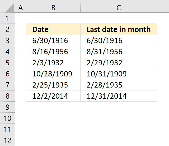
The formula in cell D3 calculates the last day for a given month based on a date in cell B3. The date is 1/1/2024, the last day in January 2024 is 31.

The way this works is that the formula adds one month to the date in cell B3 then subtracts with 1 to get the last date of the previous month.

Formula in cell C3:

=DATE(YEAR(B3),MONTH(B3)+1,1)-1

Back to top

Explaining formula in cell C3

Step 1 — Calculate year

The YEAR function returns a number representing the year based on an Excel date (serial number).

YEAR(serial_number)

YEAR(B3)

becomes

YEAR(1/1/2024)

becomes

YEAR(45292)

and returns 2024.

Step 2 — Calculate month

The MONTH function returns a number representing a month. 1 — January, …, 12 — December.

MONTH(serial_number)

MONTH(B3)+1

becomes

MONTH(45292)+1

becomes

1+1 equals 2.

Step 3 — Calculate day

The DAY function returns a number representing the day from an Excel date (serial number).

DAY(B3)

becomes

DAY(45292)

and returns 1.

Step 4 — Calculate the date

The DATE function calculates a serial number that represents a specific date based on three arguments. Year, month, and day.

DATE(year, month, day)

DATE(YEAR(B3),MONTH(B3)+1,1)-1

becomes

DATE(2014, 2, 1)-1

becomes

45323-1

and returns 45322 (1/31/2024).

Back to top

13. Get Excel file

Back to top

Calculate last date of a given month
The formula in cell C3 calculates the last date for the given month and year in cell B3. =DATE(YEAR(B3), MONTH(B3)+1, […]

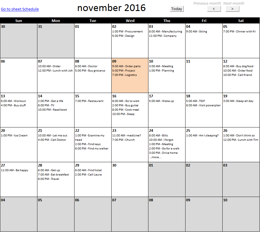
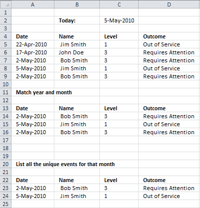
Calendar – monthly view
This article describes how to build a calendar showing all days in a chosen month with corresponding scheduled events. What’s […]

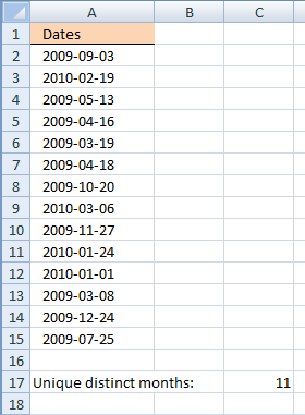
Count unique distinct months
The formula in cell D18 counts unique distinct months in cell range B3:B16. Formula in D18: =SUMPRODUCT((FREQUENCY(DATE(YEAR($B$3:$B$16), MONTH($B$3:$B$16), 1), DATE(YEAR($B$3:$B$16), […]

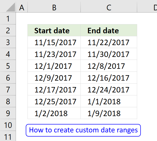
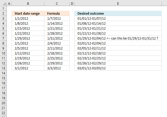
Create a date range [Formula]
Question: I am trying to create an excel spreadsheet that has a date range. Example: Cell A1 1/4/2009-1/10/2009 Cell B1 […]

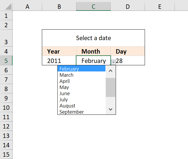
Create a drop down calendar
The drop down calendar in the image above uses a «calculation» sheet and a named range. You can copy the drop-down […]

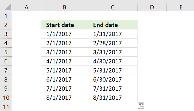
Create a monthly date range
I will demonstrate three different techniques to build monthly date ranges in this article. Two of these techniques are easy because they […]

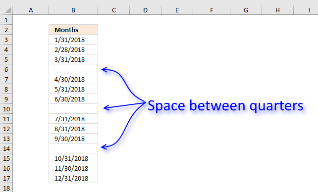
Create a quartely date range
I will demonstrate three different methods to build quarterly date ranges in this article. The two first methods have a […]

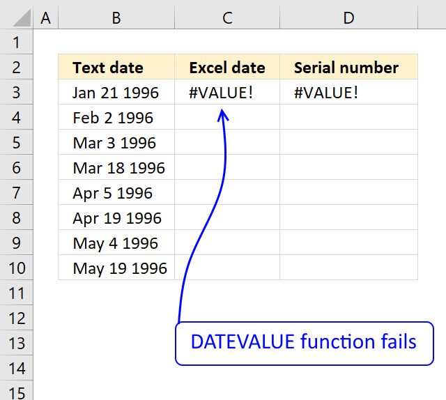
DATEVALUE function not working
The DATEVALUE function returns an Excel date value (serial number) based on a date stored as text. However, it must […]

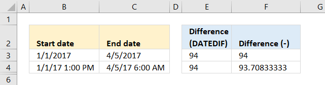
Days between two dates
The DATEDIF function in cell E3 allows you to calculate days between two dates.

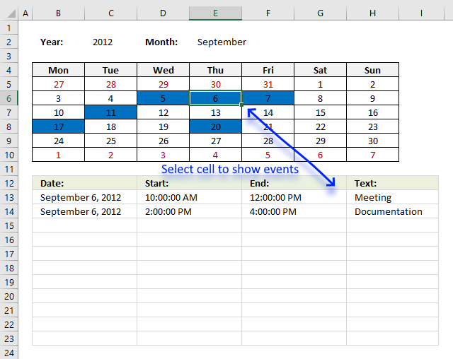
Excel calendar [VBA]
This workbook contains two worksheets, one worksheet shows a calendar and the other worksheet is used to store events. The […]

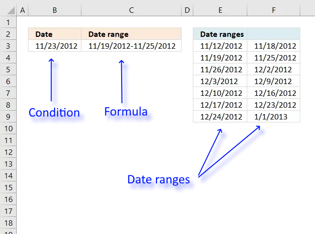
Find date range based on a date
This article demonstrates a formula that returns a date range that a date falls under, cell C3 above contains the […]

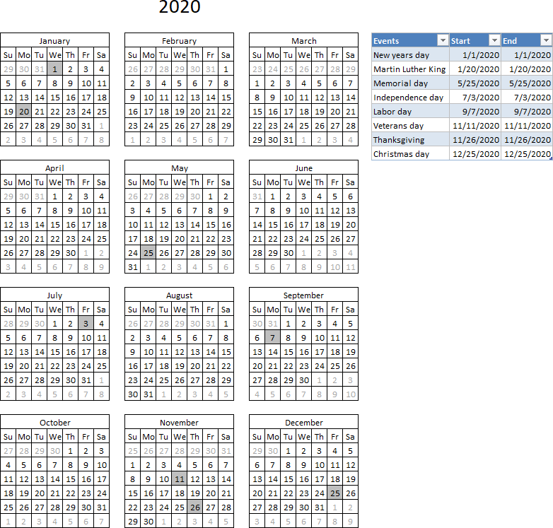
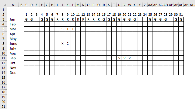
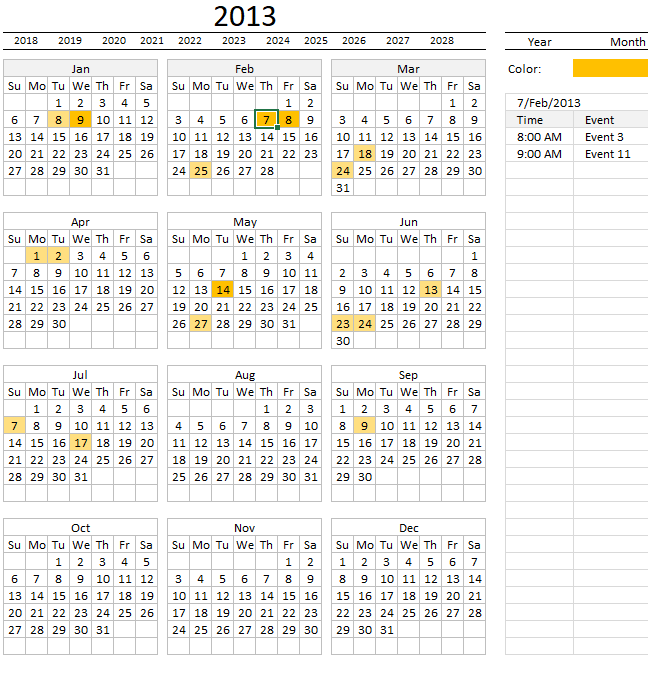
Highlight events in a yearly calendar
This article demonstrates how to highlight given date ranges in a yearly calendar, this calendar allows you to change the […]

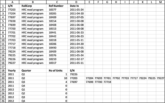
How to group items by quarter using formulas
This article demonstrates two formulas, the first formula counts items by quarter and the second formula extracts the corresponding items […]

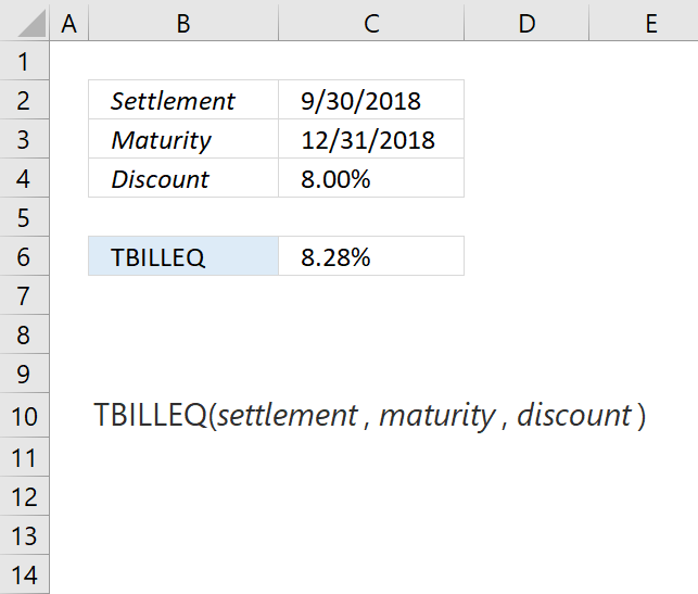
How to use the TBILLEQ function
The TBILLPRICE function calculates the equivalent bond yield for a Treasury bill. Formula in cell C6: =TBILLEQ(C2,C3,C4) Excel Function Syntax TBILLEQ(settlement, […]

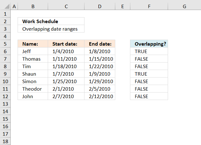
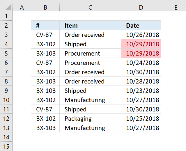
Identify overlapping date ranges
This article demonstrates formulas that show if a date range is overlapping another date range.  The second section shows how […]

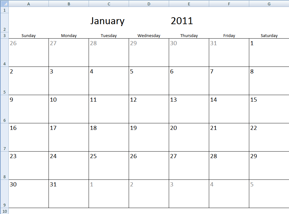
Monthly calendar template
The image above shows a calendar that is dynamic meaning you choose year and month and the calendar instantly updates […]

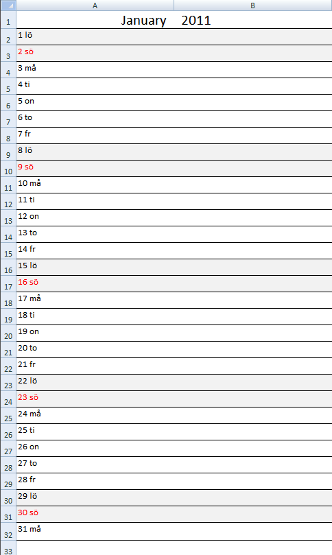
Monthly calendar template #2
I have created another monthly calendar template for you to get. Select a month and year in cells A1 and […]

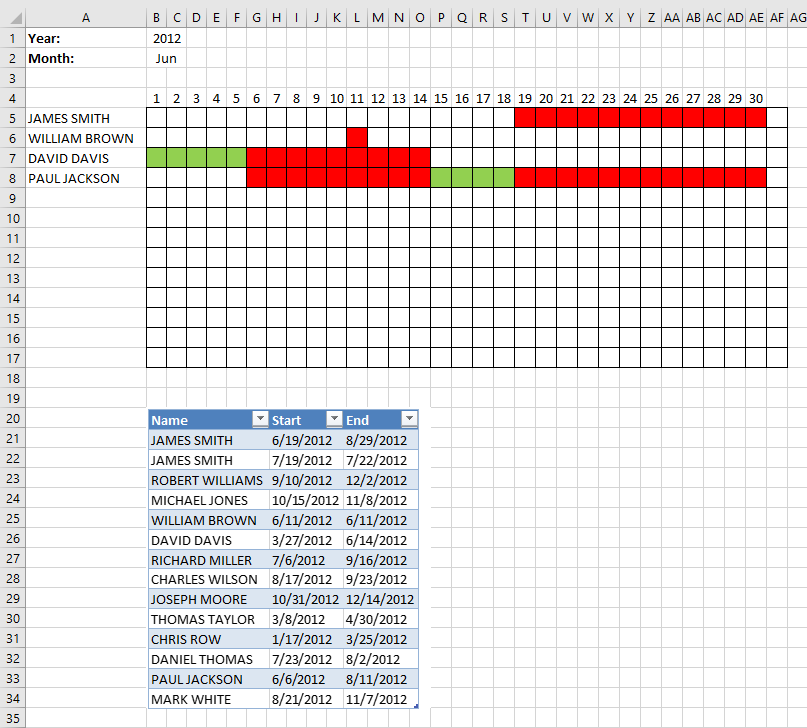
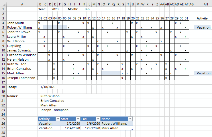
Plot date ranges in a calendar part 2
I will in this article demonstrate a calendar that automatically highlights dates based on date ranges, the calendar populates names […]

Yet another Excel Calendar
What’s on this page How to use this Excel Calendar How to add events How I built this calendar Worksheet […]

Returns a number that acts as a date in the Excel environment.

Returns the number of days, months, or years between two dates. The DATEDIF function exists in order to ensure compatibility with Louts 1-2-3.

Returns an Excel date value (serial number) based on a date stored as text.

Extracts the day as a number from an Excel date.

Calculates the number of days between two dates.

Returns a date determined by a start date and a number representing how many months.

Returns an Excel date for the last day of a given month using a number and a start date.

Returns an integer representing the hour of an Excel time value.

Returns a whole number representing the minute based on an Excel time value. The returned number is ranging from 0 to 59.

Extracts the month as a number from an Excel date.

Returns the number of working days between two dates, excluding weekends. It also allows you to ignore a list of holiday dates that you can specify.

Calculates the number of working days between two dates, excluding weekends.

Returns the current date and time.

Returns an integer representing the second based on an Excel time value

Returns a decimal value between 0 (zero) representing 12:00:00 AM and 0.99988426 representing 11:59:59 P.M.

Returns a decimal number based on a text string.

Returns the Excel date (serial number) of the current date.

Converts a date to a weekday number from 1 to 7.

Calculates a given date’s week number based on a return_type parameter that determines which day the week begins.

Returns a date based on a start date and a given number of working days (nonweekend and nonholidays).

Converts a date to a number representing the year in the date.

Returns the fraction of the year based on the number of whole days between a start date and an end date.

Excel functions that let you resize, combine, and shape arrays.

Functions for backward compatibility with earlier Excel versions. Compatibility functions are replaced with newer functions with improved accuracy. Use the new functions if compatibility isn’t required.

Perform basic operations to a database-like structure.

Functions that let you perform calculations to Excel date and time values.

Let’s you manipulate binary numbers, convert values between different numeral systems, and calculate imaginary numbers.

Calculate present value, interest, accumulated interest, principal, accumulated principal, depreciation, payment, price, growth, yield for securities, and other financial calculations.

Functions that let you get information from a cell, formatting, formula, worksheet, workbook, filepath, and other entitites.

Functions that let you return and manipulate logical values, and also control formula calculations based on logical expressions.

These functions let you sort, lookup, get external data like stock quotes, filter values based a condition or criteria, and get the relative position of a given value in a specific cell range. They also let you calculate row, column, and other properties of cell references.

You will find functions in this category that calculates random values, round numerical values, create sequential numbers, trigonometry, and more.

Calculate distributions, binomial distributions, exponential distribution, probabilities, variance, covariance, confidence interval, frequency, geometric mean, standard deviation, average, median, and other statistical metrics.

Functions that let you manipulate text values, substitute strings, find string in value, extract a substring in a string, convert characters to ANSI code among other functions.

Get data from the internet, extract data from an XML string and more.

Date and time in excel are treated a bit differently in excel than in other spreadsheets software. If you don’t know how Excel date and time work, you may face unnecessary errors.

So, in this article, we will learn everything about the date and time of Excel. We will learn, what are dates in excel, how to add time in excel, how to format date and time in excel, what are date and time functions in excel, how to do date and time calculations (adding, subtracting, multiplying etc. with dates and times).

What is Date and Time in Excel?

Many of you may already know that Excel dates and time are nothing but serial numbers. A date is a whole number and time is a fractional number. Dates in excel have different regional formatting. For example, in my system, it is mm/dd/YYYY (we will use this format throughout the article). You may be using the same date format or you could be using dd/mm/YYYY date format.

Date Formatting of Cell

There are multiple options available to format a date in Excel. Select a cell that may contain a date and press CTRL+1. This will open the Format Cells dialogue box. Here you can see two formatting options as Date and Time. In these categories, there are multiple date formattings available to suit your requirements.

Dates:

Dates in Excel are mare serial numbers starting from 1-Jan-1900. A day in excel is equal to 1. Hence 1-Jan-1900 is 1, 2-Jan-1900 is 2, and 1-Jan-2000 is 36526.

Fun Fact: 1900 was not a leap year but excel accepts 29-Feb-1900 as a valid date. It was a desperate glitch to compete Lotus 1-2-3 back in those days.

Shortcut to enter static today’s date in excel is CTRL+; (Semicolon).

To add or subtract a day from a date you just need to subtract or add that number of days to that date.

Time:
Excel by default follows the hh:mm format for time (0 to 23 format). The hours and minutes are separated by a colon without any spaces in between. You can change it to hh:mm AM/PM format. The AM/PM must have 1 space from the time value. To include seconds, you can add :ss to hh:mm (hh:mm:ss). Any other time format is invalid.

Time is always associated with a date. The date comes before the time value separated with a space from time. If you don’t mention a date before time, by default it takes the first date of excel (which is 1/1/1900). Time in excel is a fractional number. It is shown on the right side of the decimal.

Hours: 

Since 1 day is equal to 1 in excel and 1 day consists of 24 hours, 1 hour is equal to 1/24 in excel. What does that mean? It means that if you want to add or subtract 1 hour to time, you need to add or subtract 1/24. See the image below.

you can say that 1 hour is equal to 0.041666667 (1/24).

Calculate hours between time in Excel

Minutes:

From the explanation of the hour in excel, you must have guessed that 1 Minute in excel is equal to 1/(24×60) (or 1/1440 or 0.000694444).

If you want to add a minute to an excel time, add 1/(24×60). See the image below. Sometimes you get the need to Calculate Minutes Between Dates & Time In Excel, you can read it here.

Seconds:

Yes, a second in Excel is equal to 1/(24x60x60). To add or subtract seconds from a time, you just need to do the same things as we did in minutes and hours.

Date and Time in one cell

Dates and times are linked together. A date is always associated with a valid date and time is always associated with a valid excel date. Even if you are not able to see one of them.

If you only enter a time in a cell, the date of that cell will  1-Jan-1900, even if you are not able to see it. If you format that cell as a date-time format, you can see the associated date. Similarly, if you don’t mention time with the date, by default 12:00 AM is attached. See the image below.

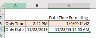
In the image above, we have time only in B3 and date only in B4. When we format these cells as mm/dd/yy hh:mm, we get both, time and date in both cells.

So, while doing date and time calculations in excel, keep this in check.

No Negative Time

As I told you the date and time in excel starts from 1-Jan-1900 12:00 AM. Any time before this is not a valid date in excel. If you subtract a value from a date that leads to before 1-Jan-1900 12:00, even one second, excel will produce ###### error. I have talked about it here and in Convert Date and Time from GMT to CST. It happens when we try to subtract something that leads to before 1 Jan-1900 12:00. Try it yourself. Write 12:00 PM and subtract 13 hours from it. see what you get.

Calculations with Dates and Time in Excel

Adding Days to a date:

Adding days to a date in excel is easy. To add a day to date just add 1 to it. See the image below.

You should not add two dates to get the future date, as it will sum up the serial numbers of those days and you may get a date far in the future.

Subtracting Days from Date:

If you want to get a backdate from a date a few days before, then just subtract that number of days from the date and you will get backdate. For example, if I want to know what date was before 56 days since TODAY then I would write this formula in the cell.

This will return us the date of 56 before the current date.
Note: Remember that you can not have a date before 1/Jan/1900 in excel. If you get ###### error, this could be the reason.

Days between two dates:
To calculate days between two dates we just need to subtract the start date from the end date. I have already done an article on this topic. Go and check it out here. You can also use the Excel DAYS Function to calculate days between a start date and end date.

Adding Times:
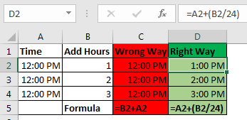
There’s been a lot of queries on how to add time to excel as many people get confusing results when they do it. There are two types of addition in times. One is adding time to another time. In this case, both times are formatted as hh:mm time format. In this case, you can simply add these times.

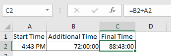
The second case is when you don’t have additional time in time format. You just have numbers of hours, minutes and seconds to add. In that case, you need to convert those numbers to their time equivalents. Note these points to add hours, minutes and seconds to a date/time.

• To add N hours to an X time use formula =X+(N/24) (As 1=24 hours)
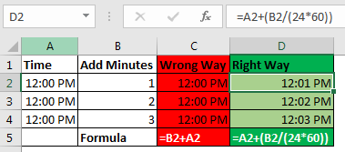
• To Add N minutes to X time use formula = X+(N/(24*60))
• To Add N Second to X time use formula = X+(N/(24*60*60))

Subtracting Times

It’s the same as adding time, just make sure that you don’t end up with a negative time value when subtracting, because there is no such thing as a negative number in excel.

Note: When you add or subtract time in excel that exceeds 24 hours of difference, excel will roll to the next or previous date. For example, if you subtract 2 hours from 29-Jan-2019 1:00 AM then it will roll back to 28-Jan-2019 11:00 PM. If you subtract 2 hours from 1:00 AM (does not have the date mentioned), Excel will return ###### error. I have told the reason at the beginning of the article.

Adding Months to a Date:

You can’t just add multiples of 30 to add months to date as different months have a different number of days. You need to be careful while adding months to Date. To add months to a date in excel, we use EDATE function of excel. Here I have a separate article on adding months to a date in different scenarios.

Adding years to date:

Just like adding months to a date, it is not straightforward to add years to date. We need to use YEAR, MONTH, DAY function to add years to date. You can read about adding years to date here.

If you want to calculate years between dates then you can use this.

Excel Date and Time Handling Functions:

Since date and time are special in Excel, Excel provides special functions to handle them. Here I am mentioning a few of them.

1. TODAY(): This function returns today’s date dynamically.
2. DAY(): Returns Day of the month (returns number 1 to 31).
3. DAYS(): Used to count the number of days between two dates.
4. MONTH(): Used to get the month of the date (returns number 1 to 12).
5. YEAR(): Returns year of the date.
6. WEEKNUM(): Returns the weekly number of a date, in a year.
7. WEEKDAY(): Returns the day number in a week (1 to 7) of the supplied date.
8. WORKDAY():  Used to calculate working days.
9. TIMEVALUE(): Used to extract Time value (serial number) from a text formatted date and time.
10. DATEVALUE(): Used to extract date value (serial number) from a text formatted date and time.

These are some of the most useful data and time functions in excel. There are plenty more date and time functions. You can check them out here.

Date and Time Calculations

If I explain all of them here, this article will get too long. I have divided these time calculation techniques in excel into separate articles. Here I am mentioning them. You can click on them to read.

• Calculate days, months and years
• Calculate age from date of birth
• Multiplying time values and numbers.
• Get Month name from Date in Excel
• Get day name from Date in Excel
• How to get a quarter of the year from date
• How to Add Business Days in Excel
• Insert Date Time Stamp with VBA

So yeah guys, this is all about the date and time in excel you need to know about. I hope this article was useful to you. If you have any queries or suggestions, write them down in the comments section below.

For work with dates in Excel, in the category «Date and time» is defined in the functions section. Let`s consider the most prevalent functions in this category.



How Excel Processes Time

The Excel program «perceives» the date and time as an ordinary number. The spreadsheet converts to such number, equating the day to unity. As a result, the time value represents a fraction of unity. For example, 12. 00 — is 0. 5.

The date value to the spreadsheet converts to a number which equal to the number of days from January 1, 1900 (so the developers decided) to the specified date. For example, when converting the date 13. 04. 1987, the number is 31880. That is, from 1. 01. 1900 passed 31. 880 days.

This principle underlies in the basis of the calculations of the time data. To find the number of days between two dates, it`s enough to take an earlier period from a later time one.



The example of DATE function

You need to describe of the date value with compiling it with individual elements of numbers.

There is the syntax: year; month, day.

All arguments are required. They can be specified by numbers or by reference to cells with the corresponding numeric data: for the year — from 1900 to 9999; for the month — from 1 to 12; for the day — from 1 to 31.

If you point a larger number for the «Day» argument (than the number of days in the pointed month), you receive the extra days, will be passed to the next month. For example, specifying 32 days for December, we will receive as a result on January 1.

The example of using the function:

Let’s set more days for June:

Examples of using the cell references as arguments:

The DATEDIF function in Excel

It returns the difference between two dates.

The arguments:

• start date;
• final date;
• the code indicating to the units of counting (days, months, years, etc.).

The methods of measuring intervals between the given dates:

• to display the result in days — «d»;
• in months – «m»;
• in years – «y»;
• in months without years – «ym»;
• in days without months and years – «md»;
• in days without years – «yd».

In some versions of Excel, if you use the last two arguments («md», «yd»), the function may give an error. It is better to use to alternative formulas.

The examples of the operation the DATEDIF function:

In Excel 2007 version, this function is not in the directory, but it works. But you need to check the results are better, because there are flaws possible.

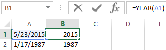
The YEAR function in Excel

It returns the year as an integer number (from 1900 to 9999), what corresponds to the specified date. There is only one argument must be entered in the structure of the function – is the date in a numerical format. The argument must be entered using the DATE function or represents to the result of evaluating other formulas.

The example of using the YEAR function:

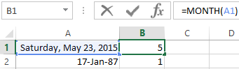
The MONTH function in Excel: the example

It returns the month as an integer number (from 1 to 12) for a date is specified in a numeric format. The argument – is the date of the month that you want to show in a numerical format. The dates in the text format this function does not handle correctly.

The examples of using the MONTH function:

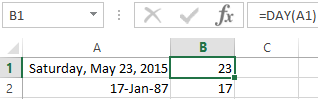
The examples of DAY, WEEKDAY and functions WEEKNUM in Excel

It returns the day as an integer number (from 1 to 31) for a date specified in a numeric format. The argument – it is the date of the day you want to find in a numerical format.

For returning of the weekday ordinal of the specified date, you can apply the function WEEKDAY:

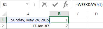
By default, the function considers Sunday the 1-st day of the week.

To display of the ordinal number of the week for the pointed date, you should use the WEEKNUM function:

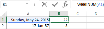
The date of 24. 05. 2015 is 22 week in a year. The week starts on Sunday (by default).

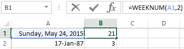
As the second argument the figure 2 is specified. Therefore, the formula considers that the week starts on Monday (the 2-d day of the week).

Download all examples functions for working with dates

For indicating of the current date, the function TODAY (no arguments) is used. To display the current time and date, the function NOW() is used.

Sample Files

1. DATE Function

DATE function returns a valid date based on the day, month, and year you input. In simple words, you need to specify all the components of the date and it will create a date out of that.

Syntax

DATE(year,month,day)

Arguments

• year: A number to use as the year.
• month: A number to use as the month.
• day: A number to use as a day.

Example

In the below example, we have used cell references to specify the year, month, and day to create a date.

You can also insert arguments directly into the function to create a date as you can see in the below example.

And in the below example, we have used different types of arguments to see the result returned by the function.

2. DATEVALUE Function

DATEVALUE function returns a date after converting a text (which represents a date) into an actual date. In simple words, it converts a date into an actual date which is formatted as text.

Syntax

DATEVAUE(date_text)

Arguments

• date_text: The date which is stored as a text and you want to convert that text into an actual date.

Example

In the below example, we have inserted a date directly into the function by using double quotation marks. If you skip adding these quotation marks it will return a #NAME? error in the result.

In the below example, all the dates on the left side are in textual format.

1. A simple textual date that we have converted into a valid date.
2. A date with all three components (Year, Month, or Day) in numbers.
3. If there is no year in the textual date, it will take the current year as the year.
4. And if you have a month name is in alphabets and no year, it will take the current year as a year.
5. If you don’t have the day in your textual date it will take 1 as the day number.

3. DAY Function

DAY function returns the day number from a valid date. As you know, in Excel, a date is a combination of day, month, and year, DAY function gets the day from the date and ignores the rest of the part.

Syntax

DAY(serial_number)

Arguments

• serial_number: A valid serial number of the date from which you want to extract the day number.

Example

In the below example, we have used the DAY to simply get the day from a date.

And in the below example, we have used DAY with TODAY to create a dynamic formula that returns the current day number and it will update every time you open your worksheet or when you recalculate your worksheet.

5. DAYS Function

DAYS function returns the difference between two dates. It takes a start date and an end date and then returns the difference between them in days. This function was introduced in Excel 2013 so not available in prior versions.

Syntax

DAYS(end_date,start_date)

Arguments

• start_date: It is a valid date from where you want to start the days’ calculation.
• end_date: It is a valid date from where you want to end the days’ calculation.

Example

In the below example, we have referred the cell A1 as the start date and B1 as the end date and we have 9 days in the result.

Note: You can also use the subtract operator to get the difference between two dates.

In the below example, we have directly inserted two dates into the function to get the difference between them.

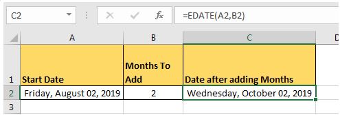
6. EDATE Function

EDATE function returns a date after adding a specified number of months to it. In simple words, you can add (with a positive number) or subtract (with a negative number) months from a date.

Syntax

EDATE(start_date,months)

Arguments

• start_date: The date from which you want to start the calculation.
• months: The number of months to calculate the future or the past date.

Example

Here we have used EDATE with different types of arguments.

• In the first example, we have used 5 as a several months and it has added exactly 5 months on 1-Jan-2016 and returned 01-June-2016.
• In the second example, we have used -1 month and it has given 31-Dec-2016, a date which is exactly 1 month back from 31-Jan-2016.
• In the third example, we have inserted a date directly into the function.

7. EOMONTH Function

EOMONTH function returns the end of the month date which is the number of months in the future or the past. You can use a positive number for a future date and a negative number for the past month’s date.

Syntax

EOMONTH(start_date,months)

Arguments

• start_date: A valid date from where you want to start your calculation.
• months: The number of months you want to calculate before and after the start date.

Example

In the below example, we have used EOMONTH with different types of arguments:

• We have mentioned 01-Jan-2016 as the start date and 5 months for getting a future date. As June is exactly 5 months after January, it has returned 30-Jun-2016 in the result.
• As I have already mentioned, EOMMONTH is smart enough to evaluate the total number of days in a month.
• If you mention a negative number, it simply returns a past date which is the number of months back you have mentioned.
• In the fourth example, we have used a date that is in text format and it has returned the date without returning any errors.

8. MONTH Function

MONTH function returns the month number (ranging from 0 to 12) from a valid date. As you know, in Excel, a date is a combination of day, month, and year, MONTH gets the month from the date and ignores the rest of the part.

Syntax

MONTH(serial_number)

Arguments

• serial_number: A valid date from which you want to get the month number.

Example

In the below example, we have used a MONTH in three different ways:

• In the FIRST example, we have simply used date and it has returned the 5 in the result which is the month number of MAY.
• In the SECOND example, we have supplied the date directly in the function.
• In the THIRD example, we have used the TODAY function to get the current date and MONTH has returned the month number from it.

9. NETWORKDAYS Function

NETWORKDAYS function returns the count of days between the start date and end date. In simple words, with NETWORKDAYS you can calculate the difference between two dates, after excluding Saturdays and Sundays, and holidays (which you specify).

Syntax

NETWORKDAYS(start_date,end_date,holidays)

Arguments

• start_date: A valid date from where you want to start your calculation.
• end_date: A valid date up to which you want to calculate working days.
• [holidays]: A valid date that represents a holiday between the start date and end date. You can refer to a cell, range of cells, or an array containing dates.

Example

In the below example, we have specified 10-Jan-2015 as a start date and 20-Feb-2015 as an end date.

We have 41 days between these two dates, out of which 11 days are weekends. After deducting those 11 days it has returned 30 working days.

Now in the below example with the same start and end dates, we have specified a holiday and, after deducting 11 days of the weekend and 1 holiday it has returned 29 working days.

Again with the same start and end dates, we have used a range of three cells for holidays to deduct from the calculation and, after deducting 11 weekend days and 3 holidays which I have mentioned It has returned 27 working days.

10. NETWORKDAYS.INTL Function

NETWORKDAYS.INTL Function returns the count of days between the start date and end date. Unlike NETWORKDAYS, NETWORKDAYS.INTL lets you specify which days you want to exclude from the calculation.

Syntax

NETWORKDAYS.INTL(start_date,end_date,weekend,holidays)

Arguments

• start_date: A valid date from where you want to start your calculation.
• end_date: A valid date up to which you want to calculate working days.
• [weekend]: A number represents to exclude weekends from the calculation.
• [holidays]: A list of dates that represents the holidays you want to exclude from the calculation.

Example

In the below example, we have used 01-Jan-2015 as a start date and 20-Jan-2015 as an end date. And we have specified 1 to take Sunday – Saturday as the weekend. The function has returned 14 days after excluding 6 weekend days.

Below, we have used the same dates. And I have used 11 in for weekend days which means it will only consider Sunday as a weekend. Along with that, we have also used 10-Jan-2015 as a holiday.

We have 3 Sundays between both dates and a holiday. After excluding all these days the function has returned 16 days in the result. Here in the below example, we have used range to specify holidays. If you have more than one date for the holidays you can refer to an entire range.

Quick Tip: If you want to create a dynamic range for holidays, you can use a table for that. If you want to choose custom days to count as working days or weekends, you can use the below format in the weekend argument.

Here, 0 represents a working day and 1 represents a non-working day. And, seven numbers represent 7 days of the week.

11. TODAY Function

The TODAY function returns the current date and time as per the system’s date and time. The date and time returned by the NOW function update continuously whenever you update anything in the worksheet.

Syntax

TODAY()

Arguments

• In the TODAY function, there is no argument, all you need to do is enter it in the cell and hit enter, but be careful as TODAY is a volatile function which updates its value every time you update your worksheet calculations.

Example

In the below example, we have used TODAY  with other functions to get the current month number, current year, and current day.

12. WEEKDAY Function

WEEKDAY function returns a day number (ranging from 0 to 7) of the week from a date. In simple words, the WEEKDAY function takes a date and returns the day number of that date’s day.

Syntax

WEEKDAY (serial_number, [return_type])

Arguments

• serial_number: A valid date from which you want to get the week number.
• [return_type]: A number that represents the day of the week to start the week.

Example

In the below example, we have used a WEEKDAY with TODAY to get a dynamic weekday. It will give you the weekday whenever the current date changes. You can use this method in your dashboards to trigger some values which need to change when weekday change.

In the below example, we have used WEEKDAY with IF to create a formula that first checks the weekday of date and return “Weekday” or “Weekend” basis on the value return from WEEKDAY.

13. WEEKNUM Function

WEEKNUM function returns the week number of a date. In simple words, WEEKNUM returns the week number of dates that you specify ranging from 1 to 54.

Syntax

WEEKNUM(serial_number,return_type)

Arguments

• serial_number: A date for which you want to get the week number.
• [return_type]: A number to specify the starting day of the first week of the year. You have two systems to specify the starting date of the week.

Example

In the below example, we have used TODAY with WEEKNUM to get the week number of the current date. It will update the week number automatically every time the date changes.

In the below example, we have added the text “Week-” with the week number for a meaningful result.

14. YEAR Function

YEAR Function returns the year number from a valid date. As you know, in Excel a date is a combination of day, month, and year, and the YEAR function gets the year from the date and ignores the rest of the part.

Syntax

YEAR(date)

Arguments

• date: A date from which you want to get the year.

Example

In the below example, we have used the year function to get the year number from the dates. You can use this function where you have dates in your data and you only need the year number.

And in the below example, we have used today function to get the year number from the current date. It will always update the year whenever you recalculate your worksheet.

---

Bottom line: With Valentine’s Day rapidly approaching I thought it would be good to explain how you can get a date with your Excel skills.  Just kidding! 🙂  This post and video explain how the date calendar system works in Excel.

Skill level: Beginner

Dates in Excel can be just as complicated as your date for Valentine’s Day.  We are going to stick with dates in Excel for this article because I’m not qualified to give any other type of dating advice. 🙂

Video Tutorial on How Dates Work in Excel

The following is a video from The Ultimate Lookup Formulas Course on how the date system works in Excel.

Watch the Video on YouTube

There are over 100 short videos just like the one above included in the Ultimate Lookup Formulas Course.

This course has been designed to help you master Excel’s most important functions and formulas in an easy step-by-step manner.

The Ultimate Lookup Formulas course is now part of our comprehensive Elevate Excel Training Program.

Click Here to Learn More About Elevate Excel

What is a Date in Excel?

I should first make it clear that I am referring to a date that is stored in a cell.

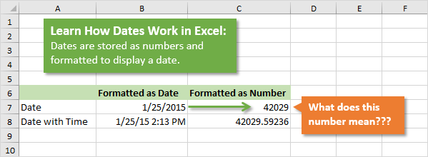
The dates in Excel are actually stored as numbers, and then formatted to display the date.  The default date format for US dates is “m/d/yyyy” (1/27/2016).

The dates are referred to as serial numbers in Excel.  You will see this in some of the date functions like DAY(), MONTH(), YEAR(), etc.

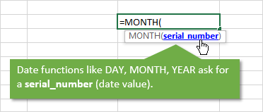
So then, what is a serial number?  Well let’s start from the beginning.

The date calendar in Excel starts on January 1st, 1900.  As far as Excel is concerned this day starts the beginning of time.

Each Day is a Whole Number

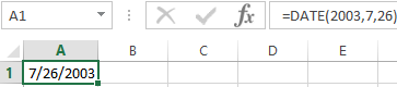
Each day is represented by one whole number in Excel.  Type a 1 in any cell and then format it as a date.  You will get 1/1/1900.  The first day of the calendar system.

Type a 2 in a cell and format it as a date.  You will get 1/2/1900, or January 2nd.  This means that one whole day is represented by one whole number is Excel.

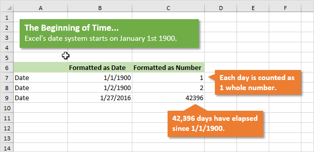
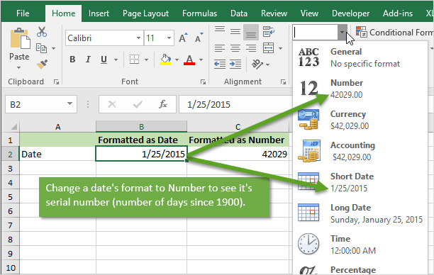
You can also take a cell that contains a date and format it as a number.

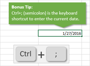
For example, this post was published on 1/27/2016.  Put that number in a cell (the keyboard shortcut to enter today’s date is Ctrl+;), and then format it as a number or General.

You will see the number 42,396.  This is the number of days that have elapsed since 1/1/1900.

Date Based Calculations

It is important to know that dates are stored as the number of days that have elapsed since the beginning of Excel’s calendar system (1/1/1900).

When you calculate the difference between two dates by subtraction, the result will be the number of days between the two dates.

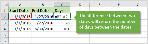
1/27/2016 – 1/1/2016 = 26 days

6/30/2016 – 1/1/2016 = 181 days

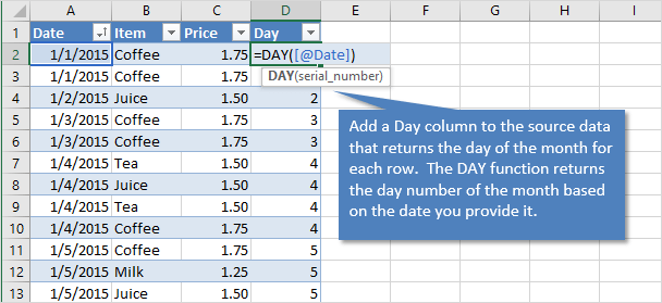
There are a lot of Date functions in Excel that can help with these calculations.  Last week we learned about the DAY function for month-to-date calculations with pivot tables.

We won’t go into all the date functions here, but understanding that the serial number represents one day will give you a good foundation for working with dates.

What About Dates with Times?

Do you ever work with dates that contain time values?

These dates are still stored as serial numbers in Excel.  When you convert the date with a time to the number format, you will see a decimal number.

This decimal is a fraction of the day.

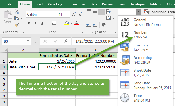
One hour in Excel is represented by the number: 1/24 = 0.04167

One minute in Excel is represented by the number: 1/(24*60) = 1/1440 = 0.000694

So 8:30 AM can be calculated as: (8 * (1/24)) + (30 * (1/1440)) = .354167

An easier way to calculate this is by typing 8:30 AM in a cell, then changing the format to Number.

So if you are running a half hour late and want to let your boss know, text him/her and say you will be there at 0.354167. 🙂

Checkout my article on 3 ways to group times in Excel for more date time based calculations.

Don’t Talk About Excel Dates with Your Date

Unless your Valentine shares a similar passion for Excel, I strongly recommend NOT sharing this information on your date.

I remember the first time I met my wife, and told her I worked in finance.  The first word out of her mouth was, “BORING!”.  Awe… it was love at first sight… LOL 🙂

But you should now be able to use Excel to determine how many days it has been since you last spoke to your date.  That’s the only dating advice I can give.

Please leave a comment below with any questions on Excel dates.  Thanks!

In This Chapter

Understanding how Excel handles dates
Formatting dates
Working with days, months, and years
Getting the value of Today Determining the day of the week
When working with Excel, you need to manage dates. Perhaps you have list of dates when you visited a client and you need to count how many times you were there in September. On the other hand, maybe you are tracking a project over a few months, and want to know how many days are in between the milestones.
Excel has a number of useful Date functions to make your work easier! This chapter explains how to work with parts of a date, such as the month or year, and even how to count the number of days between two dates. You can always reference the current data from your computer’s clock and use it in a calculation.

Understanding How Excel Handles Dates

Imagine if, on January 1, 1900, you starting counting by ones, each day adding one more to the total. This is just how Excel thinks of dates. January 1, 1900, is one; January 2, 1900, is two; and so on. We’ll always remember 25,404 as the day man first walked on the moon, and 36,892 as the start of the new millennium!

The millennium actually started on January 1, 2001. The year 2000 is the last year of the 20th century.

Excel represents dates as a serial number — specifically, the number of days between January 1, 1900, and the date in question. Excel can handle dates from January 1, 1900 to December 31, 9999. Using the serial numbering system,that’s 1 through 2,958,465!
Because Excel represents dates in this way, it can work with dates in the same manner as numbers. For example, you can subtract one date from another to find out how many days are between them. Likewise, you can add 14 to today’s date to get a date two weeks in the future. This trick is very useful but people are used to seeing dates represented in traditional formats, not as numbers. Fortunately, Excel has the tools for date formatting as well.

In Excel for the Mac, the serial numbering system begins on January 1, 1904.

The way years are handled requires special mention. When a year is fully displayed in four digits, such as 2005, there is no ambiguity. However, when a date is written in a shorthand style, such as in 3/1/02, it isn’t clear what the year is. It could be 2002, or it could be 1902. Let’s say 3/1/02 is a shorthand entry for someone’s birthday. Then on March 1, 2005, he is either 3 years old or 103 years old. In some countries this would be January 3, 1902 or January 3, 2002.
Excel and the Windows operating system have a default way of interpreting shorthand years. Windows 2000 and later has a setting in the Customize Regional Options dialog box found in the Control Panel. Here’s how to open and set it:
1. Click on your computer’s Start button.
2. Select Control Panel.
3. Select Regional and Language Options.
4. In the Regional and Language Options dialog box, select the Regional Options tab if it is not selected by default.
5. Click the Customize button.
The Customize Regional Options dialog box appears.
6. Select the Date tab in the Customize Regional Options dialog box.
7. Enter a four-digit ending year (such as 2029) to indicate the latest year that will be used when interpreting a two-digit year.
8. Click OK to close each dialog box.
This setting guides how Excel will interpret years. So if the setting is 1930 through 2029, then 3/1/02 indicates the year 2002, but 3/1/45 indicates the year 1945, not 2045. Figure 12-1 shows this setting.

Figure 12-1:
Setting how years are interpreted.
To ensure full accuracy when working with dates, always enter the full four digits for the year.

Formatting Dates

When you work with dates, you’ll probably need to format cells in your worksheet. It’s great that Excel tells you that June 1, 2005, is serially represented as 38504, but we don’t think that’s what you want on a report. To format dates, you use the Format Cells dialog box, shown in Figure 12-2. To format dates, follow these steps:
1. Choose Format O Cells.
The Format Cells dialog box appears.
2. Select the Number tab in the Format Cells dialog box if it is not already selected.
3. Select Date in the Category List.
4. Select an appropriate format in the Type List.
Now you can turn the useful but pesky serial dates into a user-friendly format.

Figure 12-2:
Using the Format Cells dialog box to control how dates are displayed.

Assembling a Date with the DATE Function

You can use the DATE function to create a complete date when you have separate year, month, and day information. The DATE function can be useful because dates don’t always appear as, well, dates, in a worksheet. You may have a column of values between 1 and 12 that represents the month, and another column of values between 1 and 31 for the day of the month. A third column may hold years — in either the two-digit shorthand or the full four digits.

The DATE function combines individual day, month, and year components into a single usable date. This makes using and referencing dates in your worksheet easy. To use the DATE function:

1. Select the cell where you want the results displayed.
2. Enter =DATE( to begin the function entry.
3. Click the cell that has the year.
4. Enter a comma (,).
5. Click the cell that has the number (1-12) that represents the month.
6. Enter a comma (,).
7. Click the cell that has the number (1-31) that represents the day of the month.
8. Enter a closing parenthesis to end the function, and press Enter.
Figure 12-3 displays a fourth column of dates that are created using DATE and the values from the first three columns. The fourth column of dates has been formatted so the dates are displayed in a standard format, not as a raw date serial number.

Figure 12-3:
Using the DATE function to assemble a date from separate month, day, and year values.

Breaking Apart a Date with the DAY, MONTH, and YEAR Functions

That which can be put together can also be taken apart. In the preceding section, we show you how to use the DATE function to create a date from separate year, month, and day data. In this section, you find out how to do the reverse — split a date into individual year, month, and day components using the DAY, MONTH, and YEAR functions. In Figure 12-4, the dates in column A are split apart by day, month, and year, respectively, in columns B, C, and D.

Isolating the day with the DAY function

Isolating the day part of a date is useful in applications where just the day, but not the month or year, is relevant. For example, say you own a store and want to figure out if more customers come to shop in the first half or the second half of the month. You’re interested in this trend over several months. So the task may be to average the number of sales by the day of the month only.

Figure 12-4:
Splitting apart a date with the DAY, MONTH, and YEAR functions.
The DAY function is useful for this because you can use it to return just the day for a lengthy list of dates. Then you can examine results by the day only.

Here’s how you use the DAY function:

1. Position the mouse in the cell where you want the results displayed.
2. Enter =DAY( to begin the function entry.
3. Click the cell that has the date.
4. Enter a closing parenthesis to end the function, and press Enter.

Excel returns a number between 1 and 31.

Figure 12-5 shows how the DAY function can be used to analyze customer activity. Column A contains a full year’s sequential dates. In Column B, the day part of each date has been isolated. Column C shows the customer traffic for each day.
This is all the information that is needed to analyze whether there is a difference in the amount of customer traffic between the first half and second half of the month.
Cells E4 and E10 show the average daily customer traffic for the first half and second half of the month, respectively. The value for the first half of the month was obtained by adding all the customer values for those day values in the range 1 to 15, and then dividing by the total number of days. The value for the second half of the month was done the same way, but using day values in the range 16 to 31.

Figure 12-5:
Using the DAY function to analyze customer activity.
The day parts of the dates, in Column B, were key to these calculations:
‘ In cell E4 the calculation is =SUMIF(B2:B367,”<16″,C2:C367)/COUNT IF(B2:B367″<16″).
‘ In cell E10 the calculation is =SUMIF(B2:B367,”>15″,C2:C367)/COUNT IF(B2:B367,”>15″).
The SUMIF function is discussed in Chapter 7. The COUNTIF function is discussed in Chapter 11.
The DAY function has been instrumental in showing that more customers visit the fictitious store in the second half of the month. This type of information is great for a store owner to plan staff assignments, sales specials, and so on.

Isolating the month with the MONTH function

Isolating the month part of a date is useful in applications where just the month, but not the day or year, is relevant. For example, you may have a list of random dates and need to determine the number of dates that fall in each of the 12 months.
You could sort the dates and then count the number for each month. That would be easy enough, but sorting may not be an option based on other requirements. Besides, why manually count when you have right in front of you one of the all-time greatest counting software programs ever made!
Figure 12-6 shows a worksheet in which the MONTH function has been used to extract the numeric month value (1-12) into Column B from the dates in Column A. Cell B2 contains the formula =MONTH(A2) and so on down the column. Columns C and D contain a summary of dates per month. The formula used in cell D3 is:

This counts the number of dates where the month value is 1. Cells D4 through D14 contain similar formulas for month values 2 through 12.

Figure 12-6:
Using the MONTH function to count the number of dates falling in each month.

See Chapter 14 for information on the COUNTIF function.

In Figure 12-6, the dates in Column A are random, so discerning much about the dates is difficult. However, the summary, as well as the chart based on the summary, show that more dates appear in the winter months (assuming you’re in the Northern Hemisphere).

To use the MONTH function:

1. Select the cell where you want the results displayed.
2. Enter =MONTH( to begin the function entry.
3. Click the cell that has the date.
4. Enter a closing parenthesis to end the function, and press Enter.
Excel returns a number between 1 and 12.

Isolating the year with the YEAR function

Isolating the year part of a date is useful in applications where just the year, but not the day or month, is relevant. In practice, this is less used than the DAY or MONTH functions because date data is often — though not always — from the same year.

To use the YEAR function:

1. Select the cell where you want the results displayed.
2. Enter =YEAR( to begin the function entry.
3. Click the cell that has the date.
4. Enter a closing parenthesis to end the function, and press Enter.
Excel returns the four-digit year.

Using DATEVALUE to Convert a Text Date into a Numerical Date

You may have data in your worksheet that looks like a date but is not represented as an Excel date value. For example, you could enter the text “01-14-04″ in a cell, and Excel would have no way of knowing whether this is January 14, 2004, or the code for your combination lock. Don’t tell anyone! But if it looks like a date, you can use the DATEVALUE function to convert it into an Excel date value.
Why not enter dates as text data? Because although they may look fine, you can’t use them for any of Excel’s powerful date calculations without first converting them to date values.
The DATEVALUE function recognizes almost all commonly used ways that dates are written. Here are some ways that people may enter August 5, 2005:
8/5/05
5-Aug-2005 2005/08/05
DATEVALUE can convert these and several other date representations to a date serial number.
After you’ve converted the dates to a date serial number, the dates can be used in other date formulas or to perform calculations as described in other parts of this chapter.

To use the DATEVALUE function, follow these steps:

1. Select the cell where you want the date serial number located.
2. Enter =DATEVALUE( to begin the function entry.
3. Click the cell that has the text format date.
4. Enter a closing parenthesis to end the function, and press Enter.
The result will be a date serial number, unless the cell where the result is displayed has already been set to a date format.
Figure 12-7 shows how some nonstandard dates in Column A have been converted with the DATEVALUE function.

Figure 12-7:
Converting dates into their serial equivalents with the DATEVALUE function.
Did you notice something funny in Figure 12-7? Normally, you won’t be able to enter a value such as the one in cell A4 — 02-28-06 — without losing the leading zero. The cells in Column A had been changed to the Text format. This format tells Excel to leave your entry as it is. The Text format is one of the choices in the Category list in the Format Cells dialog box (refer to Figure 12-2).
In reality, you won’t need DATEVALUE too often because Excel is pretty good at recognizing dates that you enter in the standard formats. If, for example, you enter “12/5/04″ in a cell, Excel recognizes that this is meant as a date and not as text. It’s automatically converted to a date serial number and displayed using the default date format. DATEVALUE is used most often when you’re importing text data from another application and Excel fails to perform the automatic conversion.
Please look back at Figure 12-7, specifically at cell B8. Excel could not figure out how to interpret the Feb 9 05 value in cell A8. Therefore, cell B8 shows an error. We did say Excel is great at recognizing dates, but we did not say it is perfect! In cases such as this, you’ll have to edit the date to put it into a format that DATEVALUE can recognize.

Using the TODAY Function to Find Out the Current Date

Often, when working in Excel, you need to use the current date. Each time a worksheet is printed, for example, you may want it to show the date it was printed. The TODAY function fills the bill perfectly for this. TODAY simply get the date from your computer’s internal clock. To use the TODAY function, follow these steps:
1. Position the mouse to the cell where you want the result.
2. Type =TODAY( ).
3. Press Enter to end the function.
That’s it! You now have the date from your computer. If your computer’s clock is not set correctly, don’t blame Excel. Like all dates in Excel, what you really end up with is a serial number, but the Date formatting displays the date in a readable fashion.
As with all functions in Excel, you can embed functions in other functions. So, for example, if you need to know just the month of the current date, you can combine the TODAY function with the MONTH function, like this:

Counting the number of days until Christmas

Have a bit of shopping left to do for the holidays? Excel can help keep track of how many days are left. Remember that Excel is able to perform mathematical operations on dates. So let Excel do the counting. This formula, entered in a cell, tells you how many days are left until Christmas 2005:

The formula assumes you’re counting days in the year 2005. Change the year reference as needed.
The DATE function is used to enter the day, month, and year of Christmas. This avoids having a shorthand entry, such as 12/25/2005 be interpreted as a mathematical operation on its own.
If the entry was =12/25/2005 – TODAY(), an incorrect answer would be calculated; because this effectively says, “Divide 12 by 25, then divide that result by 2005, then subtract the serial number of today’s date.” The answer would be incorrect.
Using the DATE function to represent dates in which a mathematical operation is performed is a good idea.

Counting your age, in days

Sometimes you’re asked how old you are. Maybe you’d rather not say. Here’s a way to tell but in a way that will still leave the person who asked you unsure of the answer. Answer by saying how old you are in days!
Excel can help figure this out. All you have to do is count the number of days between your birth date and the current date. A simple formula tells you this:

Just substitute your real birth year, month, and day into the formula.

Determining the Day of the Week with the WEEKDAY Function

The Beatles wrote a song called “Eight Days a Week,” but for the rest of us seven days is the norm. The WEEKDAY function helps you figure out which day of the week a date falls on. Using this function, you can find out what day of the week an upcoming event will occur on, such as what day your birthday will fall on next year.

Here is how you use the WEEKDAY function:

1. Select the cell where you want the results displayed.
2. Enter =WEEKDAY( to begin the function entry.
3. Select the cell that has the date you want to find out the weekday for.
4. Enter a closing parenthesis to end the function, and press Enter.
WEEKDAY returns a number between 1 and 7. Table 12-1 shows what the returned number means.

Table 12-1	WEEKDAY Returned Values
Returned Value	Weekday
1 Sunday
2	Monday
3	Tuesday
4	Wednesday
5	Thursday
6	Friday
7	Saturday

Don’t confuse the returned numbers with actual dates! Just because, in Table 12-1, a value of 4 indicates a Wednesday doesn’t mean the fourth of a month is a Wednesday. The values of the returned numbers are also a bit confusing because most people consider Monday, not Sunday, to be the first day of the week. You can go argue the point with Microsoft if you like!
The numbers 1 through 7 that are returned from the WEEKDAY function are not the same as the first through seventh of the month.
The WEEKDAY function lets you extract interesting information from date-related data. For example, maybe you’re on a diet and you’re keeping a tally of how many calories you consume each day for a month. Then you start wondering — are you eating more on weekends than on weekdays? Figure 12-8 shows a worksheet that calculates the average calories consumed on each day of the week over a month’s time. A quick glance at the results shows that Saturdays and Sundays are high calorie-consumption days. Well, at least you can hope they’re also outdoor activity days!

Figure 12-8:
Using WEEKDAY tells you which day of the week a date falls on.

Determining How Many Workdays Are in a Range of Dates with NETWORKDAYS

The NETWORKDAYS function tells you how many working days are in a range of dates. As an example, you can use this function to figure out how many days of work are left in the year. Ever sit at your desk and stare at the calendar trying to count how many working days are left? Excel can answer this vital question for you!
The NETWORKDAYS function is available when the Analysis ToolPak add-in is loaded. See Chapter 20 for more information on the Analysis ToolPak.
NETWORKDAYS counts the number of days in a range that you supply. The function purposely does not count Saturdays and Sundays. You can add an additional list of dates that should not be counted, if you want. This optional list is where you can put holidays, vacation time, and so on.
Figure 12-9 shows an example using NETWORKDAYS. Cells C3 and C4 show the start and end dates, respectively. In this example, the start date is provided with the TODAY function. Therefore, the result will always reflect a count that starts from the current date. The end date is the last day of the year.

Figure 12-9:
Counting workdays with NETWORK DAYS.

The function in cell C6 is:

The function includes the cells that have the start and end dates. Then there is a range of cells — C10 through C24. In these cells are dates that should not be counted in the total of workdays. In the list of dates are holidays and vacation days. You can put anything in here — Excel doesn’t care.

To use NETWORKDAYS, follow these steps:

1. Select the cell where you want the results displayed.
2. Enter =NETWORKDAYS( to begin the function entry.
3. Click the cell that has the start date for the range of dates to be counted.
4. Enter a comma (,).
5. Click the cell that has the number end date for the range of dates to be counted.
If you want to add a list of dates to exclude in the count, continue to Steps 6 and 7; otherwise, skip these and go to Step 8.
6. Enter a comma (,).
7. Click and drag the mouse over the cells that have the dates to be excluded in the workdays count.
8. Enter a closing parenthesis to end the function, and press Enter.
The result is a count of days, between the start and end dates, that do not fall on Saturday or Sunday and are not in an optional list of exclusion dates.

Calculating Time between Two Dates with the DATEDIF Function

Excel provides the DATEDIF function to calculate the number of days, months, or years between two dates. This is an undocumented function, that is, you will not see it in the Insert Function dialog box, and you cannot find it in the Excel Help system. But how cool this is! Impress your friends and co-workers. The only thing you have to do is remember how to enter it. Of course, we don’t mind if you keep this topic around to look it up.
DATEDIF takes three arguments: the start date, the end date, and the interval. The interval argument tells the function what type of result to return, summarized in Table 12-2.

Table 12-2 Settings for the Interval Argument of DATEDIF
Value What it means	Comment
“d” Days	The count of inclusive days from the start date through the end date.
“m” Months	The count of complete months between the dates. Only those months that fully occur between the dates are counted. For example, if the first date starts after the first of the month then that first month is not included in the count. For the end date, even when it is the last day of the month, that month is not counted. See Figure 12-10 for an example.

Value	What it means	Comment
“y”	Years	The count of complete years between the dates. Only those years that fully occur between the dates are counted. For example, if the first date starts later than January 1 then that first year is not included in the count. For the end date, even when it is December 31, that year is not counted. See Figure 12-10 for an example.
“yd”	Days excluding Years	The count of inclusive days from the start date through then end date, but as if the two dates are in the same year. The year is ignored.
“ym”	Months excluding Years	The count of complete months between the dates, but as if the two dates are in the same year. The year is ignored.
“md”	Days excluding Months and Years	The count of inclusive days from the start date through the end date, but as if the two dates are in the same month and year. The month and year are ignored.

Figure 12-10 shows some examples of using DATEDIF. Column A has start dates. Column B has end dates. Columns C through H contain formulas with DATEDIF. The DATEDIF function uses the start and end dates on each given row, and the interval is labeled at the top of the each column, C through H.

Figure 12-10:
Counting with DATEDIF.

Here are some highlights from the DATEDIF example in Figure 12-10:

When the start date and end date are the same, the count of days is zero. The formula in cell C4 is =DATEDIF(A4,B4,”d”).
With a start date of 1/1/2005 and an end date of 12/31/2005, only 11 months are counted. The month of the end date is not counted. The formula in cell D6 is =DATEDIF(A6,B6,”m”).
With a start date of 1/1/2005 and an end date of 5/10/2006, DATEDIF used with the “md” interval returns 9 as the count of days between the dates even though the real count is 494. The formula in cell H8 is
=DATEDIF(A8,B8,”md”).

Here’s how to use DATEDIF:

1. Select the cell where you want the results to appear.
2. Enter =DATEDIF( to begin the function entry.
3. Click on a cell where you have a date, or enter its address.
4. Enter a comma (, ).
5. Click on a cell where you another date.
This date must be the same or greater than the first date from Step 3 or an error will be returned.
6. Enter a comma (, ).
7. Enter an interval.
See Table 12-2 for the list of intervals that you can use with the function. Make sure that the interval is enclosed in double quotes.
8. Enter a closing parenthesis to end the function and press Enter.
This function is not documented so you will have to memorize how to use it, or else jot down its syntax and keep it near your computer.