What is month in excel

How To Show Month In Excel?

Select a cell(s) with dates, press Ctrl+1 to opent the Format Cells dialog. On the Number tab, select Custom and type either “mmm” or “mmmm” in the Type box to display abbreviated or full month names, respectively.

How do I display month and year in Excel?

If you only want to display a date with the year and month, you can simply apply the custom number format “yyyymm” to the date(s). This will cause Excel to display the year and month together, but will not change the underlying date.

How do I convert a date to a month in Excel?

Microsoft Excel’s TEXT function can help you to convert a date to its corresponding month name or weekday name easily. In a blank cell, please enter this formula =TEXT(A2,”mmmm”), in this case in cell C2. , and press the Enter key. And then drag this cell’s AutoFill handle to the range as you need.

How do I display day and month in Excel?

If you are using the format code as “mmmm dd”, then the full name of month will display in Cell C1.
Convert date to month and day with Text Function.

Format Code	Description	Examples
#	Display the placeholder	=Text(4.527,”#.##) result: 4.53

Extract/get the year, month and day from date list in Excel

1. Copy and paste formula =YEAR(A2) into the Formula Bar, then press Enter key.
2. Select a blank cell, copy and paste formula =MONTH(A2) into the Formula Bar and press the Enter key.
3. Copy and paste formula =DAY(A2) into a blank cell D2 and press Enter key.

How do I convert weeks to months in Excel?

Click the cell that you want to get month and type this formula =CHOOSE(MONTH(DATE(A2,1,B2*7-2)-WEEKDAY(DATE(B2,1,3))),”January”, “February”, “March”, “April”, “May”, “June”, “July”, “August”, “September”, “October”, “November”, “December”) into it, then press Enter key to get the result, and then drag auto fill to

What is month function in Excel?

The Excel MONTH function extracts the month from a given date as number between 1 to 12. You can use the MONTH function to extract a month number from a date into a cell, or to feed a month number into another function like the DATE function. Get month as a number (1-12) from a date. A number between 1 and 12.

How do I convert a month to a month name in Excel?

Convert Month Name to Number

1. Convert Month Name to Number.
2. Simply change the date format from MMM (abbreviated name) or MMMM (full name) to M (month number, no leading zero) or MM (month number, with leading zero).
3. You can change the date format from the Cell Formatting Menu:
4. Type “M” or “MM” in the Type area.

How do I extract the month and year from a date in Excel?

Below are the steps to change the date format and only get month and year using the TEXT function:

1. Click on a blank cell where you want the new date format to be displayed (B2)
2. Type the formula: =TEXT(A2,”m/yy”)
3. Press the Return key.
4. This should display the original date in our required format.

How do I separate month and day in Excel?

Split date into three columns-day, month and year with formulas

1. Select a cell, for instance, C2, type this formula =DAY(A2), press Enter, the day of the reference cell is extracted.
2. And go to next cell, D2 for instance, type this formula =MONTH(A2), press Enter to extract the month only from the reference cell.

How do you convert weeks into months?

How to Convert Weeks to Months. To convert a week measurement to a month measurement, multiply the time by the conversion ratio. The time in months is equal to the weeks multiplied by 0.229984.

How do I show calendar weeks in Excel?

Excel WEEKNUM Function

1. Summary. The Excel WEEKNUM function takes a date and returns a week number (1-54) that corresponds to the week of year.
2. Get the week number for a given date.
3. A number between 1 and 54.
4. =WEEKNUM (serial_num, [return_type])
5. serial_num – A valid Excel date in serial number format.

How do I convert weekly data to monthly in Excel?

7. Click a cell in the date column of the pivot table that Excel created in the spreadsheet. Right-click and select “Group,” then “Days.” Enter “7” in the “Number of days” box to group by week. Click “OK” and verify that you have correctly converted daily data to weekly data.

How do I convert date to month in Excel?

Convert text dates by using the DATEVALUE function

1. Enter =DATEVALUE(
2. Click the cell that contains the text-formatted date that you want to convert.
3. Enter )
4. Press ENTER, and the DATEVALUE function returns the serial number of the date that is represented by the text date. What is an Excel serial number?

How do I enter a date formula in Excel?

Type a date in Cell A1 and in cell B1, type the formula =EDATE(4/15/2013,-5). Here, we’re specifying the value of the start date entering a date enclosed in quotation marks. You can also just refer to a cell that contains a date value or by using the formula =EDATE(A1,-5)for the same result.

Источник

MONTH function

This article describes the formula syntax and usage of the MONTH function in Microsoft Excel.

Description

Returns the month of a date represented by a serial number. The month is given as an integer, ranging from 1 (January) to 12 (December).

Syntax

The MONTH function syntax has the following arguments:

Serial_number Required. The date of the month you are trying to find. Dates should be entered by using the DATE function, or as results of other formulas or functions. For example, use DATE(2008,5,23) for the 23rd day of May, 2008. Problems can occur if dates are entered as text.

Microsoft Excel stores dates as sequential serial numbers so they can be used in calculations. By default, January 1, 1900 is serial number 1, and January 1, 2008 is serial number 39448 because it is 39,448 days after January 1, 1900.

Values returned by the YEAR, MONTH and DAY functions will be Gregorian values regardless of the display format for the supplied date value. For example, if the display format of the supplied date is Hijri, the returned values for the YEAR, MONTH and DAY functions will be values associated with the equivalent Gregorian date.

Example

Copy the example data in the following table, and paste it in cell A1 of a new Excel worksheet. For formulas to show results, select them, press F2, and then press Enter. If you need to, you can adjust the column widths to see all the data.

Источник

МЕСЯЦ (функция МЕСЯЦ)

В этой статье описаны синтаксис формулы и использование функции МЕСЯЦ в Microsoft Excel.

Описание

Возвращает месяц для даты, заданной в числовом формате. Месяц возвращается как целое число в диапазоне от 1 (январь) до 12 (декабрь).

Синтаксис

Аргументы функции МЕСЯЦ описаны ниже.

Дата_в_числовом_формате Обязательный аргумент. Дата месяца, который необходимо найти. Дата должна быть введена с использованием функции ДАТА либо как результат других формул или функций. Например, для указания даты 23 мая 2008 года следует воспользоваться выражением ДАТА(2008;5;23). Если даты вводятся как текст, это может привести к возникновению проблем.

Замечания

В приложении Microsoft Excel даты хранятся в виде последовательных чисел, что позволяет использовать их в вычислениях. По умолчанию дате 1 января 1900 года соответствует номер 1, а 1 января 2008 года — 39448, так как интервал между этими датами составляет 39 448 дней.

Значения, возвращаемые функциями ГОД, МЕСЯЦ и ДЕНЬ, соответствуют григорианскому календарю независимо от формата отображения для указанного значения даты. Например, если для формата отображения заданной даты используется календарь Хиджра, то значения, возвращаемые функциями ГОД, МЕСЯЦ и ДЕНЬ, будут представлять эквивалентную дату по григорианскому календарю.

Пример

Скопируйте образец данных из следующей таблицы и вставьте их в ячейку A1 нового листа Excel. Чтобы отобразить результаты формул, выделите их и нажмите клавишу F2, а затем — клавишу ВВОД. При необходимости измените ширину столбцов, чтобы видеть все данные.

Источник

DATE function

Use Excel’s DATE function when you need to take three separate values and combine them to form a date.

The DATE function returns the sequential serial number that represents a particular date.

The DATE function syntax has the following arguments:

Year Required. The value of the year argument can include one to four digits. Excel interprets the year argument according to the date system your computer is using. By default, Microsoft Excel for Windows uses the 1900 date system, which means the first date is January 1, 1900.

Tip: Use four digits for the year argument to prevent unwanted results. For example, «07» could mean «1907» or «2007.» Four digit years prevent confusion.

If year is between 0 (zero) and 1899 (inclusive), Excel adds that value to 1900 to calculate the year. For example, DATE(108,1,2) returns January 2, 2008 (1900+108).

If year is between 1900 and 9999 (inclusive), Excel uses that value as the year. For example, DATE(2008,1,2) returns January 2, 2008.

If year is less than 0 or is 10000 or greater, Excel returns the #NUM! error value.

Month Required. A positive or negative integer representing the month of the year from 1 to 12 (January to December).

If month is greater than 12, month adds that number of months to the first month in the year specified. For example, DATE(2008,14,2) returns the serial number representing February 2, 2009.

If month is less than 1, month subtracts the magnitude of that number of months, plus 1, from the first month in the year specified. For example, DATE(2008,-3,2) returns the serial number representing September 2, 2007.

Day Required. A positive or negative integer representing the day of the month from 1 to 31.

If day is greater than the number of days in the month specified, day adds that number of days to the first day in the month. For example, DATE(2008,1,35) returns the serial number representing February 4, 2008.

If day is less than 1, day subtracts the magnitude that number of days, plus one, from the first day of the month specified. For example, DATE(2008,1,-15) returns the serial number representing December 16, 2007.

Note: Excel stores dates as sequential serial numbers so that they can be used in calculations. January 1, 1900 is serial number 1, and January 1, 2008 is serial number 39448 because it is 39,447 days after January 1, 1900. You will need to change the number format (Format Cells) in order to display a proper date.

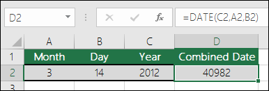
For example: =DATE(C2,A2,B2) combines the year from cell C2, the month from cell A2, and the day from cell B2 and puts them into one cell as a date. The example below shows the final result in cell D2.

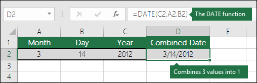
Need to insert dates without a formula? No problem. You can insert the current date and time in a cell, or you can insert a date that gets updated. You can also fill data automatically in worksheet cells.

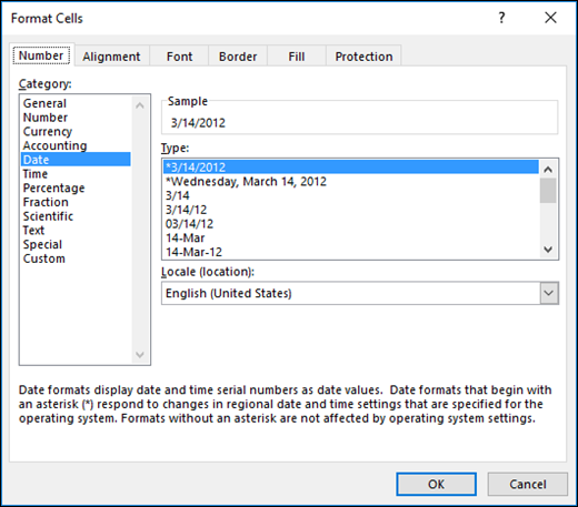
Right-click the cell(s) you want to change. On a Mac, Ctrl-click the cells.

On the Home tab click Format > Format Cells or press Ctrl+1 (Command+1 on a Mac).

3. Choose the Locale (location) and Date format you want.

For more information on formatting dates, see Format a date the way you want.

You can use the DATE function to create a date that is based on another cell’s date. For example, you can use the YEAR, MONTH, and DAY functions to create an anniversary date that’s based on another cell. Let’s say an employee’s first day at work is 10/1/2016; the DATE function can be used to establish his fifth year anniversary date:

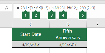
The DATE function creates a date.

The YEAR function looks at cell C2 and extracts «2012».

Then, «+5» adds 5 years, and establishes «2017» as the anniversary year in cell D2.

The MONTH function extracts the «3» from C2. This establishes «3» as the month in cell D2.

The DAY function extracts «14» from C2. This establishes «14» as the day in cell D2.

If you open a file that came from another program, Excel will try to recognize dates within the data. But sometimes the dates aren’t recognizable. This is may be because the numbers don’t resemble a typical date, or because the data is formatted as text. If this is the case, you can use the DATE function to convert the information into dates. For example, in the following illustration, cell C2 contains a date that is in the format: YYYYMMDD. It is also formatted as text. To convert it into a date, the DATE function was used in conjunction with the LEFT, MID, and RIGHT functions.

The DATE function creates a date.

The LEFT function looks at cell C2 and takes the first 4 characters from the left. This establishes “2014” as the year of the converted date in cell D2.

The MID function looks at cell C2. It starts at the 5th character, and then takes 2 characters to the right. This establishes “03” as the month of the converted date in cell D2. Because the formatting of D2 set to Date, the “0” isn’t included in the final result.

The RIGHT function looks at cell C2 and takes the first 2 characters starting from the very right and moving left. This establishes “14” as the day of the date in D2.

To increase or decrease a date by a certain number of days, simply add or subtract the number of days to the value or cell reference containing the date.

In the example below, cell A5 contains the date that we want to increase and decrease by 7 days (the value in C5).

Источник

The MONTH function in Excel is a date function used to find the month for a given date in a date format. This function takes an argument in a date format, and the result is in integer format. This function’s value is in the range of 1-12 as there are only twelve months in a year. The method to use this function is as follows =MONTH( serial_number). The argument provided to this function should be in a recognizable date format of Excel.

For example, =MONTH(A1) – returns the month of a date in A1.

=MONTH(DATE(2020,6,10)) – returns 6 corresponding to June.

Also, =MONTH(“10-June-2020”) – returns number 6 too.

The MONTH function in Excel gives the month from its date. It returns the month number ranging from 1 to 12.

MONTH Formula in Excel

Below is the MONTH Formula in Excel.

Or

MONTH( date )

MONTH in Excel – Illustration

Suppose a date (10 August, 18) is given in cell B3. You want to find the month in Excel of the given date in numbers.

You can use the MONTH formula in Excel given below:

= MONTH (B3)

Press the “Enter” key. The MONTH function in Excel will return 8.

You can also use the following MONTH formula in Excel:

= MONTH (“10 Aug 2018”)

Press the “Enter” key. The MONTH function will also return the same value.

The date 10 Aug 2018 refers to a value 43322 in Excel. You can also use this value directly as input to the MONTH function. The MONTH formula in Excel would be:

= MONTH (43322)

MONTH function in Excel will return 8.

Alternatively, you can also use the date in another format:

= MONTH (“10-Aug-2018”)

Excel MONTH function will also return 8.

Let us look at examples of where and how to use the MONTH function in Excel in various scenarios.

How to Use MONTH Function in Excel?

The MONTH function in Excel is very simple and easy to use. Let us understand the working of a MONTH in excel by some examples.

serial_number: a valid date for which the month number is to be identified

The input date must be a valid Excel dateThe date function in excel is a date and time function representing the number provided as arguments in a date and time code. The result displayed is in date format, but the arguments are supplied as integers.read more. The dates in Excel are stored as serial numbers. For example, the date Jan 1, 2010, equals the serial number 40179 in Excel. The MONTH formula in Excel takes as input both the date directly or the serial number of the date. It is to be noted here that Excel does not recognize dates earlier than 1/1/1900.

Returns

The MONTH function in Excel always returns a number ranging from 1 to 12. This number corresponds to the month of the input date.

You can download this MONTH Function Excel Template here – MONTH Function Excel Template

MONTH in Excel Example #1

Suppose you have a list of dates given in the cells B3: B7, as shown below. You want to find the month name of each of these given dates.

You can do so using the following MONTH formula in Excel:

= CHOOSE ((MONTH(B3)), “Jan”, “Feb”, “Mar”, “Apr”, “May”, “Jun”, “Jul”, “Aug”, “Sep”, “Oct”, “Nov”, “Dec”)

MONTH (B3) will return 1.

CHOOSE (1, …..) will choose the 1^st option of the given 12, Jan here.

So, the MONTH function in Excel will return Jan as a result.

Similarly, you can drag it for the rest of the cells.

Alternatively, you can use the following MONTH formula in Excel:

= TEXT (B3, “mmm”)

The MONTH function will return Jan as a result.

MONTH in Excel Example #2

Suppose you have month names (say in “mmm” format) given in cells B4: B15.

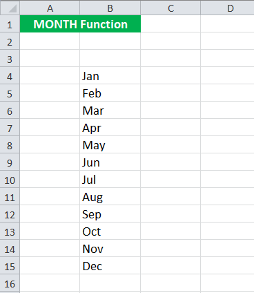
Now, you want to convert these names to the month in numbers.

You can use the following MONTH in Excel:

= MONTH ( DATEVALUE( B4 & ” 1”)

For Jan, the MONTH in Excel will return 1. For Feb, it will return 2 and so on.

MONTH in Excel Example #3

Suppose you have a list of holidays given in cells B3: B9 in a date-wise manner, as shown below.

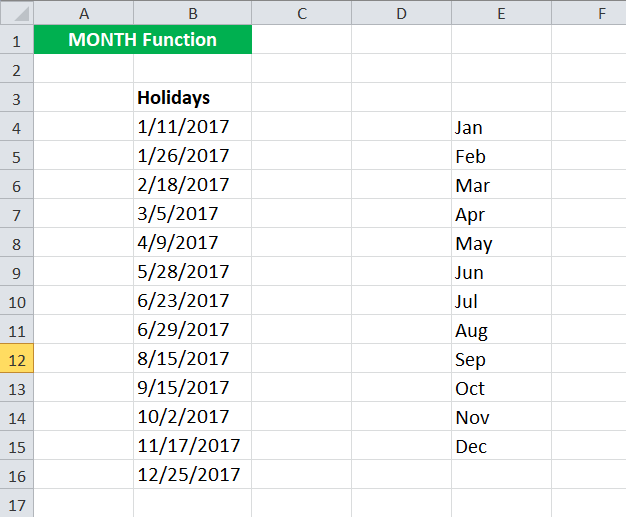
Now, you want to calculate the number of holidays each month. To do so, you can use the following MONTH formula in Excel for the first month given in E4:

= SUMPRODUCT( –( MONTH( $B$4:$B$16 ) = MONTH( DATEVALUE( E4 & ” 1″)) ) )

Then, drag it to the rest of the cells.

Let us look at the MONTH function in Excel detail:

• MONTH( $B$4:$B$16 ) will check the month of the dates provided in cell range B4:B16 in a number format. The MONTH function in Excel will return {1; 1; 2; 3; 4; 5; 6; 6; 8; 9; 10; 11; 12}
• MONTH( DATEVALUE( E4 & ” 1″) will give the month in number corresponding to cell E4 (see example 2). The MONTH function in Excel will return 1 for January
• SUMPRODUCT in ExcelThe SUMPRODUCT excel function multiplies the numbers of two or more arrays and sums up the resulting products.read more (– (…) = (..) ) will match the month given in B4:B16 with January (=1) and will add one each time when it is true.

Since January appears twice in the given data, the MONTH function in Excel will return 2.

Similarly, you can do for the rest of the cells.

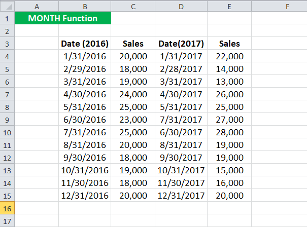
MONTH in Excel Example #4

Suppose you have sales data for the past two years. The data was collected on the last date of the month. The data was manually entered, so there could be a mismatch in the data. You should compare the sales between 2016 and 2017 for each month.

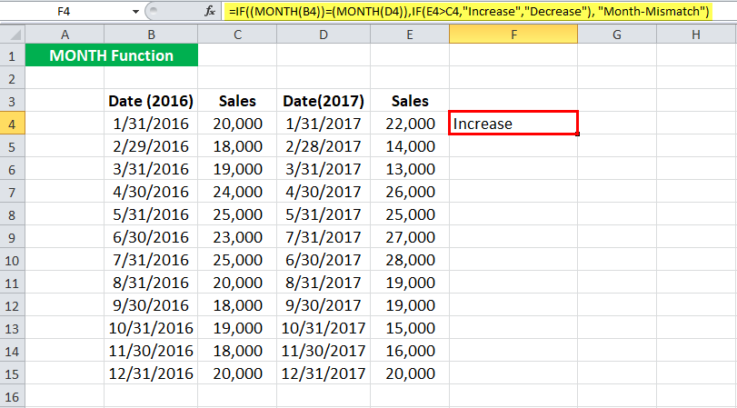
To check if the months are the same and then compare the sales, you can use the MONTH formula in Excel:

=IF( (MONTH(B4)) = (MONTH(D4) ), IF( E4 > C4, “Increase”, “Decrease” ),  “Month-Mismatch” )

For the first entry, the MONTH function in Excel will return “Increase.”

Let us look at the MONTH in Excel in detail:

If the MONTH of B4 (for 2016) is equal to the MONTH given in D4 (for 2017),

• The MONTH function in Excel will check if the sales for the given month in 2017 are greater than that in 2016.
  • If it is greater, it will return “Increase.”
  • Else, it will return to “Decrease.”

If the MONTH of B4 (for 2016) is not equal to the MONTH given in D4 (for 2017),

• The MONTH function in Excel will return “Mismatch.”

Similarly, you can do for the rest of the cells.

You could also add another condition to check if the sales are equal and return “Constant.”

MONTH in Excel Example #5

Suppose you work in your company’s sales department and have date-wise data of how many products were sold on a particular date for the previous year, as shown below.

Now, you want to club the number of products monthly. To do so, you use the following MONTH formula in Excel:

= SUMPRODUCT(– ( EXACT( F4, MONTH( $B$4:$B$17 ))), $C$4:$C$17 )

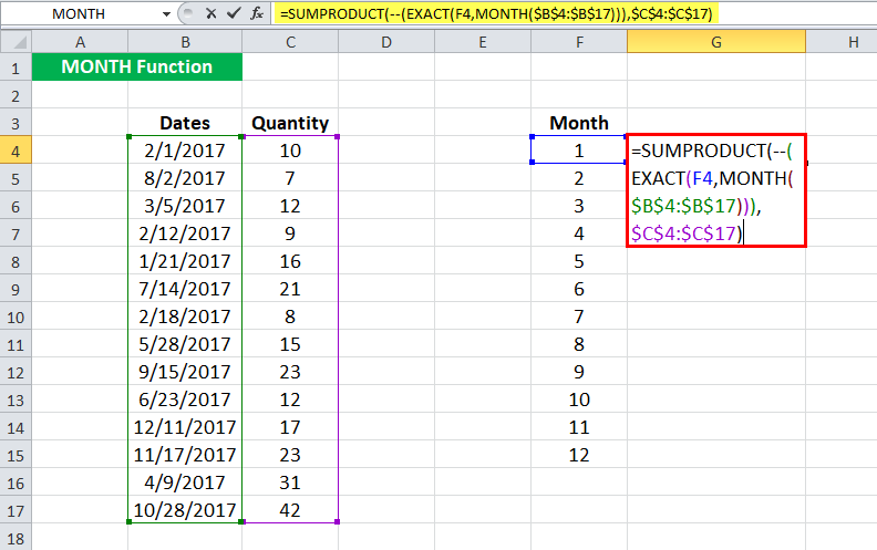
For the first cell, the MONTH function in Excel will return 16.

Then, drag it to the rest of the cells.

Let us look at the MONTH in Excel in detail:

= SUMPRODUCT(– ( EXACT( F4, MONTH( $B$4:$B$17 ))), $C$4:$C$17 )

• MONTH( $B$4:$B$17 ) will give the month of the cells in B4: B17. MONTH function in Excel will return a matrix {2; 8; 3; 2; 1; 7; 2; 5; 9; 6; 12; 11; 4; 10}
• EXACT( F4, MONTH( $B$4:$B$17 )) will match the month in F4 ( 1 here) with the matrix and will return another matrix with TRUE when it is a match or FALSE otherwise. For the 1st month, it will return {FALSE; FALSE; FALSE; FALSE; TRUE; FALSE; FALSE; FALSE; FALSE; FALSE; FALSE; FALSE; FALSE; FALSE}
• SUMPRODUCT (– (..), $C$4:$C$17) will sum the values in C4:C17 when the corresponding value in the matrix is “TRUE.”

The MONTH function in Excel will return 16 for January.

Things to remember about a MONTH in Excel

• The MONTH function returns the month of the given date or serial number.
• Excel MONTH function is given #VALUE! Error when it cannot recognize the date.
• The Excel MONTH function accepts dates only after 1 Jan 1900. It will provide the #VALUE! Error when the input date is earlier than 1 Jan 1900.
• The MONTH function in Excel returns the month in number format only. Therefore, its output is always a number between 1 and 12.

MONTH Excel Function Video

Recommended Articles

This article is a guide to MONTH Function in Excel. We discuss the MONTH formula in Excel and how to use the MONTH function, along with Excel examples and downloadable Excel templates. You may also look at these useful functions in Excel: –

• EDATE Function in ExcelEDATE is a date and time function in excel which adds a given number of months into a date and gives us a date in a numerical format of date. It takes dates and integers as input, the output returned by this function is also a date value. read more
• VBA MONTH VBA Month Function is an inbuilt function that is used to extract the month from a date. The output of this function is an integer ranging from 1 to 12. Only the month number is extracted from the supplied date value by this function.read more
• EOMONTH in ExcelEOMONTH is a worksheet date function in excel which calculates the end of the month for the given date by adding a specified number of months to the arguments. This function takes two arguments: the date and another as integer, and the output is in the date format.read more
• FREQUENCY Excel FunctionThe FREQUENCY function in Excel calculates the number of times a data values occurs within a given range of values and returns a vertical array of numbers corresponding to each value’s frequency within a range.read more