What is mirr in excel - Word и Excel - помощь в работе с программами

Excel for Microsoft 365 Excel for Microsoft 365 for Mac Excel for the web Excel 2021 Excel 2021 for Mac Excel 2019 Excel 2019 for Mac Excel 2016 Excel 2016 for Mac Excel 2013 Excel 2010 Excel 2007 Excel for Mac 2011 Excel Starter 2010 More…Less

This article describes the formula syntax and usage of the MIRR function in Microsoft Excel.

Description

Returns the modified internal rate of return for a series of periodic cash flows. MIRR considers both the cost of the investment and the interest received on reinvestment of cash.

Syntax

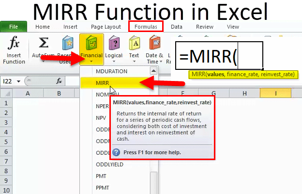
MIRR(values, finance_rate, reinvest_rate)

The MIRR function syntax has the following arguments:

Values Required. An array or a reference to cells that contain numbers. These numbers represent a series of payments (negative values) and income (positive values) occurring at regular periods.
- Values must contain at least one positive value and one negative value to calculate the modified internal rate of return. Otherwise, MIRR returns the #DIV/0! error value.
- If an array or reference argument contains text, logical values, or empty cells, those values are ignored; however, cells with the value zero are included.
Finance_rate Required. The interest rate you pay on the money used in the cash flows.
Reinvest_rate Required. The interest rate you receive on the cash flows as you reinvest them.

Remarks

MIRR uses the order of values to interpret the order of cash flows. Be sure to enter your payment and income values in the sequence you want and with the correct signs (positive values for cash received, negative values for cash paid).
If n is the number of cash flows in values, frate is the finance_rate, and rrate is the reinvest_rate, then the formula for MIRR is:

Example

Copy the example data in the following table, and paste it in cell A1 of a new Excel worksheet. For formulas to show results, select them, press F2, and then press Enter. If you need to, you can adjust the column widths to see all the data.

Data	Description
-120000	Initial cost
39000	Return first year
30000	Return second year
21000	Return third year
37000	Return fourth year
46000	Return fifth year
0.1	Annual interest rate for the 120,000 loan
0.12	Annual interest rate for the reinvested profits
Formula	Description	Result
=MIRR(A2:A7, A8, A9)	Investment’s modified rate of return after five years	13%
=MIRR(A2:A5, A8, A9)	Modified rate of return after three years	-5%
=MIRR(A2:A7, A8, 14%)	Five-year modified rate of return based on a reinvest_rate of 14 percent	13%

Need more help?

Источник

Modified Internal Rate of Return

What is MIRR?

The Modified Internal Rate of Return (MIRR)[1] is a function in Excel that takes into account the financing cost (cost of capital) and a reinvestment rate for cash flows from a project or company over the investment’s time horizon.

The standard Internal Rate of Return (IRR) assumes that all cash flows received from an investment are reinvested at the same rate. The Modified Internal Rate of Return (MIRR) allows you to set a different reinvestment rate for cash flows received. Additionally, MIRR arrives at a single solution for any series of cash flows, while IRR can have two solutions for a series of cash flows that alternate between negative and positive.

To learn more, launch our Advanced Excel Formulas course now!

What is the Modified Internal Rate of Return (MIRR) Formula in Excel?

The MIRR formula in Excel is as follows:

=MIRR(cash flows, financing rate, reinvestment rate)

Where:

Cash Flows – Individual cash flows from each period in the series
Financing Rate – Cost of borrowing or interest expense in the event of negative cash flows
Reinvestment Rate – Compounding rate of return at which positive cash flow is reinvested

An Example of the Modified Internal Rate of Return

Below is an example that provides the most clear-cut example of how MIRR differs from standard IRR.

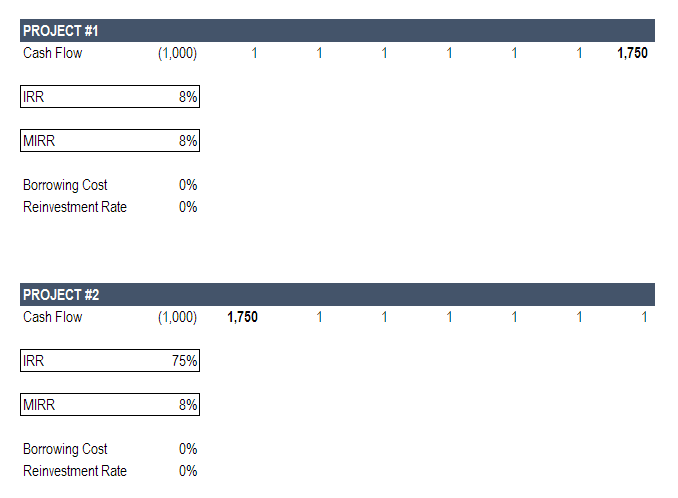
In the example below, we imagine two different projects. In both cases the total amount of cash received over the investment’s life is the same – the only difference is the timing of those cash flows.

Here are the key assumptions:

Initial investment: $1,000 (same in both projects)
Major positive cash flow: $1,750 (same in both cases)
Timing of major cash flow: last year in Project 1; first year in Project 2
Reinvestment rate for MIRR: 0%

To learn more, launch our Advanced Excel Formulas course now!

As you can see in the image above, there is a major difference in the return calculated by MIRR and IRR in Project #2. In project #1, there is no difference.

Let’s break down the reasons why.

MIRR Project #1

In Project #1, essentially all cash flow is received at the end of the project, so the reinvestment rate is irrelevant.

It’s important to show this case to clearly illustrate that reinvestment doesn’t matter when a project only has one final cash flow. Examples would be a zero-coupon bond or a Leveraged Buyout (LBO) where all cash flow is used to service debt until the company is sold for one large lump sum.

MIRR Project #2

In Project #2, by contrast, essentially all of the cash flow is received in year one. This means that the reinvestment rate is going to play a big role in the overall IRR of the project.

Since we set the reinvestment rate for MIRR to 0%, we can make an extreme example to illustrate the point.

The life of the investment is 7 years, so let’s look at what each result is saying.

MIRR is saying that, if you invested $1,000 at 8% for 7 years you would have $1,756 by the end of the project. If you sum up the cash flows in the example, you get $1,756, so this is correct.

So, why is the IRR result of 75% saying? Clearly, it’s not saying that if you invested $1,000 at 8% for 7 years you would have $50,524.

Recall that IRR is the discount rate that sets the Net Present Value (NPV) of an investment to zero. So, what the IRR case is saying is simply that discounting the $1,750 cash flow in year one needs to be discounted by 75% to arrive at an NPV of $0.

Which is Better, IRR or MIRR?

The answer is that it depends on what you’re trying to show and what the takeaway is. It can be helpful to look at both cases and play with different reinvestment rates in the MIRR scenario.

One thing that can be definitively said is that MIRR offers more control and is more precise.

To learn more, launch our Advanced Excel Formulas course now!

MIRR Application in Financial Modeling

When it comes to financial modeling, and specifically in private equity and investment banking, the standard IRR function is common practice. The reason for this is that transactions are looked at in isolation and not with the effect of then another investment assumption layered in.

MIRR requires an additional assumption, which could make two different transactions less comparable.

To master the art of building a financial model, launch our financial modeling courses now!

The Downside of Using Modified Internal Rate of Return

There are some downsides to using MIRR, the main one being the added complexity of making additional assumptions about what rate funds will be reinvested at. Additionally, it is not nearly as widely used as traditional IRR, so it will require more socializing, buy-in, and explaining at most corporations, banks, accounting firms, and institutions.

Additional Resources

We hope this has been a useful guide to the Modified Internal Rate of Return MIRR, how to use it in Excel, and what the pros and cons of it are.

For more learning and development, we highly recommend the following additional CFI resources:

XIRR vs IRR
XNPV vs NPV
Financial Modeling Guide
The Analyst Trifecta®
See all Excel resources

Article Sources

MIRR Function

Источник

SOLVED: How To Invert a Table In Excel (Swap The Columns and Rows)

In Excel, select all of the data you are interested in, right click.
select COPY.
Right click on an empty cell elsewhere in the same or a different worksheet.
Select PASTE SPECIAL > PASTE SPECIAL > click TRANSPOSE > click OK.

Contents

1 How do you invert a table?
2 Can you Transpose a whole table in Excel?
3 How do you invert and paste in Excel?
4 How do I invert a column in Excel?
5 How do you reshape data in Excel?
6 What is the slicer?
7 How do I mirror text in Excel?
8 How do you reverse a string in Excel?
9 How do you reverse the order of data in Excel?
10 What does Alt DP do in Excel?
11 How do you use concatenate?
12 How do you transform data from long to wide in Excel?
13 How do you make Excel Slicers look like tabs?
14 Can we use slicer without pivot table?
15 Is there a mirror function in Excel?
16 How do you invert text?
17 How do I make a cell mirror in Excel?
18 How do you make a clustered bar chart in Excel?

Select an empty cell below your pasted table. Click the arrow under the “Paste” button on the ribbon and choose the “Transpose” option. Your table will appear flipped.

Can you Transpose a whole table in Excel?

Start by selecting and copying your entire data range. Click on a new location in your sheet, then go to Edit | Paste Special and select the Transpose check box, as shown in Figure B. Click OK, and Excel will transpose the column and row labels and data, as shown in Figure C.

How do you invert and paste in Excel?

How to copy and paste data in reverse order in Excel?

In an empty column, put in the number 1 for the first.
Drag 1 down to create a list of numbers in increasing order (press Cntrl and drag down)
Turn on the auto filter for the list of data to be reversed.

How do I invert a column in Excel?

Flip a column of data order in Excel with Sort command

Insert a series of sequence numbers besides the column.
Click the Data > Sort Z to A, see screenshot:
In the Sort Warning dialog box, check the Expand the selection option, and click the Sort button.
Then you will see the number order of Column A is flipped.

How do you reshape data in Excel?

Open your Excel file and go to “Data Tool” tab. Mark your data and click on “Reshape 1Dim” or “Reshape 2Dim”, based on the format of your data. If your data is in one column so click on “Reshape 1Dim” otherwise click on “Reshape 2Dim”.

What is the slicer?

Slicers provide buttons that you can click to filter tables, or PivotTables. In addition to quick filtering, slicers also indicate the current filtering state, which makes it easy to understand what exactly is currently displayed. WindowsmacOSWeb. You can use a slicer to filter data in a table or PivotTable with ease.

How do I mirror text in Excel?

Reverse or mirror text

Insert a text box in your document by clicking Insert > Text Box, and then type and format your text. For more details, see Add, copy, or delete a text box.
Right-click the box and click Format Shape.
In the Format Shape pane, click Effects.
Under 3-D Rotation, in the X Rotation box, enter 180.

How do you reverse a string in Excel?

Reverse a Text String in Excel using TRANSPOSE Formula
In cell B1, type the formula: =TRANSPOSE(MID(A1,LEN(A1)-ROW(INDIRECT(“1:”&LEN(A1)))+1,1)) in cell B1. Select the entire formula in the formula bar and press F9 on your keyboard. This should display each character of your string, reversed and separated by commas.

How do you reverse the order of data in Excel?

Begin by highlighting those cells. Click on Data in the toolbar and then on Sort , producing the screenshot at left. To reverse the order, click on Descending and then on OK .

What does Alt DP do in Excel?

If you sequentially press ALT, D and P on the keyboard, Excel will open to create a pivot table wizard. Select the appropriate option. The selected option in the above screenshot will lead us to create a pivot table as we created before.

How do you use concatenate?

There are two ways to do this:

Add double quotation marks with a space between them ” “. For example: =CONCATENATE(“Hello”, ” “, “World!”).
Add a space after the Text argument. For example: =CONCATENATE(“Hello “, “World!”). The string “Hello ” has an extra space added.

How do you transform data from long to wide in Excel?

Suppose you have data that is stored in long format in excel. You want to reshape it to wide format. Press CTRL + SHIFT + ENTER to confirm this formula as it’s an array formula.

How do you make Excel Slicers look like tabs?

To do so, select the chart. Click the contextual Format tab and choose a color from the Shape Outline dropdown. The slicer buttons look like tabs, as we saw in Figure B.

Can we use slicer without pivot table?

The chart data and the values in G1:G13 will change based on the selected Cost Center from the slicers list as can be seen the data in the range B1:F13 can be filtered with a slicer without inserting a Pivot Table.

Is there a mirror function in Excel?

Mirror/link cells across worksheets with From Microsoft Query feature. This method will walk you through mirroring table of another workbook with the From Microsoft Query feature in Excel. 2. In the Choose Data Source dialog box, select the Excel Files* in the left box, and click the OK button.

How do you invert text?

Use a text box

Right-click the text box and choose Format Shape.
Choose 3-D Rotation in the left pane.
Change the X setting to 180.
Click OK, and Word flips the text in the text box, producing a mirror image. You can create an upside-down mirror image by changing the Y setting to 180.

How do I make a cell mirror in Excel?

If you want the contents of, say, C1 to mirror the contents of cell A1, you just need to set the formula in C1 to =A1 . From this point forward, anything you type in A1 will show up in C1 as well. Well the simplest way is to have a formula in Z99 =B4 so that when you type in B4 Excel will copy the value to Z99.

How do you make a clustered bar chart in Excel?

How to Make a Clustered Bar chart in Excel

Step 1: Select the data you want displayed in the Clustered Bar chart.
Step 2: Click the Insert Tab, and then Click the Bar Symbol in the Charts Group.
Step 3: Click the Clustered Bar button from the Insert Column or Bar Chart window.

Источник

Contents

1 What is MIRR formula?
2 What does MIRR means in Excel?
3 How do you do MIRR on a calculator?
4 What is the MIRR rule?
5 How do you calculate MIRR on a TI 84?
6 Is MIRR lower than IRR?
7 Is MIRR better than IRR?
8 How do you use Marr?
9 How do you calculate Mirr reinvestment?
10 What is MIRR in simple terms?
11 Which is better NPV or MIRR?
12 What is cost of capital in MIRR?
13 Is WACC same as IRR?
14 How is IRR calculated in insurance?
15 Is WACC same as discount rate?
16 How do we calculate payback period?
17 How do you find the discounted payback period?
18 What is Xirr and MIRR?
19 What is IRR and Marr?
20 How do you clear CF on a financial calculator?

What is MIRR formula?

The Formula for MIRR is: MIRR = (Terminal Cash inflows/ PV of cash out flows) ^ⁿ – 1. n = the number of years for the project. Terminal Value= future value of cash inflows to be reinvested in the project at the cost of capital.

What does MIRR means in Excel?

modified internal rate of return
Description. Returns the modified internal rate of return for a series of periodic cash flows. MIRR considers both the cost of the investment and the interest received on reinvestment of cash.

How do you do MIRR on a calculator?

Press “I/YR” to solve for the percentage rate of return that grows the cost of the investment to the future value of the reinvested cash flows, which is the MIRR.

What is the MIRR rule?

MIRR calculates the return on investment based on the more prudent assumption that the cash inflows from a project shall be re-invested at the rate of the cost of capital.The decision rule for MIRR is very similar to IRR, i.e. an investment should be accepted if the MIRR is greater than the cost of capital.

How do you calculate MIRR on a TI 84?

How to Calculate MIRR on TI 84 Plus

Bring up the TMV Solver app by pressing APPS, ENTER, ENTER.
Enter the following: N = 2; I% = 0.12, PV = -1.95, PMT = 0, FV = 2.6652; P/Y =1; C/Y = END.
Press APPS, ENTER, 7, which brings up NPV on the screen.
Enter the NPV cash flow information as NPV (12, -1.95, {1.21, 1.31}) ENTER.

Is MIRR lower than IRR?

MIRR is invariably lower than IRR and some would argue that it makes a more realistic assumption about the reinvestment rate. However, there is much confusion about what the reinvestment rate implies. Both the NPV and the IRR techniques assume the cash flows generated by a project are reinvested within the project.

Is MIRR better than IRR?

The decision criterion of both the capital budgeting methods is same, but MIRR delineates better profit as compared to the IRR, because of two major reasons, i.e. firstly, reinvestment of the cash flows at the cost of capital is practically possible, and secondly, multiple rates of return don’t exist in the case of

How do you use Marr?

The formula for MARR is: MARR = project value + rate of interest for loans + expected rate of inflation + rate of inflation change + loan default risk + project risk.
The formula for current return is: current return = (the present value of cash inflows + the present value of cash outflows) / interest rate.

How do you calculate Mirr reinvestment?

The reinvestment approach assumes cash flows are reinvested at the firm’s cost of capital: $150 (cash flow at year one) * 1.14 = $171 + $200 (cash flow at year two) = $371 $371 = future value of positive cash flow at the second year. The MIRR equals 21.81%.

What is MIRR in simple terms?

The modified internal rate of return (MIRR) assumes that positive cash flows are reinvested at the firm’s cost of capital and that the initial outlays are financed at the firm’s financing cost.The MIRR, therefore, more accurately reflects the cost and profitability of a project.

Which is better NPV or MIRR?

When the investment and reinvestment rates are the same as the NPV discount rate, MIRR is the equivalent of the NPV in percentage terms. When they are different, MIRR will be the better measure because it directly accounts for reinvestment of the cash flows at the different rate.

What is cost of capital in MIRR?

The Modified Internal Rate of Return (MIRR) is a function in Excel that takes into account the financing cost (cost of capital) and a reinvestment rate for cash flows.In other words, it is the expected compound annual rate of return that will be earned on a project or investment.

Is WACC same as IRR?

IRR & WACC
The primary difference between WACC and IRR is that where WACC is the expected average future costs of funds (from both debt and equity sources), IRR is an investment analysis technique used by companies to decide if a project should be undertaken.

How is IRR calculated in insurance?

Put =IRR in the last cell and select all the data of the column from the 1st premium value till the net cash inflow amount and then press enter. You will get the required IRR value and this is the return which you look for.
How to calculate returns from insurance?

Years	Premium
IRR	31.74 per cent

Is WACC same as discount rate?

The discount rate is the interest rate used to determine the present value of future cash flows in a discounted cash flow (DCF) analysis.Many companies calculate their weighted average cost of capital (WACC) and use it as their discount rate when budgeting for a new project.

How do we calculate payback period?

To calculate the payback period you can use the mathematical formula: Payback Period = Initial investment / Cash flow per year For example, you have invested Rs 1,00,000 with an annual payback of Rs 20,000. Payback Period = 1,00,000/20,000 = 5 years.

How do you find the discounted payback period?

The discounted payback period is calculated by discounting the net cash flows of each and every period and cumulating the discounted cash flows until the amount of the initial investment is met.

What is Xirr and MIRR?

XIRR is the IRR when the periodicity between cash flows is not equal. XMIRR is the MIRR when periodicity between cash flows is not equal. Net Present Value (NPV) Net Present Value is the current value of a future series of payments and receipts and a way to measure the time value of money.

What is IRR and Marr?

The IRR is a measure of the percentage yield on investment. The IRR is corn- pared against the investor’s minimum acceptable rate of return (MARR), to ascertain the economic attractiveness of the investment.If the IRR equals the MARR, the investment’s benefits or sav- ings just equal its costs.

How do you clear CF on a financial calculator?

Using the Cash Flow Feature on Your Financial Calculator. Clear the Cash Flow Memory by pushing CF, 2^nd and then the CE/C button.

Источник

Содержание

Функция МВСД
Синтаксис
Замечания
Пример
См. также
Поддержка и обратная связь
MIRR function
Description
Syntax
Remarks
Example
MIRR function
Description
Syntax
Remarks
Example
Функция MIRR
Пример
Метод WorksheetFunction.MIrr (Excel)
Синтаксис
Параметры
Возвращаемое значение
Замечания
Поддержка и обратная связь

Функция МВСД

Возвращает значение типа Double, определяющее измененную внутреннюю норму прибыли для последовательности периодических потоков денежных средств (платежи и поступления).

Синтаксис

MIRR(values( ), finance_rate, reinvest_rate)

Функция MIRR использует следующие именованные аргументы:

Part	Описание
values( )	Обязательно. Массив с типом Double, определяющий значения денежного потока. Этот массив должен содержать по крайней мере одно отрицательное значение (платеж) и одно положительное значение (получение).
finance_rate	Обязательно. Значение типа Double, определяющее процентную ставку, представляющую собой стоимость финансирования.
reinvest_rate	Обязательно. Значение типа Double, определяющее процентную ставку прибыли, получаемую благодаря реинвестированию денежных средств.

Замечания

Измененная внутренняя норма прибыли — это внутренняя норма прибыли для случая, когда для финансирования платежей и поступлений используются различные ставки. Функция MIRR учитывает как стоимость инвестиций (finance_rate), так и процентную ставку, получаемую от реинвестирования денежных средств (reinvest_rate).

Аргументыfinance_rate и reinvest_rate — это проценты, выраженные в виде десятичных значений. Например, 12 процентов представляется как 0,12.

Функция MIRR использует порядок значений в массиве для интерпретации порядка платежей и поступлений. Следите, чтобы значения платежей и поступлений указывались в правильном порядке.

Пример

В этом примере функция MIRR используется для возврата измененной внутренней нормы доходности для ряда денежных потоков, содержащихся в массиве Values() . LoanAPR представляет проценты по финансированию и InvAPR процентную ставку, полученную при реинвестировании.

См. также

Поддержка и обратная связь

Есть вопросы или отзывы, касающиеся Office VBA или этой статьи? Руководство по другим способам получения поддержки и отправки отзывов см. в статье Поддержка Office VBA и обратная связь.

Источник

MIRR function

This article describes the formula syntax and usage of the MIRR function in Microsoft Excel.

Description

Returns the modified internal rate of return for a series of periodic cash flows. MIRR considers both the cost of the investment and the interest received on reinvestment of cash.

Syntax

MIRR(values, finance_rate, reinvest_rate)

The MIRR function syntax has the following arguments:

Values Required. An array or a reference to cells that contain numbers. These numbers represent a series of payments (negative values) and income (positive values) occurring at regular periods.

Values must contain at least one positive value and one negative value to calculate the modified internal rate of return. Otherwise, MIRR returns the #DIV/0! error value.

If an array or reference argument contains text, logical values, or empty cells, those values are ignored; however, cells with the value zero are included.

Finance_rate Required. The interest rate you pay on the money used in the cash flows.

Reinvest_rate Required. The interest rate you receive on the cash flows as you reinvest them.

MIRR uses the order of values to interpret the order of cash flows. Be sure to enter your payment and income values in the sequence you want and with the correct signs (positive values for cash received, negative values for cash paid).

If n is the number of cash flows in values, frate is the finance_rate, and rrate is the reinvest_rate, then the formula for MIRR is:

Example

Источник

MIRR function

This article describes the formula syntax and usage of the MIRR function in Microsoft Excel.

Description

Returns the modified internal rate of return for a series of periodic cash flows. MIRR considers both the cost of the investment and the interest received on reinvestment of cash.

Syntax

MIRR(values, finance_rate, reinvest_rate)

The MIRR function syntax has the following arguments:

Values Required. An array or a reference to cells that contain numbers. These numbers represent a series of payments (negative values) and income (positive values) occurring at regular periods.

Values must contain at least one positive value and one negative value to calculate the modified internal rate of return. Otherwise, MIRR returns the #DIV/0! error value.

If an array or reference argument contains text, logical values, or empty cells, those values are ignored; however, cells with the value zero are included.

Finance_rate Required. The interest rate you pay on the money used in the cash flows.

Reinvest_rate Required. The interest rate you receive on the cash flows as you reinvest them.

If n is the number of cash flows in values, frate is the finance_rate, and rrate is the reinvest_rate, then the formula for MIRR is:

Example

Источник

Функция MIRR

Возвращает значение типа Double, определяющее измененную внутреннюю норму прибыли для циклических потоков денежных средств (выплат и поступлений).

Функция MIRR имеет следующие аргументы:

Обязательный аргумент. Массив типа double, состоящий из значений движений денежных средств. Массив должен содержать по крайней мере одно отрицательное значение (выплата) и одно положительное значение (поступление).

Обязательный аргумент. Значение типа Double, обозначающее процентную ставку платежей по инвестированию средств.

Обязательный аргумент. Значение типа Double, обозначающее процентную ставку дохода от инвестирования средств.

Измененной внутренней нормой прибыли называется внутренняя норма прибыли в том случае, когда платежи и поступления финансовых средств осуществлялись по разным процентным ставкам. При выполнении функции MIRR учитываются как затраты на инвестиции ( ставка_финанс), так и доход, полученный от инвестирования ( ставка_реинвест).

Аргументы ставка_финанс и ставка_реинвест являются процентными значениями, выраженными как десятичные числа. Например, значение «12 процентов» задается как 0,12.

Функция MIRR определяет порядок выплат и поступлений на основе порядка значений в массиве. Убедитесь, что значения выплат и поступлений указаны в правильном порядке.

Пример

Примечание: В примерах ниже показано, как использовать эту функцию в модуле Visual Basic для приложений (VBA). Чтобы получить дополнительные сведения о работе с VBA, выберите Справочник разработчика в раскрывающемся списке рядом с полем Поиск и введите одно или несколько слов в поле поиска.

В этом примере с помощью функции MIRR возвращается измененная внутренняя норма прибыли для последовательности денежных потоков, заданной массивом Values() . Переменная LoanAPR отражает ставку финансирования, а переменная InvAPR — ставку доходности инвестиций.

Источник

Метод WorksheetFunction.MIrr (Excel)

Возвращает измененную внутреннюю норму прибыли для ряда периодических денежных потоков. MIrr учитывает как стоимость инвестиций, так и проценты, полученные на реинвестирование денежных средств.

Синтаксис

expression. MIrr (Arg1, Arg2, Arg3)

Выражение Переменная, представляющая объект WorksheetFunction .

Параметры

Имя	Обязательный или необязательный	Тип данных	Описание
Arg1	Обязательный	Variant	Значения — массив или ссылка на ячейки, содержащие числа. Эти числа представляют собой ряд платежей (отрицательные значения) и доходов (положительные значения), происходящих в регулярные периоды.
Arg2	Обязательный	Double	Finance_rate — процентная ставка, которую вы платите на деньги, используемые в денежных потоках.
Arg3	Обязательный	Double	Reinvest_rate — процентная ставка, которую вы получаете на денежные потоки при их реинвесте.

Возвращаемое значение

Double

Замечания

Значения должны содержать по крайней мере одно положительное и одно отрицательное значение для вычисления измененной внутренней скорости возврата; В противном случае MIrr возвращает #DIV/0! значение ошибки.

Если массив или ссылочный аргумент содержит текст, логические значения или пустые ячейки, эти значения игнорируются; однако включаются ячейки с нулевым значением.

MIrr использует порядок значений для интерпретации порядка денежных потоков. Обязательно введите значения платежей и доходов в нужной последовательности и с правильными знаками (положительные значения для полученных денежных средств, отрицательные значения для выплаченных денежных средств).

Если n — это количество денежных потоков в значениях, frate — finance_rate, а rrate — это reinvest_rate, формула MIrr :

Поддержка и обратная связь

Источник

MIRR in Excel (Table of Contents)

MIRR in Excel
MIRR Formula in Excel
How to Use MIRR Function in Excel?

MIRR in Excel

MIRR function under the financial category is a unique statistical function that provides the interest rate on invested amount and finds a series of net income against the invested amount. For using MIRR, we must have a series of investments, finance rate, and reinvest rate, and also argument should contain at least one positive and one negative value as well.

MIRR Formula in Excel

The Formula for the MIRR Function in Excel is as follows:

The MIRR function syntax or formula has the below-mentioned arguments:

Values: It is a cell reference or array which refers to the schedule of cash flows, including the initial investment with a negative sign at the start of the stream

Note: The array must contain at least one negative value (initial payment) and one positive value (returns). Here negative values are considered as payments, whereas Positive values are treated as income.

Finance_rate: It’s a cost of borrowing or interest rate paid on the money used in the cash flows (negative cash flow)

Note: It can also be entered as a decimal value, i.e. 0.07 for 7%

Reinvest_rate: It’s an interest rate that you receive on the reinvested cash flow amount (Positive cash flow)

Note: It can also be entered as a decimal value, i.e. 0.07 for 7%

MIRR FUNCTION helps out in separating out negative & positive cash flows & discounting them at the appropriate rate.

How to Use MIRR Function in Excel

MIRR Function in Excel is very simple and easy to use. Let us understand the working of MIRR in Excel by Some Examples.

You can download this MIRR Function Excel Template here – MIRR Function Excel Template

Example #1

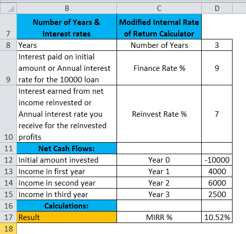
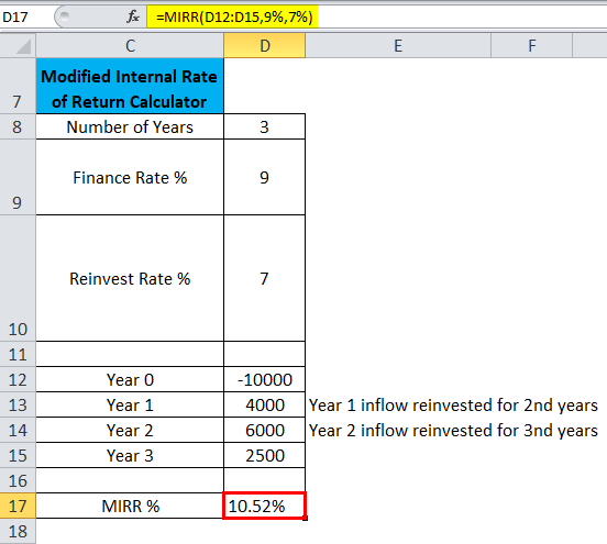
In the below-mentioned example, the Table contains the below-mentioned details.

Initial investment: 10000, Finance rate for MIRR is 9% & Reinvestment rate for MIRR is 7%

Positive cash flow: Year 1: 4000

Year 2: 6000

Year 3: 2500

I need to find out the investment’s Modified Internal Rate of Return (MIRR) after three years by using the MIRR Function.

Let’s apply the MIRR function in cell “D17”.

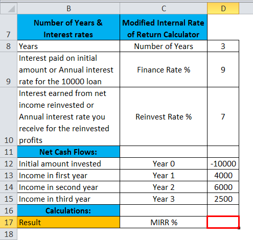
Select the cell “D17” where the MIRR function needs to be applied; click the insert function button (fx) under formula toolbar, a dialog box will appear, type the keyword “MIRR” in the search for a function box, MIRR function will appear in select a function box.

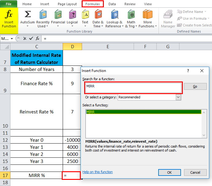
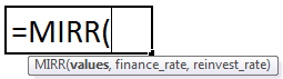
Double click on MIRR function, A dialog box appears where arguments for max function needs to be filled or entered, i.e. =MIRR(values, finance_rate, reinvest_rate

values argument: It is a cell reference or array which refers to the schedule of cash flows including the initial investment with a negative sign at the start of the stream. To select an array or cell reference, click inside cell D12 and you’ll see the cell selected, then Select the cells till D15. So that column range will get selected, i.e. D12:D15

finance_rate: It is the Interest paid on an initial amount or Annual interest rate for the 10000 loans, i.e. 9% or 0.09

reinvest_rate: Interest earned from net income reinvested or the Annual interest rate you receive for the reinvested profits, i.e. 7% or 0.07

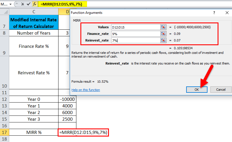
Click ok after entering the three arguments. =MIRR(D12:D15,9%,7%), i.e. returns the investment’s Modified Internal Rate of Return (MIRR) after three years. i.e. 10.52% in the cell D17

Note: Initially, it will return the value 11%, But to get a more precise value We have to click on increase decimal place by 2 points. So that it will give an exact investment’s returns, i.e. 10.52%

Example #2

In the below-mentioned table, Suppose I want to choose one project from two given projects with the same initial investment of 100000.

Here I need to compare the Five-year modified internal rate of returns based on a 9% finance rate & reinvest_rate of 7% percent for both the project with an initial investment of 100000.

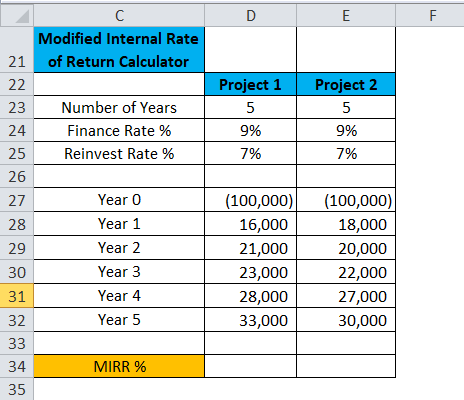
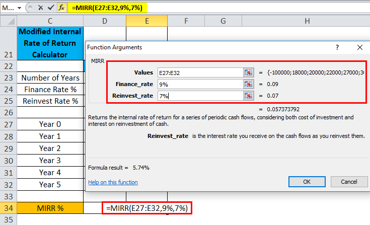
Let’s apply the MIRR function in cell “D34” for project 1 & “E34” for project 2.

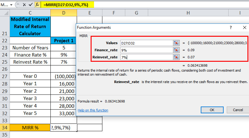
Select the cell “D34” where the MIRR function needs to be applied; click the insert function button (fx) under formula toolbar, a dialog box will appear, type the keyword “MIRR” in the search for a function box, MIRR function will appear in select a function box.

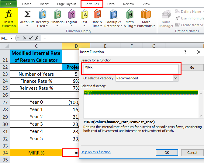
The above step is simultaneously applied in cell “E34.”

Double click on the MIRR function, A dialog box appears where arguments for max function needs to be filled or entered =MIRR(values, finance_rate, reinvest_rate) for project 1.

values argument: It is a cell reference or array which refers to the schedule of cash flows, including the initial investment with a negative sign at the start of the stream. To select an array or cell reference, click inside cell D27 and you’ll see the cell selected, then Select the cells till D32. So that column range will get selected, i.e. D27:D32

finance_rate: It is the Interest paid on an initial amount or Annual interest rate for the 10000 loans, i.e. 9% or 0.09

reinvest_rate: Interest earned from net income reinvested or the Annual interest rate you receive for the reinvested profits, i.e. 7% or 0.07

A similar procedure is followed for project 2 (Ref: Below mentioned screenshot)

Note: To get a more precise value, We have to click on increase decimal place by 2 points in cell D34 & E34 for both project 1 & 2 So that it will give an exact investment’s returns.

For project 1

=MIRR(D27:D32,9%,7%), i.e. returns the investment’s Modified Internal Rate of Return (MIRR) after three years. i.e. 6.34% in the cell D34

For project 2

=MIRR(E27:E32,9%,7%), i.e. returns the investment’s Modified Internal Rate of Return (MIRR) after three years. i.e. 5.74% in the cell E34

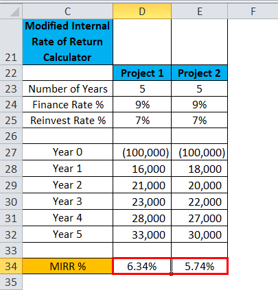
Inference: Based on the MIRR calculation, Project 1 is preferable; it has given better returns compared to project 2

Things to Remember

Values must contain at least one negative value & one positive value to calculate the modified internal rate of return. Otherwise, MIRR returns the #DIV/0! error
If an array or reference argument contains empty cells, text or logical values, those values are ignored
#VALUE! error occurs if any of the supplied arguments is not a numeric value or non-numeric
Initial investment needs to be in a negative value; otherwise, the MIRR Function will return an error value (#DIV/0! Error)
MIRR Function takes into consideration both the cost of the investment (finance_rate) and the interest rate received on cash reinvestment (reinvest_rate).
The main Difference between MIRR & IRR is MIRR considers the interest received on the reinvestment of cash, whereas the IRR does not consider it.

MIRR Function in Excel

The MIRR in Excel is a built-in financial function used to calculate the modified internal rate of return for the cash flows supplied with a period. This function takes the initial investment or loan values and a set of net income values with the interest rate paid on the initial amount, including the interest earned from reinvestment of earned amount, and returns the MIRR (Modified Internal Rate of Return) as output.

MIRR Function in Excel
- Syntax
- How to use the MIRR Function in Excel? (with Examples)
  - Example #1
  - Example #2
- Things to Remember
- Recommended Articles

Syntax

Parameters

The details of the parameters used in the MIRR formula in Excel are as follows:

Values: Values are an array of cash flow representing a series of payment amounts, range of references, or set of income values, including the initial investment amount.
Finance_rate: The finance rate is a rate of interest paid on the amount used during cash flow.
Reinvest_rate: Reinvest rate is the interest rate earned from the reinvested profit amount during cash flow.

How to use the MIRR Function in Excel? (with Examples)

You can download this MIRR Function Excel Template here – MIRR Function Excel Template

Example #1

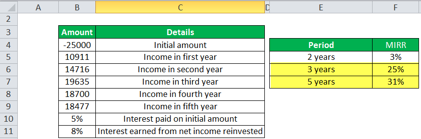
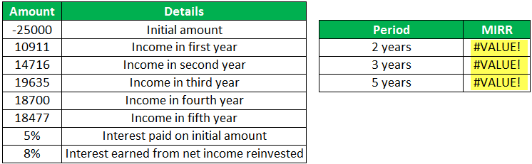
Consider an initial loan amount of 25,000 as an initial investment amount (loan amount) with an interest rate of 5% yearly. You have earned an interest rate of 8% from the reinvested income. In MIRR, the loan or initial investment amount is always considered as (-ve) value.

Below is the table that shows the income details after a regular interval. For example, the cash flow for the 1st, 2nd, 3rd, 4th, and 5th years are as follows: 10,911, 14,716, 19,635, 18,700, and 18,477.

Now calculate MIRR in Excel (Modified internal return rateInternal rate of return (IRR) is the discount rate that sets the net present value of all future cash flow from a project to zero. It compares and selects the best project, wherein a project with an IRR over and above the minimum acceptable return (hurdle rate) is selected.read more) after two years:

=MIRR(B4:B6,B10,B11) and output MIRR is 3%.

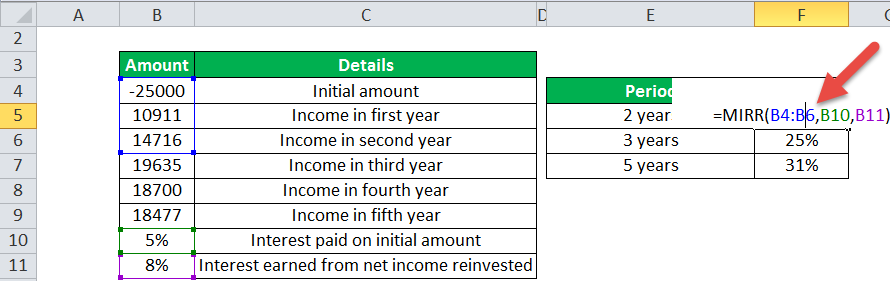
Similarly, calculate MIRR (Modified internal rate of return) after 3 and 5 years:

MIRR, after three years, will be =MIRR(B4: B7, B10, B11), and output is 25%.

MIRR, after five years, will be=MIRR(B4: B9, B10, B11), and output is 31%.

Example #2

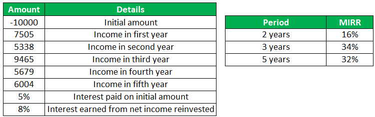
Consider an initial loan amount of 10,000 as an initial investment with an interest rate of 5% yearly, and you have earned an interest rate of 8% from the reinvested income.

Below is the table showing the income details after a regular interval. For example, the cash flow for the 1st, 2nd, 3rd, 4th, and 5th years are as follows: 7,505, 5,338, 9,465, 5,679, and 6,004.

Now calculate MIRR after 2 years:

=MIRR(B15:B17,B21,B22)and output MIRR is 16%.

Similarly, calculate MIRR after 3 and 5 years:

MIRR after three years will be =MIRR(B15: B18, B21, B22), and output is 34%.

MIRR after five years will be =MIRR(B15:B20,B21,B22) and output is 32%.

Things to Remember

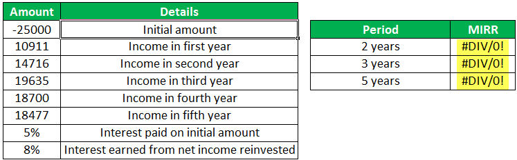
The loan amount is always considered a negative value.
After regular intervals, the modified internal return rate is always calculated on a variable cash flow.
Error handling:

#DIV/0!: MIRR excel will return #DIV/0#DIV/0! is the division error in Excel which occurs every time a number is divided by zero. Simply put, we get this error when we divide any number by an empty or zero-value cell.read more! The exception occurs when the supplied error does not contain at least one negative or positive value.

#VALUE!: MIRR will return this kind of exception when any supplied value is non-numeric.

What is MIRR?

MIRR, or “modified internal rate of return” is an Excel function that accounts for the cost of capital and reinvestment rate of the cash flows from a project or company.

How to Use the MIRR Function in Excel (Step-by-Step)

MIRR stands for the “modified internal rate of return” and attempts to measure the potential profitability (and returns) from undertaking a project or investment.

As implied by the name, the MIRR Excel function is different from the traditional IRR function in that:

Positive Cash Flows are Reinvested at the Reinvestment Rate
Negative Cash Flows (i.e. the Initial Outlay) are Discounted at the Financing Rate

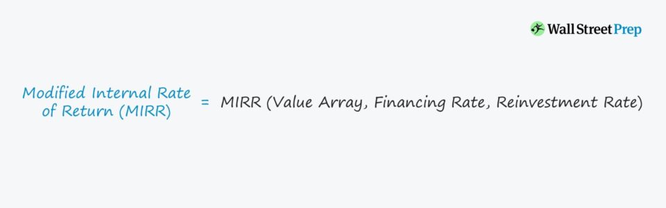
MIRR Formula

The modified internal rate of return (MIRR) formula in Excel is as follows.

MIRR Function = MIRR(values, finance_rate, reinvest_rate)

The inputs in the MIRR formula are as follows:

values: The array or range of cells with the value of the cash flows, including the initial outflow.
finance_rate: The cost of borrowing (i.e. interest rate) to fund the project or investment.
reinvest_rate: The compounding rate of return at which positive cash flows are assumed to be reinvested.

The initial outlay must be entered as a negative number in Excel for the formula to work properly.

How to Interpret MIRR vs. Cost of Capital

For purposes of capital budgeting, the following rules are generally followed:

If MIRR > Cost of Capital ➝ Accept Project
If MIRR < Cost of Capital ➝ Reject Project

When comparing numerous projects, the one with the highest MIRR is likely the one to pick, especially if other metrics also lead to the same conclusion.

Excel MIRR vs. IRR Function: What is the Difference?

The issue with the IRR Excel function is the implicit assumption that future positive cash flows are reinvested at the project or company’s cost of capital (i.e. required rate of return).

Critics of the IRR function argue that the assumption that the reinvestment rate is equal to the cost of capital overstates the return on the project or investment.

The reinvestment rate and cost of capital are often different in reality, so MIRR provides the option to specify a different reinvestment rate for future cash flows.

In effect, the MIRR Excel function is considered a more conservative measure compared to the IRR function (and usually results in a lower return).

MIRR Excel Function: Reinvestment and Financing Assumptions

One limitation to the MIRR Excel function is that it assumes 100% of cash flows are reinvested into the project/company, which is not always the case.

Hypothetically, one could adjust the reinvestment rate and financing rate for each progressive stage, but doing so brings up the issue of uncertainty around the timing of specific actions.

In other words, attempting to precisely model out the reinvestment rate, financing rate, and cost of capital for each period does not necessarily add more accuracy to the analysis due to future uncertainty.

The IRR Excel function remains frequently used due to its simplicity, however.

MIRR Calculator – Excel Model Template

We’ll now move to a modeling exercise, which you can access by filling out the form below.

MIRR Calculation Example

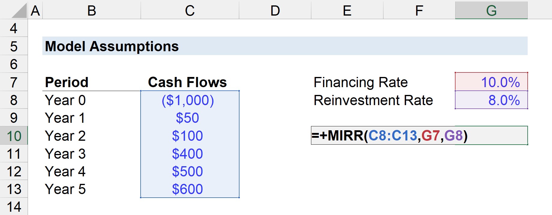
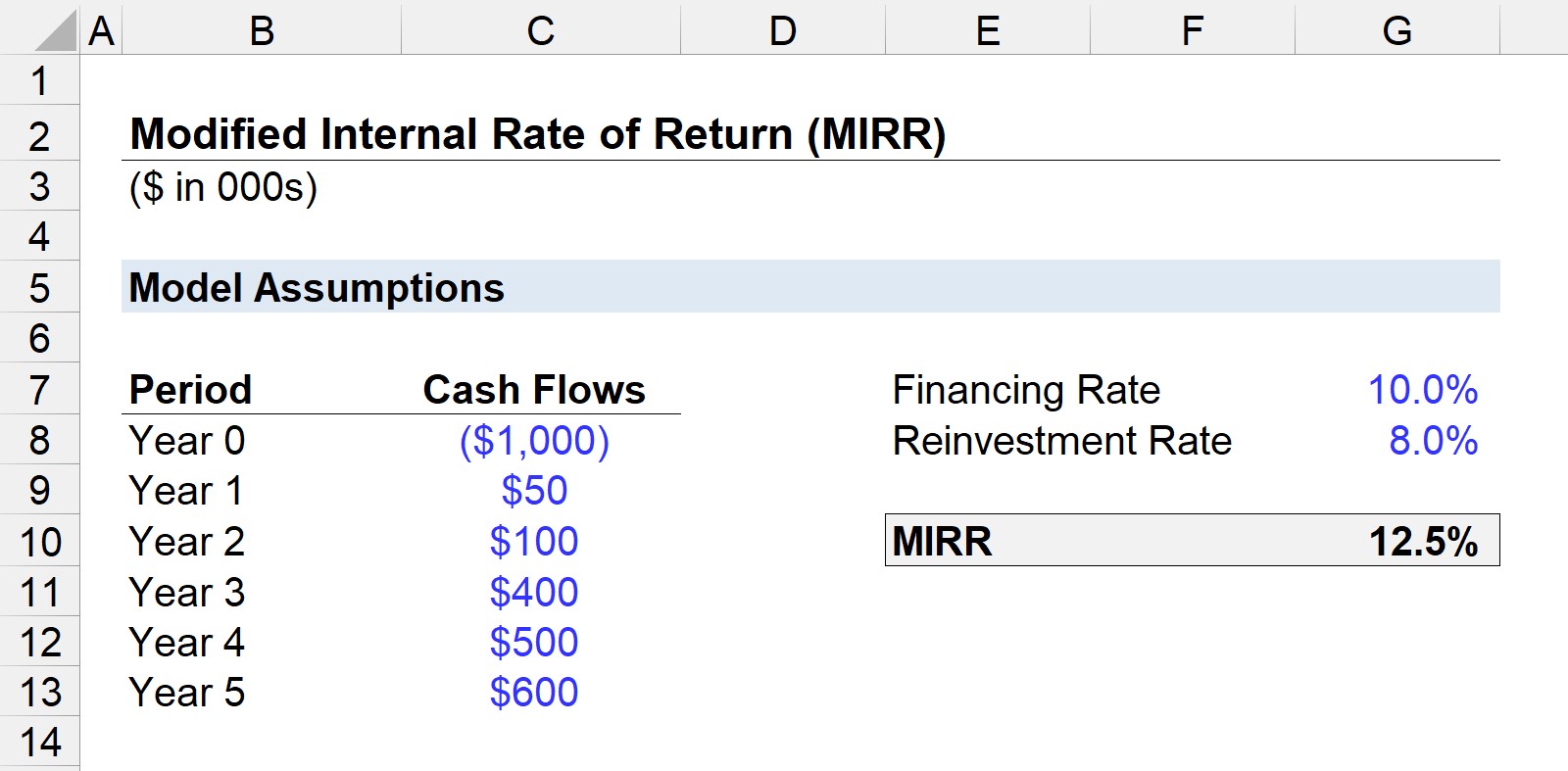
In our example scenario, we will be assuming a project has an initial cost of $1 million.

After the initial cash outlay during the initial period (Year 0), the project is projected to produce the following cash flow amounts each year:

Year 0: –$1m
Year 1: $50k
Year 2: $100k
Year 3: $400k
Year 4: $500k
Year 5: $600k

As for the financing rate and reinvestment rate, we’ll assume the following:

Financing Rate: 10%
Reinvestment Rate: 12.5%

The greater the difference between the financing rate and reinvesting rate, the more that the IRR and MIRR will diverge from each other.

If we enter the provided assumptions into the Excel formula, we get 12.5% as the MIRR.

The MIRR formula entered for our model is shown below:

Conversely, if we had used the IRR function, the resulting IRR is 14%, which demonstrates how MIRR is viewed as a more conservative measure.

But again, whether MIRR is more “accurate” or not is dependent on the amount of information on hand and the rationale behind the associated assumptions.

Turbo-charge your time in Excel
Used at top investment banks, Wall Street Prep’s Excel Crash Course will turn you into an advanced Power User and set you apart from your peers.

Learn More

Источник