
Excel for Microsoft 365 Excel for Microsoft 365 for Mac Excel for the web Excel 2021 Excel 2021 for Mac Excel 2019 Excel 2019 for Mac Excel 2016 Excel 2016 for Mac Excel 2013 Excel 2010 Excel 2007 Excel for Mac 2011 Excel Starter 2010 More…Less
This article describes the formula syntax and usage of the MID and MIDB function in Microsoft Excel.
Description
MID returns a specific number of characters from a text string, starting at the position you specify, based on the number of characters you specify.
MIDB returns a specific number of characters from a text string, starting at the position you specify, based on the number of bytes you specify.
Important:
-
These functions may not be available in all languages.
-
MID is intended for use with languages that use the single-byte character set (SBCS), whereas MIDB is intended for use with languages that use the double-byte character set (DBCS). The default language setting on your computer affects the return value in the following way:
-
MID always counts each character, whether single-byte or double-byte, as 1, no matter what the default language setting is.
-
MIDB counts each double-byte character as 2 when you have enabled the editing of a language that supports DBCS and then set it as the default language. Otherwise, MIDB counts each character as 1.
The languages that support DBCS include Japanese, Chinese (Simplified), Chinese (Traditional), and Korean.
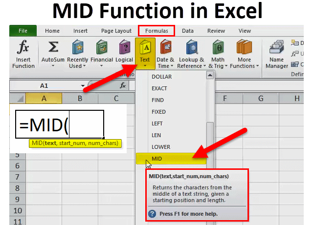
Syntax
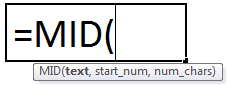
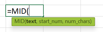
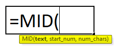
MID(text, start_num, num_chars)
MIDB(text, start_num, num_bytes)
The MID and MIDB function syntax has the following arguments:
-
Text Required. The text string containing the characters you want to extract.
-
Start_num Required. The position of the first character you want to extract in text. The first character in text has start_num 1, and so on.
-
If start_num is greater than the length of text, MID/MIDB returns «» (empty text).
-
If start_num is less than the length of text, but start_num plus num_chars exceeds the length of text, MID/MIDB returns the characters up to the end of text.
-
If start_num is less than 1, MID/MIDB returns the #VALUE! error value.
-
-
Num_chars Required for MID. Specifies the number of characters you want MID to return from text.
-
If num_chars is negative, MID returns the #VALUE! error value.
-
-
Num_bytes Required for MIDB. Specifies the number of characters you want MIDB to return from text, in bytes.
-
If num_bytes is negative, MIDB returns the #VALUE! error value.
-
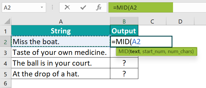
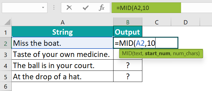
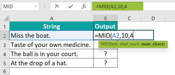
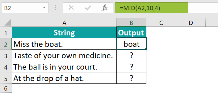
Example
Copy the example data in the following table, and paste it in cell A1 of a new Excel worksheet. For formulas to show results, select them, press F2, and then press Enter. If you need to, you can adjust the column widths to see all the data.
|
Data |
||
|
Fluid Flow |
||
|
Formula |
Description |
Result |
|
=MID(A2,1,5) |
Returns 5 characters from the string in A2, starting at the 1st character. |
Fluid |
|
=MID(A2,7,20) |
Returns 20 characters from the string in A2, starting at the 7th character. Because the number of characters to return (20) is greater than the length of the string (10), all characters, beginning with the 7th, are returned. No empty characters (spaces) are added to the end. |
Flow |
|
=MID(A2,20,5) |
Because the starting point is greater than the length (10) of the string, empty text is returned. |
Need more help?
Содержание
- Функция Mid
- Синтаксис
- Примечания
- Пример
- См. также
- Поддержка и обратная связь
- MID, MIDB functions
- Description
- Syntax
- Example
- Excel MID Function – How To Use
- Syntax
- Important Characteristics of the MID Function
- Examples of MID Function
- Example 1: Basic Functionality of the MID Function
- Example 2: Extract Substring After a Specific Character
- Example 3: Extract First or Last Name
- Extract First Name using MID Function
- Extract Last Name using MID Function
- Substring Between Two Delimiters
- Example 1 – Extracting Substring Between Two Different Delimiters
- Example 2: Extracting Substring Between Same Delimiters
- Forcing MID Function to Return Numbers
- RIGHT Function vs LEFT Function vs MID Function
- Subscribe and be a part of our 15,000+ member family!
Функция Mid
Возвращает значение типа Variant (String), содержащее указанное число символов строки.
Синтаксис
Синтаксис функции Mid состоит из следующих именованных аргументов:
| Часть | Описание |
|---|---|
| строка | Обязательный аргумент. Строковое выражение, из которого возвращаются символы. Если строка содержит значение NULL, возвращается NULL. |
| начало | Обязательный аргумент. Long. Позиция символа в строке, с которой начинается забираемая часть. Если значение аргумента начало больше, чем число символов в строке, функция Mid возвращает строку нулевой длины («»). |
| длина | Необязательный аргумент. Variant (Long). Число возвращаемых символов. Если не указано или если меньше, чем символов длины в тексте (включая символ в начале), возвращаются все символы от начальной позиции до конца строки. |
Примечания
Чтобы определить число символов в строке, используйте функцию Len.
Используйте функцию MidB для работы с содержащимися в строке байтами, например в языках с двухбайтовыми кодировками (DBCS). Вместо указания числа символов аргументы задают число байтов. Образец кода с использованием функции MidB приведен во втором примере.
Пример
В первом примере с помощью функции Mid возвращается указанное количество знаков строки.
Во втором примере с использованием функции MidB и определяемой пользователем функции (MidMbcs) также возвращаются знаки из строки. Отличие от первого примера состоит в том, что исходная строка представляет собой строку ANSI и ее длина выражена в байтах.
См. также
Поддержка и обратная связь
Есть вопросы или отзывы, касающиеся Office VBA или этой статьи? Руководство по другим способам получения поддержки и отправки отзывов см. в статье Поддержка Office VBA и обратная связь.
Источник
MID, MIDB functions
This article describes the formula syntax and usage of the MID and MIDB function in Microsoft Excel.
Description
MID returns a specific number of characters from a text string, starting at the position you specify, based on the number of characters you specify.
MIDB returns a specific number of characters from a text string, starting at the position you specify, based on the number of bytes you specify.
These functions may not be available in all languages.
MID is intended for use with languages that use the single-byte character set (SBCS), whereas MIDB is intended for use with languages that use the double-byte character set (DBCS). The default language setting on your computer affects the return value in the following way:
MID always counts each character, whether single-byte or double-byte, as 1, no matter what the default language setting is.
MIDB counts each double-byte character as 2 when you have enabled the editing of a language that supports DBCS and then set it as the default language. Otherwise, MIDB counts each character as 1.
The languages that support DBCS include Japanese, Chinese (Simplified), Chinese (Traditional), and Korean.
Syntax
MID(text, start_num, num_chars)
MIDB(text, start_num, num_bytes)
The MID and MIDB function syntax has the following arguments:
Text Required. The text string containing the characters you want to extract.
Start_num Required. The position of the first character you want to extract in text. The first character in text has start_num 1, and so on.
If start_num is greater than the length of text, MID/MIDB returns «» (empty text).
If start_num is less than the length of text, but start_num plus num_chars exceeds the length of text, MID/MIDB returns the characters up to the end of text.
If start_num is less than 1, MID/MIDB returns the #VALUE! error value.
Num_chars Required for MID. Specifies the number of characters you want MID to return from text.
If num_chars is negative, MID returns the #VALUE! error value.
Num_bytes Required for MIDB. Specifies the number of characters you want MIDB to return from text, in bytes.
If num_bytes is negative, MIDB returns the #VALUE! error value.
Example
Copy the example data in the following table, and paste it in cell A1 of a new Excel worksheet. For formulas to show results, select them, press F2, and then press Enter. If you need to, you can adjust the column widths to see all the data.
Returns 5 characters from the string in A2, starting at the 1st character.
Returns 20 characters from the string in A2, starting at the 7th character. Because the number of characters to return (20) is greater than the length of the string (10), all characters, beginning with the 7th, are returned. No empty characters (spaces) are added to the end.
Because the starting point is greater than the length (10) of the string, empty text is returned.
Источник
Excel MID Function – How To Use
The MID function returns a specific number of characters from the middle of the string after we state the starting position and the number of characters to extract. The MID Function in Excel is one of the text functions that allows us to get a substring from a stringtext as per our requirement
It is one of the most useful functions when we want to extract the middle name from the full name, the domain name from email IDs, or any substring between two characters.

Table of Contents
Syntax
The syntax of the MID function is as follows:
The MID function in Excel accepts three arguments and all three arguments are mandatory.
Arguments:
‘text‘ – This holds the value of the input text/string. A cell reference containing the input string or text enclosed in double quotes are both acceptable input values.
‘start_num‘ – The position of the first character we want to extract. It must be an integer/formula which indicates the starting position of the extraction.
‘num_chars‘ – Number of characters we wish to extract from the starting point. The num_chars argument indicates the character length of the return value.
Important Characteristics of the MID Function
One of the essential and basic characteristics of the MID function being a text function is that it always returns a text value regardless of the input value. Even if the retrieved substring is only made up of numbers, it will be in text format. Other important MID function features are as follows:
- If the value of start_num exceeds the length of input text, the MID function returns «» (empty text).
- If the start_num value is less than 1, the function returns a #VALUE! error.
- If the value of num_chars is a negative number, the MID function gives a #VALUE error.
- If the num_chars value is less than 1, then the MID function’s return value is an empty string, a blank cell.
Last of all, if the sum of the value of start_num and num_chars is greater than the total input text length, the MID function returns all the characters from start_num to the last character. This characteristic comes in very handy for certain conditions. We will find out in the examples below.
Examples of MID Function
The MID function can be used independently or can be combined with various other Excel functions such as SEARCH, FIND, LEN, and more. Let’s go through some examples to fully comprehend the usage and utility of the MID function.
Example 1: Basic Functionality of the MID Function
In the below example, we have taken 3 different instances and tried using the basic MID function.

In the first case, the input text/string is a full name ‘Cassie Martha Soros’ where we wish to extract the middle name –»Martha». So, using the MID function we apply the formula:
Here, the first parameter text is the cell reference B3. The second parameter start_num is the starting position which is 8 as the first name is 6 characters long, the space is the 7 th character and then we add 1 so that we reach the beginning of the middle name. Lastly, the third argument num_chars is the number of characters of the middle name which is 6.
The second instance is where we are trying to extract the house number and street address from the complete address in cell B4. We are checking if the MID function counts a special character (,) and also whether the MID function can return characters from the beginning of the text or only from the middle. The formula goes as follows:
The first parameter is B4, the input text. The second parameter is 1 as the house number is in the beginning. Finally, the third parameter is 13 which is the house number (3 characters long) combined with a comma, a space character, and then the street name which is 8 characters long. Hence our output, in this case, becomes ‘220, Kisvagen’.
In the last example, the input text is in cell B5, which is actually a number 123456789. To extract 4 digits from the second position, the formula would be:
Here, the output value is left aligned. Is it a text value? We have something to learn here, which we will find in the section below.
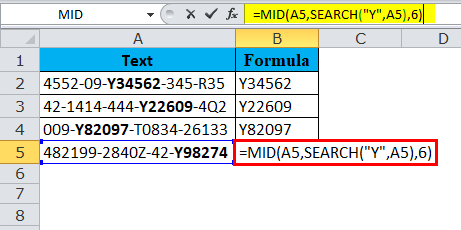
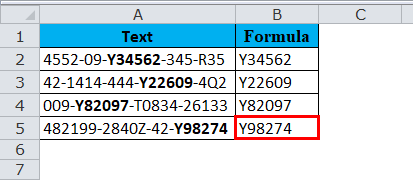
In the following example, we are trying to extract a substring from the input text after a special character. The dataset in column B in this example consists of Employee IDs; a combination of the department name, and a unique ID followed by the employee’s date of birth.
For instance, in the Employee ID TECH-1234-08051990, the employee belongs to the tech team, the unique ID is 1234, and the date of birth is 08 May 1990.
We want to extract the unique ID from each Employee ID. Using the MID function, we can extract it from the input string, but the issue is that the character length of the department name varies. Resultantly, the value of start_num varies.

Lucky for us, the department name is followed by a hyphen ‘-‘, and the employee ID is 4 characters long. Now, we can use the MID function combined with the FIND function. The FIND function will locate the hyphen’s ‘-‘ position, which will be the input value of start_num.
Use the FIND function as follows:
This formula locates the hyphen in B3 and returns 4 (the hyphen is the 4th character in B3). To use the FIND function as an input value for the start_num parameter, we must add 1 to this result because the unique ID begins from the 5th character of the text string and we don’t want to see the hyphen in the final result.
The value of num_chars shall be 4 as all the unique IDs in our example are 4-digit numbers. So, combining the FIND and MID functions, the final function is as follows:
And here’s how this formula extracts the unique IDs for us:

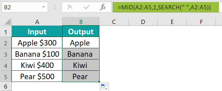
Imagine we have a data set of peoples’ names and are asked to extract first, middle and last names in different columns. Usually, we would want to use the LEFT function for the first name and the RIGHT function for the last name. However, the functionality of two different functions can be accomplished using the MID function alone.
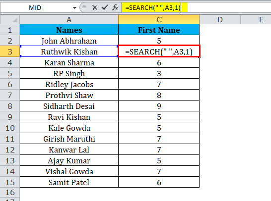
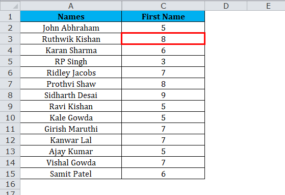
Let’s learn how to extract first and last names using the MID function. We cannot simply use the MID function as the starting position for separating last names as the number of characters will vary for each name. Ergo, we will use the SEARCH function to our advantage and then merge it with the MID function.
We could have used the earlier mentioned FIND function too, but as we have understood the functionality of the FIND function, let’s try to learn the MID function with the SEARCH function here. Also, the SEARCH function is case insensitive and that will make our task even easier.
The first and last names are divided by a space, a common pattern we can make use of. The beginning position in the MID function will be the starting of the string, whereas the number of characters can be determined using the SEARCH function.
The position of the space » » is where the first name ends and hence, is the number of characters to be extracted. The space character is located in the name using the SEARCH function, which returns its position, from which we deduct 1 to delete the inclusion of the extra space.
Let’s try to put this logic in the form of an Excel formula.
Seeing the example ahead, the first name in cell B3 is ‘Simon Rogers’. If we used the MID function only on this cell, we would try:
However, this formula will not give us the required result for all other cells since all the names won’t be 5 letters.
Let’s generalize it so we can use it for the complete dataset.

As the first parameter, start_num remains the same for all the names,. To determine the second parameter, we must find the position of the space. To find the position of the space » » using the SEARCH function, the formula will go as follows:
Combining it with the MID function, the formula will become:
To remove the extra trailing space, subtract 1 from the position. The final formula will be:

Furthermore, can we use the same logic to extract the last name? Let’s find out.
To pull out the last name using the MID function, we can use the SEARCH function to point out the start_num parameter as the last name begins after the space. How to find the number of characters (num_chars) to extract?
As mentioned earlier, if the total of the start_num and num_chars is more than the length of the string, the MID function returns the remaining string from the start_num. So, utilizing that to our advantage, there are two ways to use the MID function.
The first one is fairly simple. Assuming that the total character length of names will never exceed 1000, we can assign 1000 to the num_chars parameter.
The SEARCH function will determine the position of the space » » using the formula:
This will be the input value of the first parameter start_num. Assigning 1000 to the second parameter, the formula will become:

To remove the extra leading spaces from the extracted last names, use the TRIM function. The final MID function will be used as follows:
Now we have the last names extracted by the MID and SEARCH functions and leading spaces removed by the TRIM function:

The second way is more elegant. Instead of an assumed number in the num_chars parameter, we can use the LEN function to determine the total length of the name and use that value in the num_chars parameter.
Combining the LEN & SEARCH functions with the MID function, the formula will be as follows:
Here, LEN function will return the total length of the input string, and SEARCH function will extract the position of the space » » in the string. The ultimate effect is similar to what we have seen in the previous formula. The location of the space character added to the total characters of B3 will obviously be more than the total characters in B3.

To polish it further, we can use the TRIM function to eliminate all the extra spaces.

Substring Between Two Delimiters
After practicing the above examples, we can extract a substring from a string after determining the position of the space » » or any other special character. Now, what if the input string is long with several delimiters? Just for clarity, one or more characters that divide text strings are known as delimiters, such as space ( ), quotes («), commas (,), semicolons (;), slashes (/) or pipes (|).
When we dive in further, there are two scenarios of extracting a substring from an input string between delimiters; first when they are different and second when the delimiters are the same. Let’s understand both cases using an example.
Let’s assume we have a set of email IDs, and for research purposes, we want to extract the domain name from each email ID to analyze which one is most preferred. The email ID structure goes as follows ‘[email protected]’, where ‘learning’ is a username and gmail is a domain name.

As we can see, we have two different delimiters (@) and (.) separating the domain name (gmail) from the rest of the string (username). So, to pull out the substring, we must locate the position of two delimiters where the first delimiter is the starting position (start_num), and using the second delimiter, we can calculate the number of characters to be extracted.
As we already know, the MID function consists of three arguments. The first argument is the cell reference to email ID (B3). The second argument is the starting position which can be calculated using the SEARCH function:
This formula will give us the position of the first delimiter (@). As we require the starting position to be one character after (@), we add 1.
Lastly, for the third argument (num_chars), we need the number of characters to be extracted. We can find the location of the second delimiter (.) and then subtract the position of the first delimiter. The formula goes as follows:
To finalize and remove the trailing space, subtract 1.
Putting it all together, the final MID function formula to extract the substring from two different characters is:
This is how our experiment turned out:

In the above examples, we already know how to extract the first and last name from the full name using the MID function. However, what about the middle name? We cannot simply use the basic MID function as the character length of middle names varies for each person.
However, in the previous example, we learned how to extract a substring between two delimiters.
As we will notice, there is a space ( ) before and after the middle name, separating it from the first & last name. We can find the position of two delimiters (in this case, both the delimiters are space characters) and extract the middle name from the full name.
In the given dataset in column B, we have the list of full names. Let’s take the example of the first name in cell B3.

The first parameter of the MID function is the input text which is cell B3. For the second parameter, that is start_num, if we find the position of the space before the middle name and then add 1 to it, we should have our argument input. Using the SEARCH function, the position of the first space » » can be determined using the following formula:
This returns 7 and if we do a quick count check, indeed the middle name’s first letter is the 7 th character of the text string.
Easy enough, right?
Now, to determine the number of characters to be returned, we can find the position of the second space » » (after the middle name) and subtract the position of the first space from it.
Remember, the SEARCH function has an additional third optional parameter start_num stating the starting position of the search within the string. This will come in handy here as there are two spaces in this text (full name). To find the position of the second space, the formula goes as follows:
Explaining further, we are telling the SEARCH function to find » » in B3 starting after the position of the first space. If we don’t use the nested SEARCH function, it will keep returning the position of the first space, and we don’t want that, do we?
This formula returns 11 which you can tally again. Now that we have the position of both the space characters 11-7 is the number of characters to extract. Combining all to finish our MID function, the formula goes as follows:
The MID function will return 4 characters from B3 starting from the character after the first space. The result is Dona and the rest can be seen below:

Forcing MID Function to Return Numbers
Like other text functions in Excel, the output value of the MID function is always in text format. Even if the input or output value contains only digits and looks like a number format, it is indeed in text format.
There are two ways to find if the output value is in text or number format. One is the innate nature of Excel to left align a text and right align a number. The second is to use the ISNUMBER function.
In this example, we multiply 99 with 200 and then extract the 2 digit of the result, starting from the second position. Using the MID function, the formula goes as follows

We know that 99*200 is 19800. We are trying to extract 2 digits out of it starting from the 2nd position and hence the result is 98.
However, if you notice the result here is left aligned. By default Excel aligns all the numbers to right and text to left. This hints that the result here is a text instead of a number.
This can be further proved with the ISNUMBER function, which also returns false implying that the result of the MID function is not a number.
To ensure that the MID function returns a number, use the VALUE function, which transforms a text value representing a number into a number. Wrap the MID function inside the VALUE function. The formula used will be:

As evident from the example, the return value of the MID function combined with the VALUE function is right aligned, and when checked with ISNUMBER function, the result is TRUE.
RIGHT Function vs LEFT Function vs MID Function
We have now understood several ways to use the MID function for various tasks. Similar to the MID function, there are two more text functions in Excel; LEFT & RIGHT functions. For better comprehension, we will attempt to use all three Excel functions on the same input string in the following example.
In this example, we have taken an input text/string in cell A2 «Smart, Easy & Effective»

We have used the LEFT function to extract the first word of the string «Smart». As it is 5 characters long, the LEFT function formula will be:
Unlike the MID function, the LEFT function doesn’t have the start_num argument since the starting point is automatically the first character from the left. The same is the case with the RIGHT function. It just extracts characters from right to left.
Similarly, we’ve used the RIGHT function on the input string to extract the last word «Effective» (9 characters long). The formula is:
Now the function that we know very well; the MID function. The formula used to extract the middle word «Easy» will be:
With that, we’ve discussed the ins and outs of the MID function. There are numerous other interesting things the MID function can manage such as returning a word beginning with a certain character (e.g. social media tags with the @ symbol such as @cholecakes, @popartillustrations), returning the nth word from a text string, and so on. Keep practicing and explore new ways to use the MID function.
Subscribe and be a part of our 15,000+ member family!
Now subscribe to Excel Trick and get a free copy of our ebook «200+ Excel Shortcuts» (printable format) to catapult your productivity.
Источник
The MID function in Excel is a text function used to find out strings and return them from any middle part of the Excel. This formula extracts the result from the text or the string itself, the start number or position, and the string’s end position.
For example, suppose we have a table of products from A2:A5: “Dolls,” “Barbie,” “Bottle,” and “Pen.” in the worksheet. We need to fetch the substring from the given substring. When we type, =MID(A2,2,4) returns “oll.” It will bring the substring from 2 characters and 4 letters from the 2nd position.
In simple words, the MID function in Excel extracts a small part of the string from the input string or returns a required number of characters from text or string.
Table of contents
- MID in Excel
- MID Formula in Excel
- How to Use MID Function in Excel? (with Examples)
- MID in Excel as a worksheet function.
- Example #1
- Example #2
- Example #3
- Example #4
- Excel MID Function can be used as a VBA function.
- Things to Remember About Excel MID Function
- MID Excel Function Video
- Recommended Articles
MID Formula in Excel
The MID formula in excel has three compulsory parameters, i.e., text, start_num, num_chars.
Compulsory Parameters:
- text: It is a text from which you want to extract the substring.
- start_num: The starting position of the substring.
- num_chars: The numbers of characters of the substring.
How to Use MID Function in Excel? (with Examples)
The MID function in Excel is very simple and easy to use. Let us understand the working of the MID function in Excel by some MID formula examples. The MID function can be used as a worksheet function and VBA function.
You can download this MID Function Excel Template here – MID Function Excel Template
MID in Excel as a worksheet function.
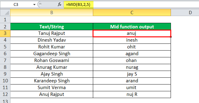
Example #1
In this MID formula example, we are fetching the substring from the given text string using the MID formula in excel =MID(B3,2,5). It will bring the substring from 2 characters and 5 letters from the 2nd position, and the output will be as shown in the second column.
Example #2
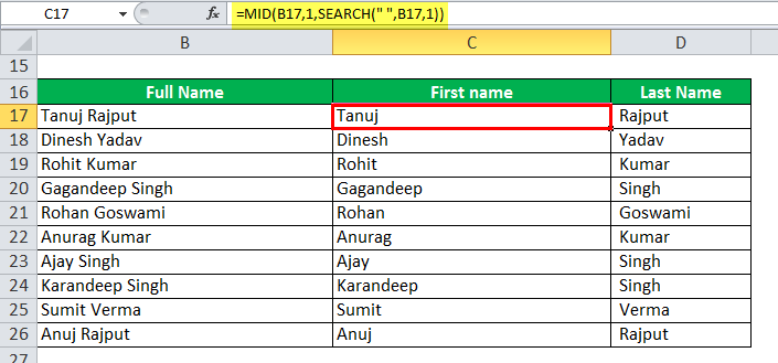
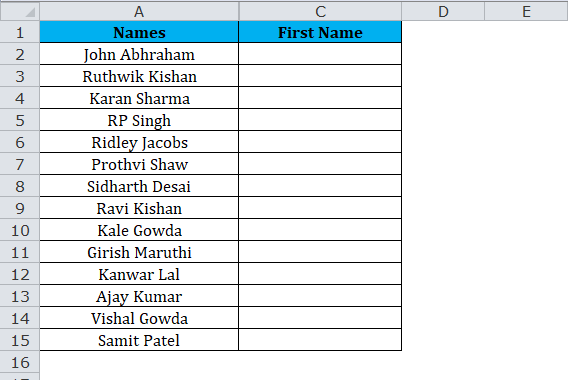
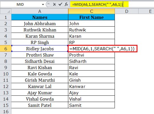
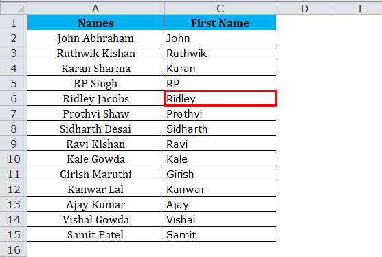
We can use the mid function that extracts the first and last names from the full names.
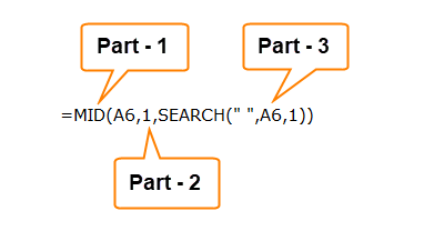
For First Name: here we have used the MID formula in Excel =MID(B17,1,SEARCH(” “,B17,1)); in this MID Formula example, the MID function searches the string at B17 and starts the substring from the first character, here search function fetches the location of space and return the integer value. In the end, both functions filter out the first name.
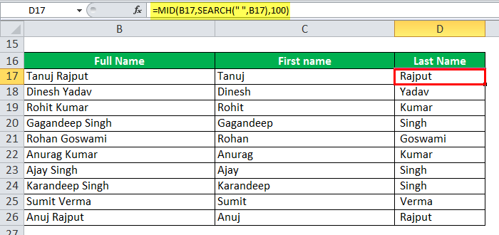
For the Last Name: Similarly, for the last name, use the =MID(B17,SEARCH(” “,B17),100), and it will give you the last name from the full name.
Example #3
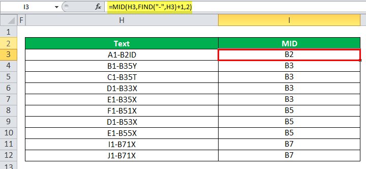
Suppose we have to find out the block from ID, which is located after “-“in ID, then use =MID(H3,FIND(“-“,H3)+1,2) MID formula in Excel to filter out the block ID two-character after.
Example #4
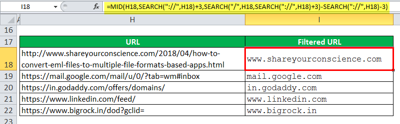
We can also find out the domain name from the web URLs. Here is the MID function used to achieve this:
=MID(H18,SEARCH(“://”,H18)+3,SEARCH(“/”,H18,SEARCH(“://”,H18)+3)-SEARCH(“://”,H18)-3)
Excel MID Function can be used as a VBA function.
Dim Midstring As String
Midstring = Application.worksheetfunction.mid(“Alphabet”, 5, 2)
Msgbox(Midstring) // Return the substring “ab” from string “Alphabet” in the message box.
The output will be “ab.”
Things to Remember About Excel MID Function
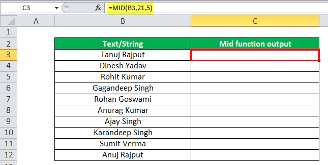
- Excel MID formula returns empty text if the start_num is greater than the length of the string.
=MID(B3,21,5)= blank as the start number is greater than the string length, so the output will be empty, as shown below.
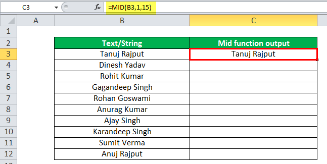
- If start_num is < the length of text, but start_num + num_chars exceeds the length of the string, then MID returns the characters up to the end of the text.
=MID(B3,1,15)
- The MID function in Excel through the #VALUE#VALUE! Error in Excel represents that the reference cell the user has either entered an incorrect formula or used a wrong data type (mostly numerical data). Sometimes, it is difficult to identify the kind of mistake behind this error.read more! Error
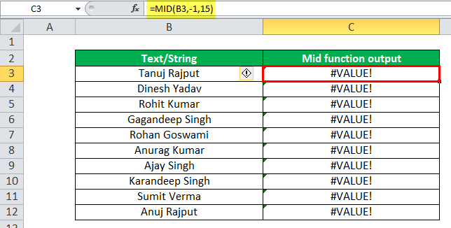
- If start_num < 1 ex. =MID(B3,-1,15)
- If num_chars is a negative value.
=MID(B3,1,-15)

MID Excel Function Video
Recommended Articles
This article is a guide to MID Function in Excel. We discuss the MID formula in Excel and how to use the MID Excel formula along with the MID formula example and downloadable Excel templates. You may also look at these useful functions in Excel: –
- VBA MIDVBA MID function extracts the middle values from the supplied sentence or word. It is categorized under the String and Text function and is a worksheet function.read more
- INDEX FunctionThe INDEX function in Excel helps extract the value of a cell, which is within a specified array (range) and, at the intersection of the stated row and column numbers.read more
- RAND Excel FunctionThe RAND function in Excel, also known as the random function, generates a random value greater than 0 but less than 1, with an even distribution among those numbers when used on multiple cells. read more
- POWER in ExcelPOWER function calculates the power of a given number or base. To use this function you can use the keyword =POWER( in a cell and provide two arguments one as number and another as power.read more
- Frequency Distribution in ExcelFrequency distribution in excel is a calculation of the rate of a change happening over time in the data. By categorizing data in sets and applying the array formula frequency function or in the data analysis tab, use the histogram tool to determine frequency distribution.read more
На чтение 1 мин
Функция ПСТР (MID) в Excel используется для отображения куска текста из строки по заданному количеству символов.
Содержание
- Что возвращает функция
- Синтаксис
- Аргументы функции
- Дополнительная информация
- Примеры использования функции ПСТР в Excel
Что возвращает функция
Возвращает часть строки из текста.
 Больше лайфхаков в нашем Telegram Подписаться
Синтаксис
=MID(text, start_num, num_chars) — английская версия
=ПСТР(текст;начальная_позиция;число_знаков) — русская версия
Аргументы функции
- text (текст) — текст из которого вы хотите отобразить часть;
- start_num (начальная_позиция) — стартовая позиция внутри текста, с которой будет производиться отображение части текста;
- num_chars (число_знаков) — суммарное количество символов, которое вы хотите отобразить из заданного текста.
Дополнительная информация
- Функция учитывает пробелы как отдельные символы;
- Для того, чтобы удалить лишние пробелы из текста, используйте функцию СЖПРОБЕЛЫ;
- Если стартовая позиция, с которой должно начаться отображение части текста больше чем количество символов в тексте, то функция вернет пустую ячейку;
- Функция выдаст ошибку, если стартовая позиция меньше «1» или равно отрицательному значению.
Примеры использования функции ПСТР в Excel
Purpose
Extract text from inside a string
Return value
The characters extracted.
Usage notes
The MID function extracts a given number of characters from the middle of a supplied text string. MID takes three arguments, all of which are required. The first argument, text, is the text string to start with. The second argument, start_num, is the position of the first character to extract. The third argument, num_chars, is the number of characters to extract. If num_chars is greater than the number of characters available, MID returns all remaining characters.
Examples
The formula below returns 3 characters starting at the 5th character:
=MID("The cat in the hat",5,3) // returns "cat"
This formula will extract 3 characters starting at character 16:
=MID("The cat in the hat",16,3) // returns "hat"
If num_chars is greater than remaining characters, MID will all remaining characters:
=MID("apple",3,100) // returns "ple"
MID can extract text from numbers, but the result is text:
=MID(12348,3,4) // returns "348" as text
Related functions
Use the MID function to extract from the middle of text. Use the LEFT function to extract text from the left side of a text string and the RIGHT function to extract text starting from the right side of text. The LEN function returns the length of text as a count of characters. Use FIND or SEARCH to locate an unknown start position.
Notes
- num_chars is optional and defaults to 1.
- MID will extract text from numeric values, but the result is text
- Number formatting is not counted or extracted.
The Excel MID function extracts a given number of characters from the middle of a supplied text string. For example, =MID(“apple”,2,3) returns “ppl”. The Excel LEN function returns the length of a given text string as the number of characters.
Contents
- 1 How do you use Find and mid in Excel?
- 2 Why MID is used in Excel?
- 3 How do you middle word in Excel?
- 4 What is mid formula?
- 5 How do you use mode in Excel?
- 6 How do you put text in the middle of a cell in Excel?
- 7 What is right formula in Excel?
- 8 How do I copy only part of a cell in Excel?
- 9 What is the difference between mode sngl and mode mult?
- 10 How do you use mode?
- 11 What is mode formula?
- 12 How do I select only certain characters in Excel?
- 13 How do I extract date from datetime in Excel?
- 14 What is concatenate in Excel?
- 15 How does a VLOOKUP work?
- 16 What does Num_chars mean in Excel?
- 17 How do you copy a partial text in Excel?
- 18 How do you use concatenate?
- 19 What is mode multi?
- 20 How do you use the mode sngl function?
How do you use Find and mid in Excel?
Here’s the trick: You use the Find function to return the position of the dash in the string, and you use the Find function itself as the Mid function’s first argument. As Figure B shows, the function =Find(“-“,A2) returns the value 6, since the dash appears in the sixth position of the string in A2.
Why MID is used in Excel?
Generally speaking, the MID function in Excel is designed to pull a substring from the middle of the original text string. Technically speaking, the MID function returns the specified number of characters starting at the position you specify.
How do you middle word in Excel?
To pick the Middle name from the list. We write the “MID” function along with the “SEARCH” function. Select the Cell C2, write the formula =MID(A2,SEARCH(” “,A2,1)+1,SEARCH(” “,A2,SEARCH(” “,A2,1)+1)-SEARCH(” “,A2,1)) it will return the middle name from the cell A2.
What is mid formula?
Mid function in excel is a type of text function which is used to find out strings and return them from any mid part of the excel, the arguments this formula takes is the text or the string itself and the start number or position of the string and the end position of the string to extract the result.
How do you use mode in Excel?
Use a function to find the mode in Microsoft Excel
- Step 1: Type your data into one column.
- Step 2: Click a blank cell anywhere on the worksheet and then type “=MODE.
- Step 3: Change the range in Step 2 to reflect your actual data.
- Step 4: Press “Enter.” Excel will return the solution in the cell with the formula.
How do you put text in the middle of a cell in Excel?
Align text in a cell
- Select the cells that have the text you want aligned.
- On the Home tab choose one of the following alignment options:
- To vertically align text, pick Top Align , Middle Align , or Bottom Align .
- To horizontally align text, pick Align Text Left , Center , or Align Text Right .
What is right formula in Excel?
The Microsoft Excel RIGHT function extracts a substring from a string starting from the right-most character. The RIGHT function is a built-in function in Excel that is categorized as a String/Text Function. It can be used as a worksheet function (WS) and a VBA function (VBA) in Excel.
How do I copy only part of a cell in Excel?
Paste Special options
- Select the cells that contain the data or other attributes that you want to copy.
- On the Home tab, click Copy .
- Click the first cell in the area where you want to paste what you copied.
- On the Home tab, click the arrow next to Paste, and then select Paste Special.
- Select the options you want.
What is the difference between mode sngl and mode mult?
SNGL is different from MODE. MULT function as the MODE. SNGL function returns the lowest mode, whereas the MODE. MULT function returns an array of all the modes.
How do you use mode?
To find the mode, or modal value, it is best to put the numbers in order. Then count how many of each number. A number that appears most often is the mode.
What is mode formula?
In statistics, the mode formula is defined as the formula to calculate the mode of a given set of data. Mode refers to the value that is repeatedly occurring in a given set and mode is different for grouped and ungrouped data sets. Mode = L+h(fm−f1)(fm−f1)−(fm−f2) L + h ( f m − f 1 ) ( f m − f 1 ) − ( f m − f 2 )
How do I select only certain characters in Excel?
To extract the leftmost characters from a string, use the LEFT function in Excel. To extract a substring (of any length) before the dash, add the FIND function. Explanation: the FIND function finds the position of the dash. Subtract 1 from this result to extract the correct number of leftmost characters.
Extract date from a date and time
- Generic formula. =INT(date)
- To extract the date part of a date that contains time (i.e. a datetime), you can use the INT function.
- Excel handles dates and time using a scheme in which dates are serial numbers and times are fractional values.
- Extract time from a date and time.
What is concatenate in Excel?
The word concatenate is just another way of saying “to combine” or “to join together”. The CONCATENATE function allows you to combine text from different cells into one cell. In our example, we can use it to combine the text in column A and column B to create a combined name in a new column.
How does a VLOOKUP work?
The VLOOKUP function performs a vertical lookup by searching for a value in the first column of a table and returning the value in the same row in the index_number position. The VLOOKUP function is a built-in function in Excel that is categorized as a Lookup/Reference Function.
What does Num_chars mean in Excel?
The second argument, called num_chars, specifies the number of characters to extract. If num_chars is not provided, it defaults to 1. If num_chars is greater than the number of characters available, RIGHT returns the entire text string.
How do you copy a partial text in Excel?
Here is how to do this:
- Select the cells where you have the text.
- Go to Data –> Data Tools –> Text to Columns.
- In the Text to Column Wizard Step 1, select Delimited and press Next.
- In Step 2, check the Other option and enter @ in the box right to it.
- In Step 3, General setting works fine in this case.
- Click on Finish.
How do you use concatenate?
There are two ways to do this:
- Add double quotation marks with a space between them ” “. For example: =CONCATENATE(“Hello”, ” “, “World!”).
- Add a space after the Text argument. For example: =CONCATENATE(“Hello “, “World!”). The string “Hello ” has an extra space added.
What is mode multi?
The Microsoft Excel MODE. MULT function returns a vertical array of the most frequently occurring numbers found in a set of numbers. This function is useful if there is more than one number that occurs the most. TIP: If this formula is entered as an array formula, it will return multiple modes.
How do you use the mode sngl function?
The Excel MODE. SNGL function returns the most frequently occurring number in a numeric data set. For example, =MODE. SNGL(1,2,4,4,5,5,5,6) returns 5.
Notes
- If supplied data does not contain duplicate numbers, MODE.SNGL returns #N/A.
- MODE.
- Arguments can be numbers, names, arrays, or references.
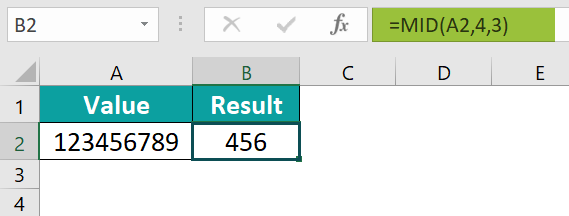
What Is MID Function In Excel?
The MID Excel function returns a specified number of characters from the middle of a given text string. Also, the MID function can be used with VALUE, SUM, COUNT, DATE, DAY, and other functions.
The MID Excel function is available under the Excel TEXT functions group.
For example, the below table shows the value in cell A2. Now, we need to apply MID function to detect the output.
The steps used to apply MID excel function are as follows:
Step 1: To begin with, select the cell to display the output. In our example, the cell is B2.
Step 2: Next, enter the complete formula =MID(A2,4,3)
Step 3: Then, press Enter key.
The function has returned the output as shown in the below image.
Likewise, we can apply MID function to obtain the middle value.
Table of contents
- What is MID Function in Excel?
- MID() Excel Formula
- How to Use MID Excel Function? (With Steps)
- #1 – Access from the Excel Ribbon
- #2 – Enter the Worksheet Manually
- Basic Example
- Examples
- Example #1 – Extracts the First and Last Names from the Full Names
- Example #2 – Find Out the Domain Name from the Web URLs
- Example #3 – Extracting Last n Digits from Some Numbers
- Example #4 – MID Function with Arrays
- Things to Remember
- Frequently Asked Questions (FAQs)
- Download Template
- Recommended Articles
- The syntax of the MID excel function is =MID(text,start_num,num_chars) where,
- text denotes the original text string.
- start_num indicates the integer that specifies the position of the first character we want to be returned.
- num_chars shows the number of characters, starting with start_num, to be returned from the start of the text. It is the number of characters to be extracted.
- If the user does not specify the last parameter of the MID function, it will take 0 by default.
- The number formatting is not the part of a string and cannot be extracted or counted.
MID() Excel Formula
The syntax of the MID excel formula is:
where,
- text: It denotes the original text string.
- start_num: It indicates the integer specifying the position of the first character we want to be returned.
- num_chars: It shows the number of characters, starting with start_num, to be returned from the start of the text. It is the number of characters to be extracted.
Unlike other functions, all the arguments are mandatory in MID excel formula.
How To Use MID Excel Function? (With Steps)
#1 – Access From The Excel Ribbon
- Choose the empty cell to display the result.
- Go to the Formulas tab.
- Select Text from the menu.
- Select MID from the drop-down menu.
- The Function Arguments window appears.
- Based on the number of arguments, enter the value in the Text, Start_num, and Num_chars.
- Select OK.
#2 – Enter The Worksheet Manually
- Select an empty cell for the output.
- Type =MID( in the selected cell. Alternatively, type =M and double-click the MID function from the list of suggestions shown by Excel.
- Enter the arguments as cell references or direct values.
- Close the parenthesis and press the Enter key.
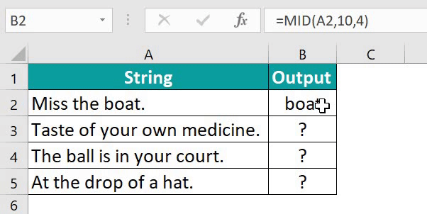
Let us take a basic example to understand this function. The following table shows the strings in column A. Now, we need to extract the text from the string using MID excel function.

The steps to extract the text from the string using MID Excel function are as follows:
- To begin with, select the column to display the result. The selected column, in this case, is column B.
- Next, enter the MID excel function formula in cell B2.
Select the cell A2 in the text argument.

Enter the value as 10 in the start_num argument.

Enter the value ‘4’ in the num_chars argument.
So, the complete formula is =MID(A2,10,4).
- Then, press Enter key.
We can see that the function has returned ‘boat’ in cell B2.
- Drag the cursor to cell B5 using AutoFill option.

Likewise, we can use MID function to extract mid values.
Examples
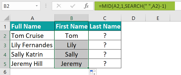
Example #1 – Extracts The First And Last Names From The Full Names
The below table shows the full name of various people in column A. We need to extract the first name and the last name from the given table array using MID Excel function.

The steps to extract the text from the string by the MID in Excel are as follows:
Step 1: To begin with, select the column to display the cell. In this example, we will enter the First name in column B and the Last name in column C.
Step 2: Next, enter the MID formula in cell B2 for extracting the first name.
Step 3: Now, enter the value for the text argument as A2.
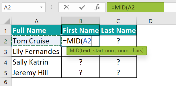
Step 4: The value entered for the start_num argument is 1.

Step 5: The value entered for num_chars argument is the SEARCH formula as we extract the first name.
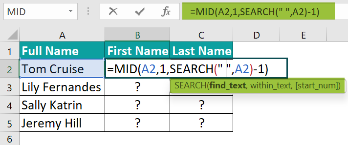
Step 6: The entered complete formula in cell B2 for extracting the first name is =MID(A2,1,SEARCH(“ ”,A2)-1)
Press Enter key.
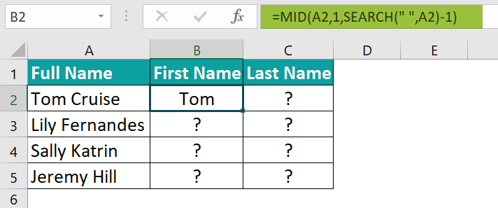
Step 7: The result is returned as Tom.
Next, drag the cursor to cell B5; all the first name from the data is extracted in column B as shown in the following image.
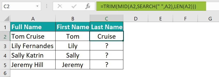
Step 8: Next, enter the MID formula in cell C2 for extracting the Last name.
Step 9: Firstly, we will enter the TRIM excel formula, and then the MID formula value entered for the text argument is A2.
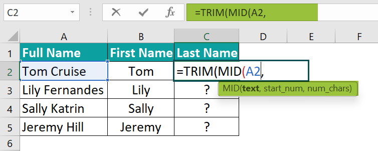
Step 10: Now, enter the value for the start_num argument and the SEARCH formula for extracting the last name.

Step 11: The value entered for the num_chars argument is the LEN excel formula as we are extracting the Last name.
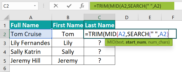
Step 12: So, the entered complete formula in cell C2 for extracting the last name is =TRIM(MID(A2,SEARCH(“ ”,A2),LEN(A2)))
Press Enter key.
The result is returned as Cruise.
Step 13: Drag the cursor to cell C5;
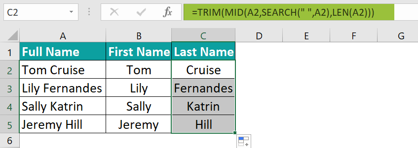
Likewise, we can use MID Function to extract values.
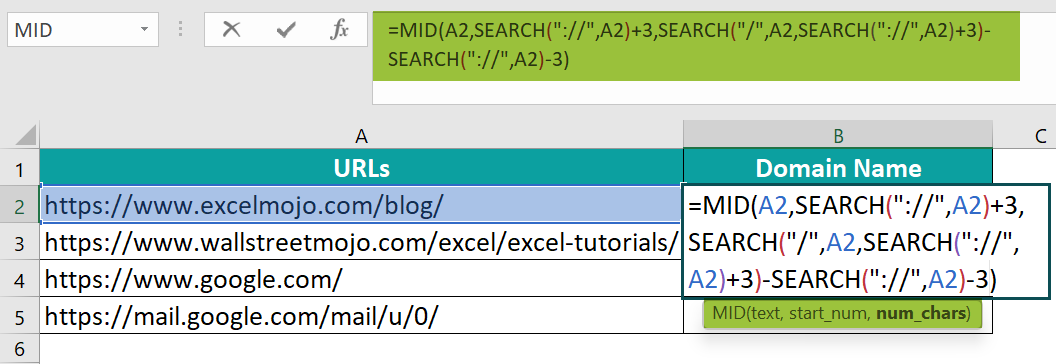
Example #2 – Find Out The Domain Name From The Web URLs
The below table shows the Web URLs in column A. We need to use the following steps to find the domain name from the table array using MID Excel Function.
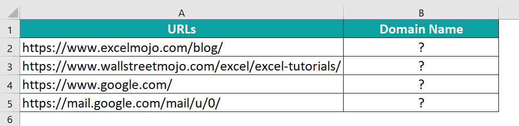
The steps to extract the text from the string by the MID in Excel are as follows:
Step 1: To begin with, select the column where we will enter the formula and calculate the result. The selected column, in this case, is column B.
Step 2: Next, enter the MID Excel formula in cell B2 for extracting the domain name.
Step 3: The complete formula in cell B2 for extracting the domain name is =MID(A2,SEARCH(“://”,A2)+3,SEARCH(“/”,A2,SEARCH(“://”,A2)+3)-SEARCH(“://”,A2)-3).
Step 4: The result is returned as www.excelmojo.com in cell B2.

Step 5: Now, drag the cursor to cell B5; all the domain name from the data is extracted in column B.
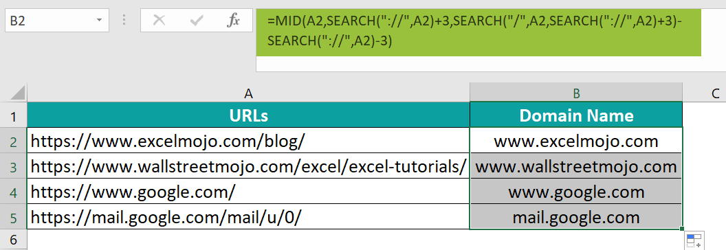
Similarly, we can use MID function to find the values.
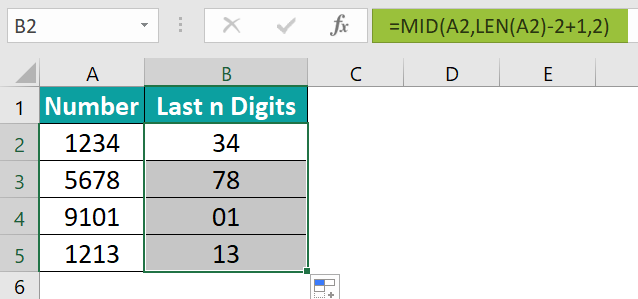
The following table shows numbers in column A. We need to extract the last n digits from the given data using MID Excel function.

The steps to extract the text from the string by the MID Excel function are as follows:
Step 1: First, select the column where we will enter the formula and calculate the result. The selected column, in this case, is column B.
Step 2: Next, enter the MID formula in cell B2 for extracting the Last n Digits.
Step 3: So, the complete formula in cell B2 for extracting the Last n Digits is =MID(A2,LEN(A2)-2+1,2).
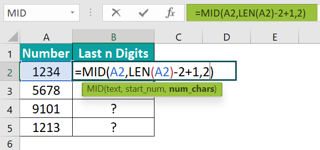
Step 4: The function has returned the result as 34 in cell B2.
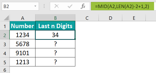
Step 5: Next, press Enter and drag the cursor to cell B5;
Likewise, we can use MID excel function to obtain the values.
Example #4 – MID Function With Arrays
The following table shows input values of fruits in column A. We need to extract the text from the table array using MID Excel function.
The steps to extract the text from the string by the MID in Excel are as follows:
Step 1: First, select the column where we will enter the formula and calculate the result. The selected column, in this case, is column B.
Step 2: Next, enter the MID formula in cell B2 for extracting the data from the array.
Step 3: Then, enter the value for the text argument as A2:A5.

Step 4: Similarly, enter the value for the start_num argument as 1.

Step 5: The value entered for the num_chars argument is the SEARCH formula as we extract the text.
Step 6: The entered complete formula in cell B2 for extracting is =MID(A2:A5,1,SEARCH(“ ”,A2:A5)).

We can see that the function has returned the value in B2.

Step 7: Drag the cursor to cell B5;
Similarly, we can use MID Excel function to find values.
Things To Remember
- The MID Excel function returns the middle or central characters in the data.
- All the arguments in MID Excel formula are mandatory.
- The function extracts the characters from any side of a specified text.
- It extracts text from inside a text string based on location and length.
- The MID function returns empty text if the start_num is greater than the length of a string.
- The “#VALUE!” error occurs if the value of the num_chars argument is less than 0 or if the value of the start_num argument is less than 1.
Frequently Asked Questions (FAQs)
1. What does the MID function do in Excel?
The MID function extracts the substring from the main string.
The syntax of MID is
=MID(text,start_num,num_chars)
For example, the below table shows the value in cell A2. We need to apply MID Excel function to detect the output.
The MID formula is entered in cell B2; the complete formula is =MID(A2,4,3),and the result is returned as 456.
Likewise, we can apply MID Excel function to obtain values.
2. When to use the MID Excel function?
The MID Excel function is used when we want to extract a small amount of data from huge data. That is when we want to fetch the text or number from a string or bunch of numbers.
3. Why does the MID function not work in Excel?
The MID function does not work in Excel due to two reasons;
1. If the value is equal to ‘0,’ the MID function will return a blank cell.
2. If the value is less than ‘0,’ the MID function will return “#VALUE!”.
Download Template
This article must help understand MID in Excel with its formula and examples. You can download the template here to use it instantly.
Recommended Articles
This has been a guide to MID Excel Function. Here we learn how MID() works with SEARCH, TRIM and LEN functions, examples & downloadable excel template. You can learn more from the following articles –
- NOT Excel Function
- TEXT Function In Excel
- Wrap Text In Excel
MID Function in Excel (Table of Contents)
- MID in Excel
- How to Use MID Function in Excel?
MID in Excel
The MID function works in the same way as the Right and Left functions do. It is all up to us what portion of the middle text we want to extract. For example, a cell contains FIRST, then using the Mid function there, we can select the character position from which we want to extract the text and the number of characters till we want. If we want from 2 positions to the next 3 characters, then we will be getting IRS as output.
For Example:
MID (“Bangalore is the Capital of Karnataka”, 18, 7) in this formula MID function will return from the 18th character it will return 7 characters, i.e. “Capital”.
The MID function is also available in VBA too. We will discuss that at the end of this article.
MID Formula in Excel:
Below is the MID Formula in Excel.
Explanation of MID Formula in Excel:
MID formula has three compulsory parameters: i.e.text, start_num, num_chars.
- text: From the text that you want to extract specified characters.
- start_num: Starting position of the middle string.
- [num_chars]: The number of characters you want to extract from the start-num.
Usually, the MID function in Excel is used alongside other text functions like SEARCH, REPLACE, LEN, FIND, LEFT, etc.
How to Use MID Function in Excel?
MID function in Excel is very simple and easy to use. Let understand the working of MID function in Excel by some MID Formula example. The MID function can be used as a worksheet function and as a VBA function.
You can download this MID Function Excel Template here – MID Function Excel Template
Example #1
In this MID Formula in Excel example, we are extracting the substring from the given text string by using the MID formula.
From the above table extract, characters from the 4th character extract 6 characters.
So the result will be :
Example #2
Using the MID function, we can extract First Name & Last Name. Look at the below example where we have full names from A2 to A15.
From the above table, extract first names for all the names.
Result is :
Part 1: This part determines the desired text that you want to extract the characters.
Part 2: This determines the starting position of the character.
Part 3: The SEARCH function looks for the first space (“ “) in the text and determines the placing of the space.
Here the SEARCH formula returns 5 for the first name that means space is the 5th character in the above text. So now MID function extracts 5 characters starting from 1st.
So the result will be :
NOTE: Space is also considered as one character.
Example #3
Below is the flight number list, and we need to extract the characters starting from Y till you find “ – “
Look at the above example where the letters are in bold we need to extract. It looks like one heck of a task, Isn’t it?. However, we can do this by using MID alongside SEARCH or FIND functions. One common thing is all the bold letters are starting with Y, and it has 6 characters in total.
A SEARCH function will determine the starting character to extract, and from the starting point, we need to extract 6 characters.
So the Result is :
Example #4
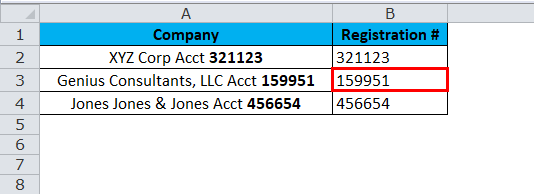
Below is the list of companies alongside their registration number. The task is to extract only the registration number from the list.
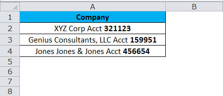
Closely look at the above list; one common thing before the registration number is the word Acct. This will be our key point to determine the starting point. In the previous example, we have used SEARCH this time to look at the FIND function.
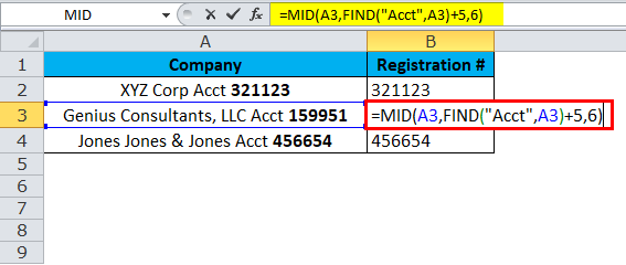
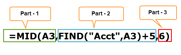
Part 1: This part determines the desired text that you want to extract the characters.
Part 2: The FIND function first looks for the word “Acct” in the text, and from there, we need to add 5 more characters to the list, and that determines the starting position of the character.
We need to add 5 that from Acct to registration number; it is 5 characters, including space.
Part 3: Number of characters we need to extract.
So the result will be :
Example #5
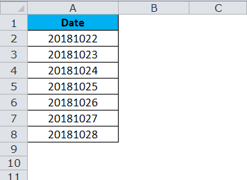
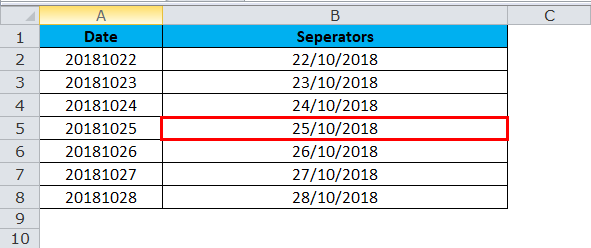
Now we will look at the combination of RIGHT, LEFT & MID function in one example. We need to concatenate forward-slash (/) to separate Year, month & day.
Look at the below example where we have dates but no separators for a year, month and day.
Now, we need to insert separators for the year, month, and day.
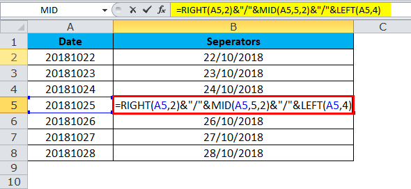
Firstly RIGHT function extracts 2 characters from the right and inserts one forward-slash (/), i.e. 25/
Now, we need to insert separators for the year, month, and day.
The second part is MID function extracts 2 characters starting from the 5th character and insert one forward-slash (/)
i.e. 25/10/
The final part is LEFT function extracts 4 characters from the left-hand side and insert one forward-slash (/)
i.e. 25/10/2018
So the result will be :
VBA Code to use MID Function
Like in Excel, we can use the MID function in VBA code also. The below code illustrates the usage of the MID function in VBA macros.
Sub MID_Function_Example
Dim Middle_String as string
Middle_String = Mid (“Excel can do wonders”, 14, 7)
Msgbox Middle_String
End Sub
If you run the above code message box will display wonders as your result.
Things to Remember
- Number formatting is not part of a string and will not be extracted or counted.
- This is designed to extract the characters from any side of a specified text.
- If the user does not specify the last parameter, it will take 0 as by default.
- Num_chars must be greater than or equal to zero. If it is a negative number, it will throw the error as #VALUE.
- In the case of complex data sets, you need to use other text functions like SEARCH, FIND Num_chars parameter.
- Use the MID function when you want to extract text from inside a text string, based on location and length.
- The MID function returns empty text if the start_num is greater than the length of a string.
Recommended Articles
This has been a guide to MID in Excel. Here we discuss the MID Formula in Excel and how to use MID Function in Excel along with practical examples and downloadable excel templates. You can also go through our other suggested articles –
- Uses of AND Function in Excel
- Best Examples of COLUMN Function in Excel
- LOOKUP Function in Excel
- Amazing uses of FV Function in Excel
- How to Use MID Function in VBA?
How to Use Excel > Excel Functions > Excel MID Function
How to Use the Excel MID Function
Table of contents :
- What is the Excel MID Function?
- MID Syntax
- How to Use MID Function in Excel
- MID Example

What is the Excel MID Function?
The excel MID function extracts a certain number of texts from the specified position.
The MID function acts like the LEFT function if it takes characters from the first position or works like the RIGHT function if the number of characters taken reaches the end of the text.
MID Syntax
MID(text, start_num, num_chars)
text, required, the text containing the characters to extract from.
start_num, required, the first character position to extract.
num_char, required, the number of characters to extract.
How to Use MID Function in Excel
The following is an example of the MID function usage and the results.

MID Function #1
=MID(A2,12,5)
You got nothing it start_num argument greater then text length.
MID Function #2
=MID(A3,8,1000)
If num_char argument exceeds the text length, whatever the number you get the characters up to the end of the text.
MID Function #3
=MID(A4,0,6)
#VALUE! error appears if the start_num argument is smaller than 1, it could be 0 (zero) or a negative number.
MID Function #4
=MID(A5,1,6)
The MID function returns the same value as the LEFT function if start_num argument is equal to 1.
The MID Function #4 result is the same as the LEFT(A5,6) formula.
MID Function #5
=MID(A6,8,4)
The results of the MID function and the RIGHT function are the same if the num_char argument plus start_num argument is equal to the text length.
The MID function #5 result is the same as the RIGHT(A6,4) formula.
MID Function #6
=MID(A7,2,2)
The MID function can extract from a number too.
MID Function #7
=MID(A8,2,2)
Alphanumeric is not a problem for the MID function, because alphanumeric is a text.
MID Function #8
=MID(A9,2,2)
The MID function returns the same results for numbers 123456 and “Wednesday, January 3, 2238”. Why? Because Excel stores date in an integer number. “Wednesday, January 3, 2238” is the result of “Format cells” menu. The real value is an integer number 123456.
The MID function extracts the number but ignores the cell format.
MID Function #9
=MID(A10,2,2)
Why are the results of MID Function #9 and #10 not the same? Because cell A9 contains a date and cell A10 contains a text.
“Wednesday, January 3, 2238” in cell A9 is the result of the format cell menu while in cell A10 is the real value.
MID Function #10
=MID(A11,2,4)
Just like integer numbers, the MID function can extract decimal numbers and assuming decimal separators as one character.
MID Function #11
=MID(A12,2,4)
The results are like MID Function #10. Excel stores date value in integer number, while for time value excel stores as a decimal number.
If you format 2:57:46 AM to number-general the result is 0.12345.
MID Example
Another article using or explain about MID Function
Another Text Function
Another article about Text Function