
Excel is an electronic spreadsheet program that is used for storing, organizing, and manipulating data.
The information we’ve prepared refers to Microsoft Excel in general and is not limited to any specific version of the program.
What Excel Is Used For
Electronic spreadsheet programs were originally based on paper spreadsheets used for accounting. As such, the basic layout of computerized spreadsheets is the same as the paper ones. Related data is stored in tables — which are a collection of small rectangular boxes or cells organized into rows and columns.
All versions of Excel and other spreadsheet programs can store several spreadsheet pages in a single computer file. The saved computer file is often referred to as a workbook and each page in the workbook is a separate worksheet.
Spreadsheet Cells and Cell References
When you look at the Excel screen — or any other spreadsheet screen — you see a rectangular table or grid of rows and columns.
In newer versions of Excel, each worksheet contains roughly a million rows and more than 16,000 columns, which necessitates an addressing scheme in order to keep track of where data is located.
The horizontal rows are identified by numbers (1, 2, 3) and the vertical columns by letters of the alphabet (A, B, C). For columns beyond 26, columns are identified by two or more letters such as AA, AB, AC or AAA, AAB, etc.
The intersection point between a column and a row is the small rectangular box known as a cell. The cell is the basic unit for storing data in the worksheet, and because each worksheet contains millions of these cells, each one is identified by its cell reference.
A cell reference is a combination of the column letter and the row number such as A3, B6, and AA345. In these cell references, the column letter is always listed first.
Data Types, Formulas, and Functions
The types of data that a cell can hold include:
- Numbers
- Text
- Dates and times
- Boolean values
- Formulas
Formulas are used for calculations — usually incorporating data contained in other cells. These cells, however, may be located on different worksheets or in different workbooks.
Creating a formula starts by entering the equal sign in the cell where you want the answer displayed. Formulas can also include cell references to the location of data and one or more spreadsheet functions.
Functions in Excel and other electronic spreadsheets are built-in formulas that are designed to simplify carrying out a wide range of calculations – from common operations such as entering the date or time to more complex ones such as finding specific information located in large tables of data.
Excel and Financial Data
Spreadsheets are often used to store financial data. Formulas and functions that are used on this type of data include:
- Performing basic mathematical operations such as summing columns or rows of numbers
- Finding values such as profit or loss
- Calculating repayment plans for loans or mortgages
- Finding the average, maximum, minimum and other statistical values in a specified range of data
- Carrying out What-If analysis on data, where variables are modified one at a time to see how the change affects other data, such as expenses and profits
Excel’s Other Uses
Other common operations that Excel can be used for include:
- Graphing or charting data to assist users in identifying data trends
- Formatting data to make important data easy to find and understand
- Printing data and charts for use in reports
- Sorting and filtering data to find specific information
- Linking worksheet data and charts for use in other programs such as Microsoft PowerPoint and Word
- Importing data from database programs for analysis
Spreadsheets were the original «killer apps» for personal computers because of their ability to compile and make sense of information. Early spreadsheet programs such as VisiCalc and Lotus 1-2-3 were largely responsible for the growth in popularity of computers like the Apple II and the IBM PC as a business tool.
Excel Alternatives
Other current spreadsheet programs that are available for use include:
- Google Sheets: A free, web-based spreadsheet program
- Excel Online: A free, scaled-down, web-based version of Excel
- Open Office Calc: A free, downloadable spreadsheet program.
Thanks for letting us know!
Get the Latest Tech News Delivered Every Day
Subscribe
Data is the most consistent raw material that was, is, and will be required in every era and the most popular tool that is used by almost everyone in the world to manage data is undoubtedly Microsoft Excel. Excel is used by almost every organization and with so much popularity and importance, it is certain that every individual must have knowledge of Excel. In case you don’t have your hands on it yet, don’t worry because this Excel tutorial will guide you through all that you need to know.
Here is a glimpse of all the topics that are discussed over here:
- What is Excel?
- How to launch Excel?
- Screen Options
- Backstage View
- Workbooks and Worksheets
- Editing Worksheets
- Formatting MS Excel Worksheets
- MS Excel Formulas
- Functions
What is Excel?
Microsoft Excel is a spreadsheet (computer application that allows storage of data in a tabular form) developed by Microsoft. It can be used on Windows, macOS, IOS, and Android platforms. Some of its features include:
- Graphing tools
- Functions (Count, sum, text, date and time, financial, etc)
- Data Analysis (Filters, charts, tables, etc)
- Visual Basic for Application (VBA)
- Contains 300 examples for you
- Workbooks and worksheets
- Data Validation, etc
How to launch Excel?
Follow the steps given below to launch Excel:
- Download MS Office from the official website
- In the search bar, type MS Office and select MS Excel from the same
Once this is done, you will see the following screen:
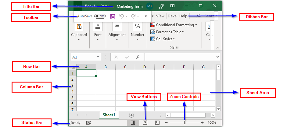
Screen Options:
Title Bar:
It displays the title of the sheet and appears right in the middle at the top of the Excel window.
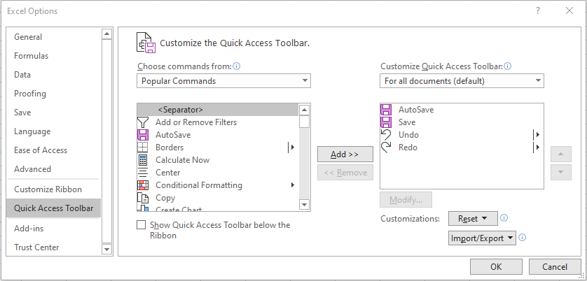
Quick Access Toolbar:
This toolbar consists of all commonly used Excel commands. In case you want to add some command that you use frequently to this toolbar, you can do it easily by customizing the quick access toolbar. To do that, right-click on it and select the option “Customize Quick Access Toolbar”. You will see the following window from where you can choose the appropriate commands that you would like to add.
Ribbon:
The ribbon tab consists of the File, Home, Insert, Page Layout, View, etc tabs. The default tab that is selected by Excel is the Home tab. Just like the Quick Access Toolbar, you can also customize the Ribbon tab.
In order to customize the Ribbon tab, right-click anywhere on it and select the option “Customize the Ribbon”. You will see the following dialog box:
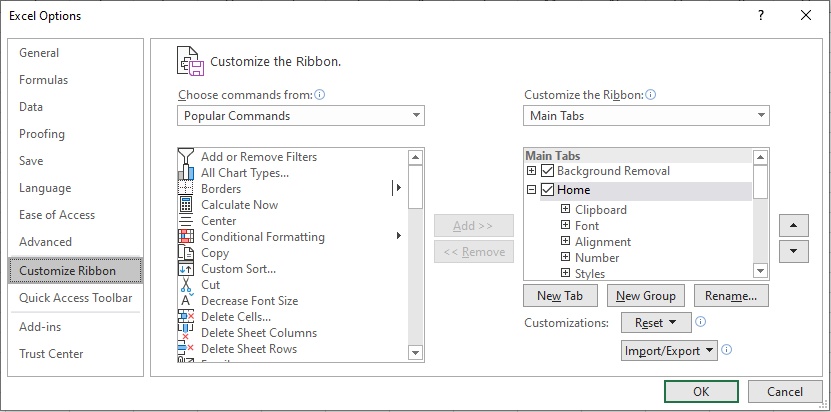
From here, you can select any tab that you want to add to the Ribbon bar according to your preference.
The Ribbon tab options are tailored into three components i.e Tabs, Groups and Commands. Tabs basically appear right on the top consisting of Home, Insert, file, etc. Groups consist of all related commands such as the font commands, insert commands, etc. Commands appear individually.
Zoom Control:
It allows you to zoom-in and zoom-out the sheet as and when required. To do this, you will just need to drag the slider towards the left side or the right side to zoom-in and zoom-out respectively.
View Buttons:
Consists of three options namely, the Normal Layout View, Page Layout View, and the Page Break View. Normal Layout View displays the sheet in a normal view. Page Layout View allows you to see the page just like it would appear when you take a print out of it. The Page Break View basically shows where the page is going to break when you print it.
Sheet Area:
This is the area wherein the data will be inserted. The flashing vertical bar or the insertion point indicates the position of data insertion.
Row Bar:
The Row bar shows the row numbers. It starts at 1 and the upper limit is 1,048,576 rows.
Column Bar:
The Column bar shows the columns in the A-Z order. It starts at A and goes on till Z following which, it goes on as AA, AB, etc. The upper limit for columns is 16,384.
Status Bar:
It is used to display the current status of the cell that is active in the sheet. There are four states namely Ready, Edit, Enter, and Point.
Ready, as the name suggests, is used to indicate that the worksheet can accept the user’s input.
Edit status indicates that the cell is in the editing-mode. In order to edit data of a cell, you can simply double click on that cell and enter the desired data.
Enter mode is enabled when the user starts to enter the data in the cell that is selected for editing.
Point mode is enabled when a formula is being entered into a cell with reference to the data present in some other cell.
Backstage View:
The Backstage view is the central managing place for all your Excel sheets. From here, you can create, save, open print or share your worksheets. To go to the Backstage, simply click on File and you will see a column with a number of options which are described in the following table:
|
Option |
Description |
|
New |
Used to open a new Excel sheet |
|
Info |
Gives information about the current worksheet |
|
Open |
In order to open some sheets created earlier, you can use Open |
|
Close |
Closes the open sheet |
|
Recent |
Displays all the recently opened Excel sheets |
|
Share |
Allows you to share the worksheet |
|
Save |
To save the current sheet as it is, choose Save |
|
Save As |
When you have to rename and select a particular file location for your sheet, you can use Save As |
|
|
USed to print the sheet |
|
Export |
Allows you to create a PDF or XPS document for your sheet |
|
Account |
Contains all the account holders details |
|
Options |
Shows all Excel options |
Workbooks and Worksheets:
Workbook:
Refers to your Excel file itself. When you open the Excel app, click on the Blank workbook option to create a new Workbook.
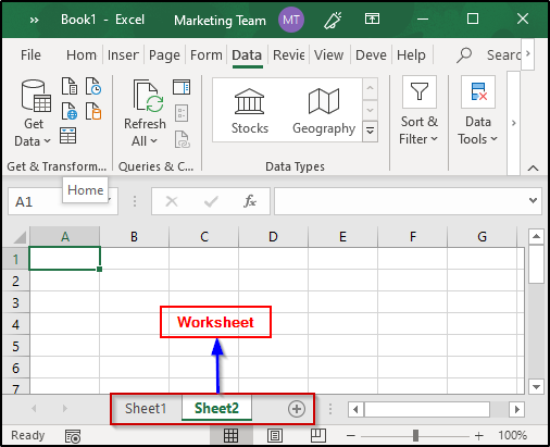
Worksheets:
Refers to a collection of cells wherein you manage your data. Each Excel workbook can have multiple worksheets. These sheets will be displayed towards the bottom of the window, with their respective names as shown in the image below.
Working with the Excel Worksheets:
Entering the Data:
As mentioned earlier, the data is entered into the Sheet Area and the flashing vertical bar represents the cell and the place where your data will be entered in that cell. If you wish to choose some particular cell, just left-click on that cell and then double-click on it to enable the Enter mode. You can also Move around using the keyboard’s arrow keys.
Saving a new Workbook:
To save your worksheet, click on the File tab and then select the Save As option. Select the appropriate folder where you would like to save the sheet and save it with an appropriate name. The default format in which an Excel file will be saved is .xlsx format.
In case you make changes to an existing file, you can just press Ctrl+S or open the File tab and select Save option. Excel also provides the Floppy Icon in the Quick Access toolbar to help you save your worksheet easily.
Creating a new Worksheet:
To create a new Worksheet, click on the + icon present next to the current Worksheet as shown in the image below:

You can also right-click on the Worksheet and select the Insert option to create a new Worksheet. Excel also provides a shortcut to create a new Worksheet i.e using Shift+F11.
Moving and Copying a Worksheet:
In case you have a Worksheet and you want to create another copy of it, you can do as follows:
- Right-click on the sheet that you desire to copy
- Select the ‘Move or Copy’ option


A dialog box will appear where you have the options to move the sheet at the required position and at the end of that dialog box, you will see an option as ‘Create a copy’. By checking that box, you will be able to create a copy of an existing sheet.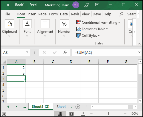
You can also left-click on the sheet and drag it to the required position in order to move the sheet. To rename the file, double-click on the desired file and rename it.
Hiding and Deleting Worksheets:
In order to hide a worksheet, right-click on the name of that sheet and select the Hide option. Conversely, if you want to undo this, right-click on any of the sheet names and select Unhide option. You will see a dialog box that contains all the hidden sheets, select the sheet that you want to unhide and click on OK.
To delete a sheet, right-click on the sheet name and select the Delete option. In case the sheet is empty, it will be deleted or else you will see a dialog box warning you that you might lose the data stored in that particular sheet.
Opening and Closing a Worksheet:
To close a Workbook, click on the File tab, and then select the Close option. You will see a dialog box asking you to optionally save the changes that have made to the Workbook in the desired directory.
To open a previously created Workbook, click on the File tab and select the Open option. You will see all the worksheets that have created previously when you select Open. left-click on the file that you intend to open.
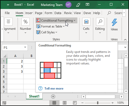
Excel Context Help:
Excel has a very special feature called the context help feature that provides appropriate information about the Excel commands in order to educate the user about its working as shown in the image below:
Editing the Worksheets:
The total number of cells present in an excel sheet is 16,384 x 1,048,576. The type of data i.e entered can be in any form such as textual, numerical or formulae.
Inserting, Selecting, Moving and Deleting Data:
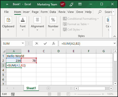
Inserting Data:
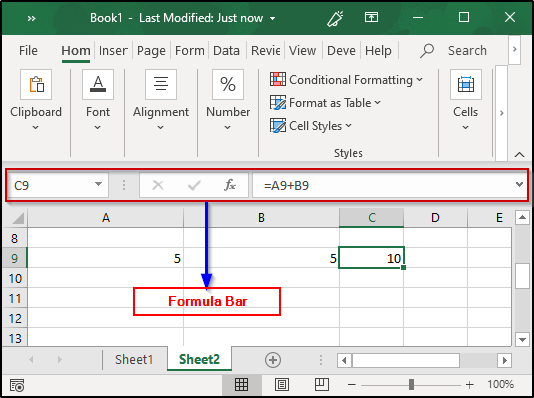
In order to enter the data, simply select the cell wherein you intend to insert the data and type the same. In case of formulas, you will need to enter them either directly in the cell or in the formula bar that is provided on top as shown in the image below:
Selecting Data:
there are two ways to select Excel data. The first and simplest way is to make use of the mouse. Just click on the required and cell and double click on it. Also, in case you want to select a complete section of data entries, hold left-click and drag it down till that cell which you intend to select. You can also hold the Ctrl button and left-click on random cells to select them.
The method is to use the Go To dialog box. To activate this box, you can either click on the Home tab and select the Find and Select option or simply click Ctrl+G. You will see a dialog box appearing that will have an option “Special”. Click on that option and you will see another dialog box as shown in the image below:
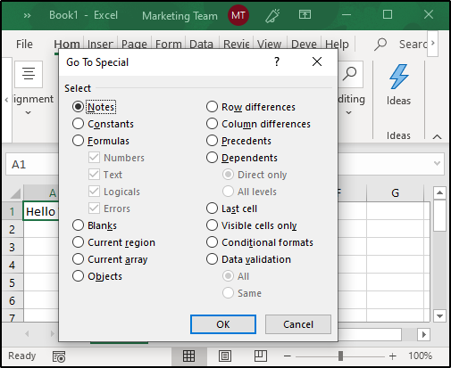
From here, check the appropriate region that you want to select and click on OK. Once this is done, you will see that the entire region of your choice has been selected.
Deleting Data:
In order to delete some data, you can use the following techniques:
- Click on the desired cell and highlight the data that you want to delete. Then press Delete button from the keyboard
- Select the cell or cells whose data is to be deleted and hit right-click. Then select the Delete option
- You can also click on the row number or column header to delete some entire row or column
Moving Data:
Excel also allows you to move your data easily to the desired location. You can do this in just two simple steps:
- Select the entire region that you want to move and then hit right-click
- Click on “Cut” and select the first cell where you want your data to be positioned and paste it using the “Paste” option
Copy, Paste, Find and Replace:
Copy and Paste:
If you want to Copy and Paste data in Excel, you can do it in the following ways:
- Select the region that you want to copy
- Right-click and select Copy option or press Ctrl+C
- Select the first cell where you want to copy it
- Hit right-click and click on the Paste option or just press Ctrl+V
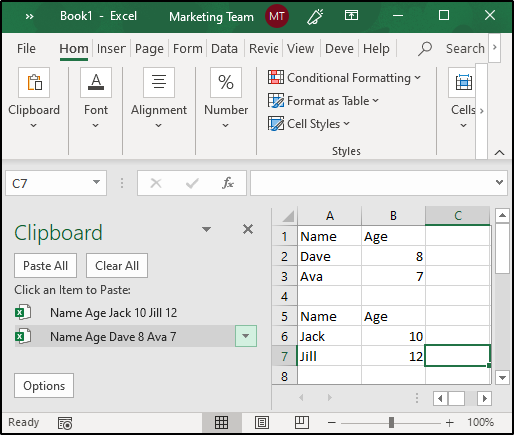
Excel also provides a Clipboard that will hold all the data that you have copied. In case you want to paste any of that data, simply select it from the Clipboard and choose the paste option as shown below:
Find and Replace:
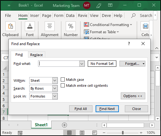
To Find and Replace data, you can either select the Find & Replace option from the Home tab or simply press Ctrl+F You will a dialog box that will have all the related options to find and replace the require data.
Special Symbols:
In case you need to enter a symbol that is not present on the keyboard, you can make use of the Special Symbols provided in Excel where you will find Equations and Symbols. In order to select these Symbols, click on the Insert tab and select Symbols option. You will have two options namely Equation and Symbols as shown below:

If you select Equation, you will find a number equations such as the Area of a circle, the Binomial Theorem, Expansion of a Sum, etc. If you select the Symbol, you will see the following dialog box:
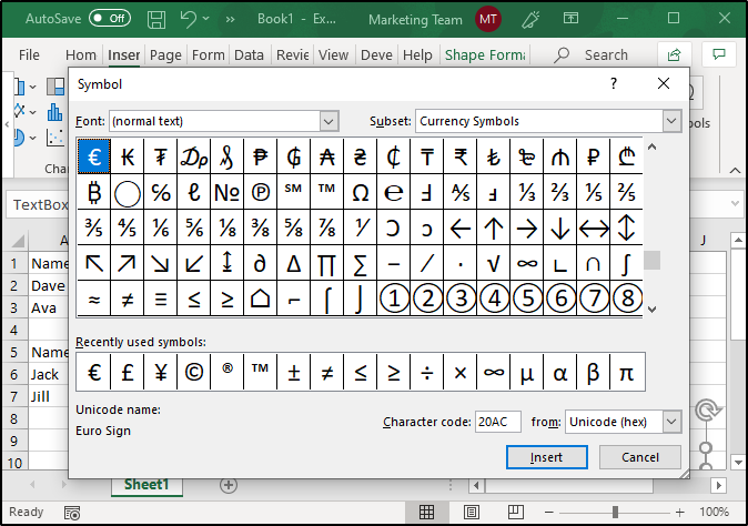
You can select any Symbol of your choice and click on the Insert option.
Commenting a Cell:
In order to give a clear description of the data, it is important to add comments. Excel allows you to add, modify and format comments.
Adding a Comment or a Note:
You can add comments and notes as follows:
- Right-click on the cell where you need to add a comment and select New Comment/ New Note
- Press Shift+F2 (New Note)
- Select the Review tab from the Ribbon and choose the New Comment Option
The comment dialog box will hold the user name of the system which can be replaced by the appropriate comments.
Editing Comments and Notes:
To edit a note, right-click on the cell that has the note and chose the Edit Note option and update it accordingly. In case you don’t need the note anymore, right-click on the cell containing it and choose the Delete Note option.
In case of a Comment, just select the cell containing the comment and it will open the comment dialog box from where you can edit or delete the comments. You can also reply to comments specified by other users working on that sheet.
Formatting the cells:
Cells of an Excel sheet can be formatted for the various types of data that they can hold. There are a number of ways to format the cells.
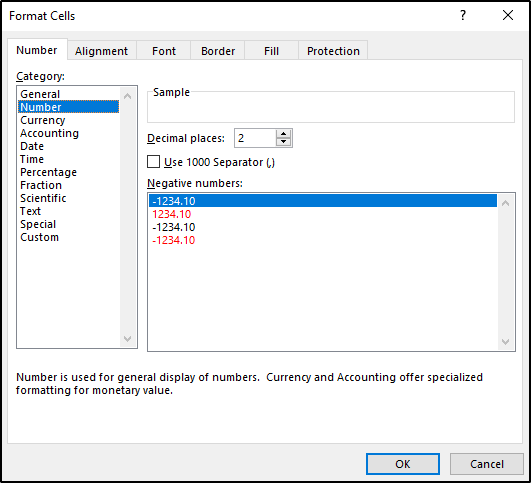
Setting the cell type:
The cells of an Excel sheet can be set to a particular type such as General, Number, Currency, Accounting, etc. To do this, right-click on the cell to which you intend to specify some particular type of data and then select Format cells option. You will see a dialog box as shown in the image below that will have a number of options to select from.
|
Type |
Description |
|
General |
No specific format |
|
Number |
General display of numbers |
|
Currency |
The cell will be displayed as a currency |
|
Accounting |
It is similar to currency type but used for accounts |
|
Date |
Allows various types of date formats |
|
Time |
Allows various types of time formats |
|
Percentage |
Cell displayed as a percentage |
|
Fraction |
The cell is displayed as a fraction |
|
Scientific |
Displays the cell in exponential form |
|
Text |
For Normal text data |
|
Special |
You can enter the special type of formats such as a phone number, ZIP, etc |
|
Custom |
Allows Custom formats |
Selecting Fonts and Decorating the data:
You can modify the font on an Excel sheet as follows:
- Click on the Home tab and from the Font group, select the required Font
- Right-click on the cell and select Format cells option. Then, from the dialog box, select the Font option and modify the text accordingly
In case you want to modify the look of the data, you can do so using the various options such as bold, italic, underline, etc that are present the same dialog box as shown in the image above or from the Home tab. You can select the effects options which are Strikethrough, Superscript, and Subscript.
Rotating the cells:
Cells of an Excel sheet can be rotated to any degree. To do this, click on the Orientation group tab present within Home and select the type of orientation you desire.
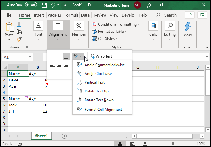
This can also be done from the Format cell dialog box by selecting the Alignment option. You also have options for aligning your data in various ways such as Top, Center, Justify, etc and you can change the direction as well using Context, Left-to-Right, and Right-to-Left options.
Merge and Shrink cells:
Merging:
The cells of an MS Excel sheet can be merged and unmerged as and when required. Keep the following points in mind when you merge cells of an Excel sheet:
- When you merge cells, you do not actually merge the data, but the cells are merged to behave as a single cell
- If you try to merge two or more cells that have data in them, only the data contained in the top-left cell will be preserved and the data of the other cells will be discarded
To merge cells, simply select all the cells you wish to merge and then select the Merge and Control option present in the Home tab or check the Merge cells option present in the Alignment window.
Shrink/ Wrap:
In case the cell holds a lot of data that starts to highlight other cells, you can use the Shrink to fit/ Wrap text options in order to reduce the size or align the text vertically.
Adding Borders and Shades:
In case you want to add borders and shades to a cell in your worksheet, select that cell and right-click over it and select the Format cells option.
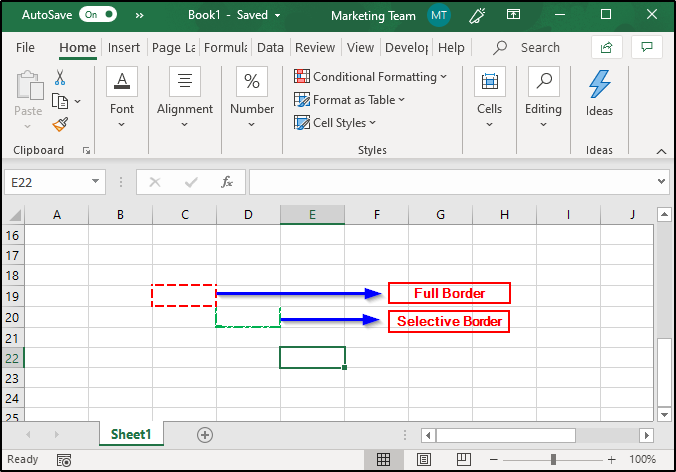
Borders:
To add borders, open the Border window from the Format cells window and then choose the type of border that you would like to add to that cell. You can also vary the thickness, color, etc.
Shades:
In case you want to add some shade to a cell, select that cell and then open the Fill pane from the Format cells window then choose the appropriate color of your choice.
Formatting MS Excel Worksheets:
Sheet Options:
Excel sheets provide a number of options for taking appropriate print outs. Using these options, you can selectively print your sheet in various ways. To open the sheet options pane, select Page Layout Group from the Home tab and open the Page Setup. Here, you will see a number of sheet options that are listed in the table below:
|
Option |
Description |
|
Print Area |
Sets the print area |
|
Print Titles |
Allows you to set the row and column titles to appear at the top and towards the left respectively |
|
Gridlines |
Gridlines will be added to the printout |
|
Black and White |
Print out is black and white or monochrome |
|
Draft Quality |
Prints the sheet using your printers Draft quality |
|
Row and Column Headings |
Allows you to print row and column headings |
|
Down, then over |
Prints the down pages first followed by the right pages |
|
Over, then down |
Prints the right pages first and then the down page |
Margins and Page Orientation:
Margins:
The unprinted regions along the top-down and left-right sides are referred to as margins. All MS Excel pages have a border and if you have selected some border for one page, then that border will be applied to all the pages i.e you can’t have different margins for each page. You can add margins as follows:
- From the Page Layout tab, select the Page Setup dialog and from there, you can either click on the Margins drop-down list or open the Margins window pane by maximizing the Page Setup window
- You can also add Margins while printing the page. In order to do that, select the File tab and click on Print. Here, you will be able to see a dropdown list having all the Margin options
Page Orientation:
Page Orientations refer to the format in which the sheet is printed i.e Portrait and Landscape. The Portrait orientation is default and prints the page taller than wide. On the other hand, the Landscape orientation prints the sheet wider than tall.
To select a particular type of page orientation, select the drop-down list from the Page Setup group or maximize the Page Setup window and choose the appropriate orientation. You can also change the page orientation while printing the MS Excel sheet just like how you did with Margins.
Headers and Footers:
Headers and Footers are used to provide some information at the top and at the bottom of the page. A new workbook does not have a Header or a Footer. In order to add it, you can open the Page Setup window and then open the Header/ Footer pane. Here, you will have a number of options to customize the Headers and Footers. If you want to preview the Header and Footers that you have added, click on the Print Preview option and you will be able to see the changes that you have made.
Page Breaks:
MS Excel allows you to precisely control what you want to print and what you want to omit. Using Page Breaks, you will be able to control the print of the page such as restrain from printing the first row of a table at the end of a page or printing the header of a new page at the end of the previous page. Using page breaks will allow you to print the sheet in the order of your preference. You can have both Horizontal as well as Vertical page breaks. To include this, select the row or column where you intend to include a page break and then from the Page Setup group, select the option Insert Page Break.
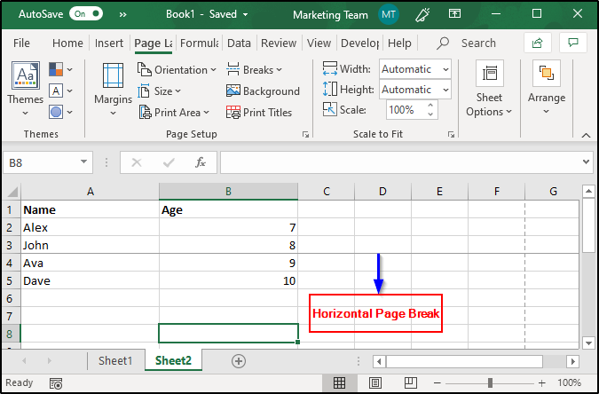
Horizontal Page Break:
To introduce a Horizontal Page Break, select the row where you want the page to break from. Take a look at the image below where I have introduced a Horizontal Page Break in order to print the row A4 on the next page.
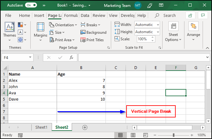
Vertical Page Break:
To introduce a Vertical Page Break, select the column where you want the page to break from. Take a look at the image below where I have introduced a Vertical Page Break.
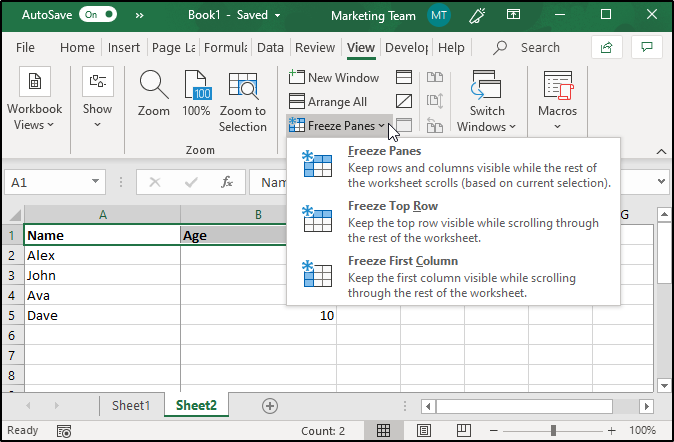
Freeing Panes:
MS Excel provides an option of freezing panes which will enable you to see the row and column headings even if you keep scrolling down the page. In order to Freeze Panes, you will have to:
- Select the Rows and Columns that you want to freeze
- Open the View tab and select the Freeze Pane group
- Here, you will have three options to freeze rows and columns
Conditional Formatting:
Conditional Formatting allows you to selectively format a section to hold values within some specified range. Values outside these ranges will be formatted automatically. This feature has a number of options which are listed in the table below:
|
Option |
Description |
|
Highlight Cells Rules |
Opens another list that defines the selected cells contain values, text or dates that are greater than, equal to, less than some particular value |
|
Top/ Bottom Rules |
Highlights the top/ bottom values, percents, as well as the upper and lower averages |
|
Data Bars |
Opens up a palette with differently colored data bars |
|
Color Scales |
Contains a color palette with two and three colored scales |
|
Icon Sets |
Contains different sets of icons |
|
New Rule |
Opens up a New Formatting rule dialog box for custom conditional formatting |
|
Clear Rules |
Allows you to remove the conditional formatting rules |
|
Manage Rules |
Conditional Formatting Rules Manager dialog box opens up from where you can add, delete or format rules according to your preference |
MS Excel Formulas:
Formulas are one of the most important features of an Excel sheet. A formula is basically an expression that can be entered into the cells and the output of that particular expression is displayed in that cell as the output. The formulas of an MS Excel sheet can be:
- Mathematical operators( +, -, *, etc)
- Example: =A1+B1; will add the values present in A1 and B1 and displays the output
- Values or text
- Example: 100*0.5 multiples 100 times 0.5; Takes only the values and returns the result)
- Cell reference
- EXAMPLE: =A1=B1; Compares the value of A1 with B1 and returns TRUE or FALSE
- Worksheet functions
- EXAMPLE: =SUM(A1: B1); Adds the values of A1 and B1
MS Excel allows you to enter formulas by a number of means such as:
- Creating Formulas
- Copying Formulas
- Formula References
- Functions
Creating Formulas:
For creating a formula, you will have to exclusively enter a formula in the formula bar of the sheet. The formula should always start with a “=” sign. You can manually build your formula by specifying cell addresses or just by pointing to the cell in the worksheet.
Copying Formulas:
You can copy Excel sheet formulas in case you have to calculate some common results. Excel automatically handles the task of copying formulas where ever similar ones are needed.
Relative Cell Addresses:
Like I have mentioned before, Excel automatically manages cell references of the original formula in order to match the position where it is copied. This task is accomplished through a system known as Relative Cell Addresses. Here, the copied formula will have modified row and column addresses that will suit its new position.
In order to copy a formula, select a cell that holds the original formula and drag it until the cell that you want to calculate the formula for. For example, in the previous example, I have calculated the sum of A9 and B9. Now, to calculate the sum of A10 and B10, all I have to do is, select C9 and drag it down to C10 as shown in the image below:
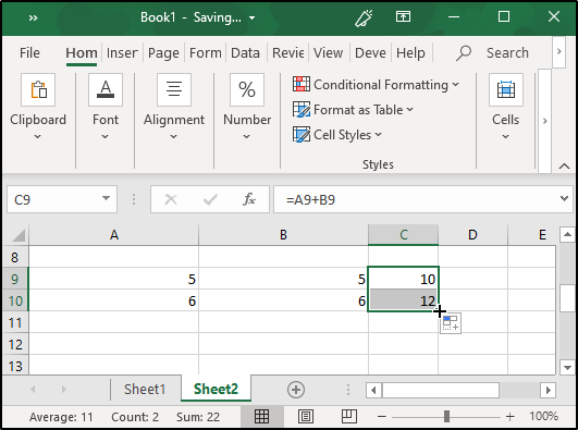
As you can see, the formula is copied without me having to exclusively specify the cell addresses.
Formula References:
Most of the Excel formulas are with reference to the cell or a range of cell addresses that enable you to work with the data dynamically. For example, if I change the value of any of the cells in the previous example, the result will be updated automatically.
This addressing can be of three types namely relative, absolute or mixed.
Relative Cell Address:
When you copy a formula, the row and column references change accordingly. This is because the cell references are actually the offsets from the current column or row.
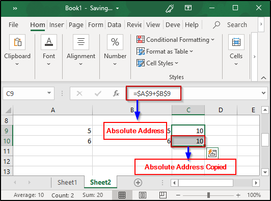
Absolute Cell Reference:
The row and column address do not get modified when copied as the reference points to the original cell itself. Absolute references are created using $ signs in the address preceding the column letter and the row number. For example, $A$9 is an absolute address.
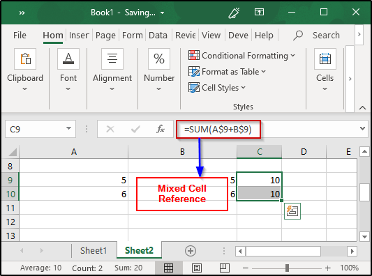
Mixed Cell Reference:
Here, either the cell or column is absolute and the other is relative. Take a look at the image below:
Functions:
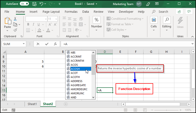
Functions available in MS Excel actually handle many of the formulas that you create. These functions actually define complex calculations that are difficult to manually define using just operators. Excel provides many functions and if you want some particular function, all you have to do is type in the first letter of that function in the formula bar and Excel will display a drop-down list holding all the functions that start with that letter. Not just this, hen you hover the mouse over these function names, Excel brilliantly gives a description about it. Take a look at the image below:
Built-in Functions:
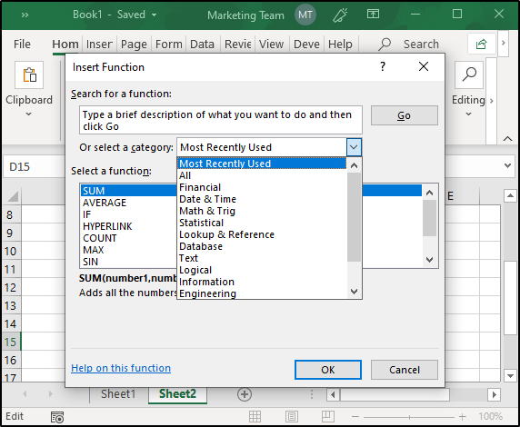
Excel provides a huge number of built-in functions that you can use in any of your formulas. to look out for all the functions, click on fx and then you will see a window opening that will have all Excel’s built-in functions. From here you can select any function based on the category to which it belongs.
Some of the most important built-in Excel Functions include If STATEMENTS, SUMIF, COUNTIF, VLOOKUP, HLOOKUP, CONCATENATE, MAX, MIN, etc.
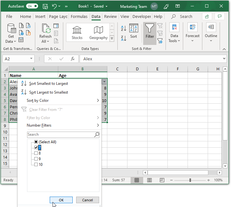
Data Filtering:
Filtering the data basically means to pull out data from those rows and columns that meet some specific conditions. In this case, the other rows or columns get hidden. For example, if you have a list of student Names with their Ages, and if you want to filter out only those students that are of 7 years, all you have to do is, select a specific range of cells and from the Data tab, click on the Filter command. Once this is done, you will be able to see a drop-down list as shown in the image below:
Advanced Tutorial:
Advanced Excel tutorial includes all the topics that will help you learn to manage real-time data using excel sheets. It includes using complex Excel functions, creating charts, filtering data, pivot charts and pivot tables, data charts and tables, etc.
This brings us to the end of this article on Excel Tutorial. I hope you are clear with all that has been shared with you. Make sure you practice as much as possible and revert your experience.
Also, If you’re looking to improve your abilities and learn more about Data Visualization to become certified as a Business Intelligence Professional. Go through our Tableau Training Course now to get all the information you should learn about this powerful software.
![]()
Download Article
![]()
Download Article
Are you new to Microsoft Excel and need to work on a spreadsheet? Excel is so overrun with useful and complicated features that it might seem impossible for a beginner to learn. But don’t worry—once you learn a few basic tricks, you’ll be entering, manipulating, calculating, and graphing data in no time! This wikiHow tutorial will introduce you to the most important features and functions you’ll need to know when starting out with Excel, from entering and sorting basic data to writing your first formulas.
Things You Should Know
- Use Quick Analysis in Excel to perform quick calculations and create helpful graphs without any prior Excel knowledge.
- Adding your data to a table makes it easy to sort and filter data by your preferred criteria.
- Even if you’re not a math person, you can use basic Excel math functions to add, subtract, find averages and more in seconds.
-

1
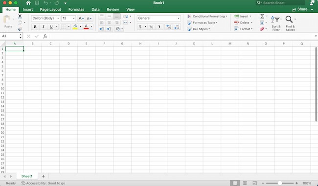
Create or open a workbook. When people refer to «Excel files,» they are referring to workbooks, which are files that contain one or more sheets of data on individual tabs. Each tab is called a worksheet or spreadsheet, both of which are used interchangeably. When you open Excel, you’ll be prompted to open or create a workbook.
- To start from scratch, click Blank workbook. Otherwise, you can open an existing workbook or create a new one from one of Excel’s helpful templates, such as those designed for budgeting.
-
2
Explore the worksheet. When you create a new blank workbook, you’ll have a single worksheet called Sheet1 (you’ll see that on the tab at the bottom) that contains a grid for your data. Worksheets are made of individual cells that are organized into columns and rows.
- Columns are vertical and labeled with letters, which appear above each column.
- Rows are horizontal and are labeled by numbers, which you’ll see running along the left side of the worksheet.
- Every cell has an address which contains its column letter and row number. For example, the top-left cell in your worksheet’s address is A1 because it’s in column A, row 1.
- A workbook can have multiple worksheets, all containing different sets of data. Each worksheet in your workbook has a name—you can rename a worksheet by right-clicking its tab and selecting Rename.
- To add another worksheet, just click the + next to the worksheet tab(s).
Advertisement
-
3
Save your workbook. Once you save your workbook once, Excel will automatically save any changes you make by default.[1]
This prevents you from accidentally losing data.- Click the File menu and select Save As.
- Choose a location to save the file, such as on your computer or in OneDrive.
- Type a name for your workbook. All workbooks will automatically inherit the the .XLSX file extension.
- Click Save.


Advertisement
-
1
Click a cell to select it. When you click a cell, it will highlight to indicate that it’s selected.
- When you type something into a cell, the input text is called a value. Entering data into Excel is as simple as typing values into each cell.
- When entering data, the first row of your worksheet (e.g., A1, B1, C1) is typically used as headers for each column. This is helpful when creating graphs or tables which require labels.
- For example, if you’re adding a list of dates in column A, you might click cell A1 and type Date into the cell as the column header.
-
2
Type a word or number into the cell. As you’re typing, you’ll see the letters and/or numbers appear in the cell, as well as in the formula bar at the top of the worksheet.
- When you start practicing more advanced Excel features like creating formulas, this bar will come in handy.
- You can also copy and paste text from other applications into your worksheet, tables from PDFs and the web.
-
3
Press ↵ Enter or ⏎ Return. This enters the data into the cell and moves to the next cell in the column.
-
4
Automatically fill columns based on existing data. Let’s say you want to make a list of consecutive dates or numbers. Or what if you want to fill a column with many of the same values that follow a pattern? As long as Excel can recognize some sort of pattern in your data, such as a particular order, you can use Autofill to automatically populate data into the rest of your column. Here’s a trick to see it in action.
- In a blank column, type 1 into the first cell, 2 into the second cell, and then 3 into the third cell.
- Hover your mouse cursor over the bottom-right corner of the last cell in your series—it will turn to a crosshair.
- Click and drag the crosshair down the column, then release the mouse button once you’ve gone down as far as you like. By default, this will fill the remaining cells with the value of the selected cell—at this point, you’ll probably have something like 1, 2, 3, 3, 3, 3, 3, 3.
- Click the small icon at the bottom-right corner of the filled data to open AutoFill options, and select Fill Series to automatically detect the series or pattern. Now you’ll have a list of consecutive numbers. Try this cool feature out with different patterns!
- Once you get the hang of AutoFill, you’ll have to try flash fill, which you can use to join two columns of data into a single merged column.
-
5
Adjust the column sizes so you can see all of the values. Sometimes typing long values into a cell hides the value and displays hash symbols ### instead of what you’ve typed. If you want to be able to see everything, you can snap the cell contents to the width of the widest cell. For example, let’s say we have some long values in column B:
- To expand the contents of column B, hover the cursor over the dividing line between the B and C at the top of the worksheet—once your cursor is right on the line, it will turn to two arrows pointing in either direction.[2]
- Click and drag the separator until the column is wide enough to accommodate your data, or just double-click the separator to instantly snap the column to the size of the widest value.
- To expand the contents of column B, hover the cursor over the dividing line between the B and C at the top of the worksheet—once your cursor is right on the line, it will turn to two arrows pointing in either direction.[2]
-
6
Wrap text in a cell. If your longer values are now awkwardly long, you can enable text wrapping in one or more cells. Just click a cell (or drag the mouse to select multiple cells), click the Home tab, and then click Wrap Text on the toolbar.
-
7
Edit a cell value. If you need to make a change to a cell, you can double-click the cell to activate the cursor, and then make any changes you need. When you’re finished, just press Enter or Return again.
- To delete the contents of a cell, click the cell once and press delete on your keyboard.
-
8
Apply styles to your data. Whether you want to highlight certain values with color so they stand out or just want to make your data look pretty, changing the colors of cells and their containing values is easy—especially if you’re used to Microsoft Word:
- Select a cell, column, row, or multiple cells at once.
- On the Home tab, click Cell Styles if you’d like to quickly apply quick color styles.
- If you’d rather use more custom options, right-click the selected cell(s) and select Format Cells. Then, use the colors on the Fill tab to customize the cell’s background, or the colors on the Font tab for value colors.
-
9
Apply number formatting to cells containing numbers. If you have data that contains numbers such as prices, measurements, dates, or times, you can apply number formatting to the data so it will display consistently.[3]
By default, the number format is General, which means numbers display exactly as you type them.- Select the cell you want to format. If you’re working with an entire column or row, you can just click the column letter or row number to select the whole thing.
- On the Home tab, click the drop-down menu at the top-center—it’ll say General by default, unless you selected cells that Excel recognizes as a different type of number like Currency or Time.
- Choose one of the formatting options in the list, such as Short Date or Percentage, or click More Number Formats at the bottom to expand all options (we recommend this!).
- If you selected More Number Formats, the Format Cells dialog will expand to the Number tab, where you’ll see several categories for number types.
- Select a category, such as Currency if working with money, or Date if working with dates. Then, choose your preferences, such as a currency symbol and/or decimal places.
- Click OK to apply your formatting.


Advertisement
-
1
Select all of the data you’ve entered so far. Adding your data to a table is the easiest way to work with and analyze data.[4]
Start by highlighting the values you’ve entered so far, including your column headers. Tables also make it easy to sort and filter your data based on values.- Tables traditionally apply different or alternating colors to every other row for easy viewing. Many table options also add borders between cells and/or columns and rows.
-
2
Click Format as Table. You’ll see this at the top-center part of the Home tab.[5]
-
3
Select a table style. Choose any of Excel’s default table styles to get started. You’ll see a small window titled «Create Table» once selected.
- Once you get the hang of tables, you can return here to customize your table further by selecting New Table Style.
-
4
Make sure «My table has headers» is selected and click OK. This tells Excel to turn your column headers into drop-down menus that you can easily sort and filter. Once you click OK, you’ll see that your data now has a color scheme and drop-down menus.
-
5
Click the drop-down menu at the top of a column. Now you’ll see options for sorting that column, as well as several options for filtering all of your data based on its values.
-
6
Choose which data to display based on values in this column. The simplest way to do this is to uncheck the values you don’t want to display—if you uncheck a particular date, for example, you’ll prevent rows that contain the selected date in from appearing in your data. You can also use Text Filters or Number Filters, depending on the type of data in the column:
- If you chose a numerical column, select Number Filters, then choose an option like Greater Than… or Does Not Equal to be extra specific about which values to hide.
- For text columns, you can choose Text Filters, where you can specify things like Begins with or Contains.
- You can also filter by cell color.
-
7
Click OK. Your data is now filtered based on your selections. You’ll also see a small funnel icon in the drop-down menu, which indicates that the data is filtering out certain values.
- To unfilter your data, click the funnel icon, click Clear filter from (column name), and then click OK.
- You can also filter columns that aren’t in tables. Just select a column and click Filter on the Data tab to add a drop-down to that column.
-
8
Sort your data in ascending or descending order. Click the drop-down arrow at the top of a column to view sorting options—these allow you to sort all of your data in order based on the current column.
- If you’re working with numbers, click Smallest to Largest to sort in ascending order, or Largest to Smallest for descending order.[6]
- If you’re working with text values, Sort A to Z will sort in ascending order, while Sort Z to A will sort in reverse.
- When it comes to sorting dates and times, Sort Oldest to Newest will sort with the earliest date at the top and the oldest date at the bottom, and Newest to Oldest displays the dates in descending order.
- When you sort a column, all other columns in the table adjust based on the sort.
- If you’re working with numbers, click Smallest to Largest to sort in ascending order, or Largest to Smallest for descending order.[6]


Advertisement
-
1
Select the data in your worksheet. Excel’s Quick Analysis feature is the easiest way to perform basic calculations (including totals, averages, and counts) and create meaningful tables or graphs without the need for advanced Excel knowledge.[7]
Use your mouse to select your data (including your column headers) to get started. -
2
Click the Quick Analysis icon. This is the small icon that pops up at the bottom-right corner of your selection. It looks like a window with some colored lines.
-
3
Select an analysis type. You’ll see several tabs running along the top of the window, each of which gives you different option for visualizing your data:
- For math calculations, click the Totals tab, where you can select Sum, Average, Count, %Total, or Running Total. You’ll be able to choose whether to display the results at the bottom of each column or to the right.
- To create a chart, click the Charts tab, then select a chart to visualize your data. Before you settle on a chart, just hover the cursor over each option to see a preview.
- To add quick chart data to individual cells, click the Sparklines tab and choose a format. Again, you can hover the cursor over each option to see a preview.
- To instantly apply conditional formatting (which is usually a little more complex in Excel) based on your data, use the Formatting tab. Here you can choose an option like Color or Data Bars, which apply colors to your data based on trends.


Advertisement
-
1
Quickly add data with AutoSum. AutoSum is a built-in Excel function that makes it easy to find the total of one or more columns in a few clicks. Functions or formulas that perform calculations and other tasks based on the values of cells. When you use a function to get something done, you’re creating a formula, which is like a math equation. If you have a column or row of numbers you want to add:
- Click the cell below the numbers you want to add (if a column) or to the right (if a row).[8]
- On the Home tab, click AutoSum toward the upper-right corner of the app. A formula beginning with =SUM(cell+cell) will appear in the field, and a dotted line will surround the numbers you’re adding.
- Press Enter or Return. You should now see the total of the numbers in the selected field. This is here because you created your first formula—which you didn’t have to write by hand!
- If you change any numbers in your data after using AutoSum, the AutoSum value will update automatically.
- Click the cell below the numbers you want to add (if a column) or to the right (if a row).[8]
-
2
Write a simple math formula. AutoSum is just the beginning—Excel is famous for its ability to do all sorts of simple and complex math calculations on data. Fortunately, you don’t have to be a math whiz to create simple formulas to create everyday math formulas, like adding, subtracting, and multiplying. Here’s some basic formulas to get you started:
-
Add: — Type =SUM(cell+cell) (e.g.,
=SUM(A3+B3)) to add two cells’ values together, or type =SUM(cell,cell,cell) (e.g.,=SUM(A2,B2,C2)) to add a series of cell values together.- If you want to add all of the numbers in a whole column (or in a section of a column), type =SUM(cell:cell) (e.g.,
=SUM(A1:A12)) into the cell you want to use to display the result.
- If you want to add all of the numbers in a whole column (or in a section of a column), type =SUM(cell:cell) (e.g.,
-
Subtract: Type =SUM(cell-cell) (e.g.,
=SUM(A3-B3)) to subtract one cell value from another cell’s value. -
Divide: Type =SUM(cell/cell) (e.g.,
=SUM(A6/C5)) to divide one cell’s value by another cell’s value. -
Multiply: Type =SUM(cell*cell) (e.g.,
=SUM(A2*A7)) to multiply two cell values together.
-
Add: — Type =SUM(cell+cell) (e.g.,


Advertisement
-
1
Select a cell for an advanced formula. What if you need to do something more complicated than just adding numbers? Even if you don’t know how to write formulas by hand, you can still create useful formulas that work with your data in various ways. Start by clicking the cell in which you want to display your formula.
-
2
Click the Formulas tab. It’s a tab at the top of the Excel window.
-
3
Explore the Function Library. Several function categories appear in the toolbar, such as Financial, Text, and Math & Trig. Click the options to check out the types of functions available, though they might not make a whole lot of sense just yet.
-
4
Click Insert Function. This option is in the far-left side of the Formulas toolbar. This opens the Insert Function window, which gives you a more detailed breakdown of each function.
-
5
Click a function to learn about it. You can type what you want to do (such as round), or choose a category to filter the list of functions. Then, click any function to read a description of how it works and view its syntax.
- For example, to select the formula for finding the tangent of an angle, you would scroll down and click the TAN option.
-
6
Select a function and click OK. This creates a formula based on the selected function.
-
7
Fill out the function’s formula. When prompted, type in the number or select a cell for which you want to use the formula.
- For example, if you select the TAN function, you’ll type in the number for which you want to find the tangent, or select the cell that contains that number.
- Depending on your selected function, you may need to click through a couple of on-screen prompts.
-
8
Press ↵ Enter or ⏎ Return to run the formula. Doing so applies your function and displays it in your selected cell.


Advertisement
-
1
Set up the chart’s data. If you’re creating a line graph or a bar graph, for example, you’ll want to use one column of cells for the horizontal axis and one column of cells for the vertical axis. The best way to do this is to place your data in a table.
- Typically speaking, the left column is used for the horizontal axis and the column immediately to the right of it represents the vertical axis.
-
2
Select the data in your table. Click and drag your mouse from the top-left cell of the data down to the bottom-right cell of the data.
-
3
Click the Insert tab. It’s a tab at the top of the Excel window.
-
4
Click Recommended Charts. You’ll find this option in the «Charts» section of the Insert toolbar. A window with different chart templates will appear.
-
5
Select a chart template. Click the chart template you want to use based on the type of data you’re working with. If you don’t see a chart type you like, click the All Charts tab to explore by category, such as Pie, Bar, and X Y Scatter.
-
6
Click OK. It’s at the bottom of the window. This creates your chart.
-
7
Use the Chart Design tab to customize your chart. Any time you click your chart, the Chart Design tab will appear at the top of Excel. You can adjust the chart style here, change colors, and add additional elements.
-
8
Double-click a chart element to manage it in the Format panel. When you double-click something on your chart, such as a value, line, or bar, you’ll see options you can edit in the panel on the right side of excel. Here you can change the axis labels, alignment, and legend data.


Advertisement
Add New Question
-
Question
How do you add a check mark or an X mark to a cell?

You can go into Insert, then Symbol, and choose the symbol you want. After that, you can just copy and paste the symbol from one cell to another.
-
Question
Can I add work sheets on Excel?
Yes. At the bottom left of the Excel you will see the list of sheets. To the left of those sheets you will find a «+» sign. Click on it.
-
Question
How do I move cell contents to another cell?
Highlight the cell, right-click, and click Copy. Click destination cell, right-click and Paste.
See more answers
Ask a Question
200 characters left
Include your email address to get a message when this question is answered.
Submit
Advertisement
Video
Thanks for submitting a tip for review!
References
About This Article
Article SummaryX
1. Purchase and install Microsoft Office.
2. Enter data into individual cells.
3. Format cells based on certain criteria.
4. Organize data into rows and columns.
5. Perform math operations using formulas.
6. Use the Formulas tab to find additional formulas.
7. Use data to create charts.
8. Import data from other sources.
Did this summary help you?
Thanks to all authors for creating a page that has been read 646,684 times.
Reader Success Stories
-

«I am applying for a job that requires comprehensive knowledge of Excel. Well, I don’t have it, but this article…» more
Is this article up to date?
Microsoft Excel know-how is so expected that it hardly warrants a line on a resume anymore. But how well do you really know how to use it?
Marketing is more data-driven than ever before. At any time you could be tracking growth rates, content analysis, or marketing ROI. You may know how to plug in numbers and add up cells in a column in Excel, but that’s not going to get you far when it comes to metrics reporting.
![Download 10 Excel Templates for Marketers [Free Kit]](https://no-cache.hubspot.com/cta/default/53/9ff7a4fe-5293-496c-acca-566bc6e73f42.png)
Do you want to understand what pivot tables are? Are you ready for your first VLOOKUP? Aspiring Excel wizard, read on or jump to the section that interests you most:
What is Microsoft Excel?
Microsoft Excel is a popular spreadsheet software program for business. It’s used for data entry and management, charts and graphs, and project management. You can format, organize, visualize, and calculate data with this tool.
How to Download Microsoft Excel
It’s easy to download Microsoft Excel. First, check to make sure that your PC or Mac meets Microsoft’s system requirements. Next, sign in and install Microsoft 365.
After you sign in, follow the steps for your account and computer system to download and launch the program.
For example, say you’re working on a Mac desktop. You’ll click on Launchpad or look in your applications folder. Then, click on the Excel icon to open the application.
Microsoft Excel Spreadsheet Basics
Sometimes, Excel seems too good to be true. Need to combine data in multiple cells? Excel can do it. Need to copy formatting across an array of cells? Excel can do that, too.
Let’s start this Excel guide with the basics. Once you have these functions down, you’ll be ready to tackle more pro Excel tips and advanced lessons.
Inserting Rows or Columns
As you work with data, you might find yourself needing to add more rows and columns. Doing this one at a time would be super tedious. Luckily, there’s an easier way.
To add multiple rows or columns in a spreadsheet, highlight the number of pre-existing rows or columns that you want to add. Then, right-click and select «Insert.»
In this example, I add three rows to the top of my spreadsheet.
Autofill
Autofill lets you quickly fill adjacent cells with several types of data, including values, series, and formulas.
There are many ways to deploy this feature, but the fill handle is among the easiest.
First, choose the cells you want to be the source. Next, find the fill handle in the lower-right corner of the cell. Then either drag the fill handle to cover the cells you want to fill or just double-click.
Filters
When you’re looking at large data sets, you usually don’t need to look at every row at the same time. Sometimes, you only want to look at data that fit into certain criteria. That’s where filters come in.
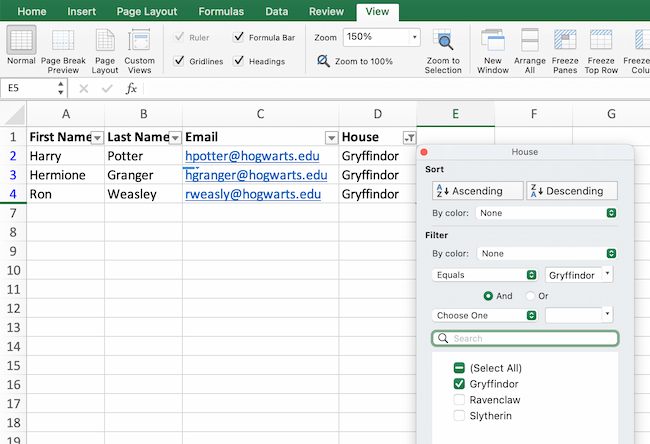
Filters allow you to pare down data to only see certain rows at one time. In Excel, you can add a filter to each column in your data. From there, you can choose which cells you want to view.
To add a filter, click the Data tab and select «Filter.» Next, click the arrow next to the column headers. This lets you choose whether you want to organize your data in ascending or descending order, as well as which rows you want to show.
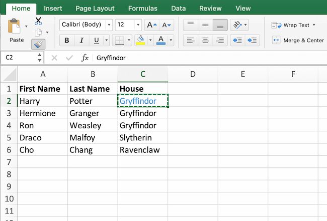
Let’s take a look at the Harry Potter example below. Say you only want to see the students in Gryffindor. By selecting the Gryffindor filter, the other rows disappear.
Pro tip: Start with a filtered view in your original spreadsheet. Then, copy and paste the values to another spreadsheet before you start analyzing.
Sort
Sometimes you’ll have a disorganized list of data. This is typical when you’re exporting lists, like marketing contacts or blog posts. Excel’s sort feature can help you alphabetize any list.
Click on the data in the column you want to sort. Then click on the «Data» tab in your toolbar and look for the «Sort» option on the left.
- If the «A» is on top of the «Z,» you can just click on that button once. Choosing A-Z means the list will sort in alphabetical order.
- If the «Z» is on top of the «A,» click the button twice. Z-A selection means the list will sort in reverse alphabetical order.
Remove Duplicates
Large datasets tend to have duplicate content. For example, you may have a list of different company contacts, but you only want to see the number of companies you have. In situations like this, removing duplicates comes in handy.
To remove duplicates, highlight the row or column where you noticed duplicate data. Then, go to the Data tab, and select «Remove Duplicates» (under Tools). A pop-up will appear so that you can confirm which data you want to keep. Select «Remove Duplicates,» and you’re good to go.
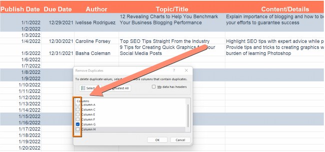
If you want to see an example, this post offers step-by-step instructions for removing duplicates.
You can also use this feature to remove an entire row based on a duplicate column value. So, say you have three rows of information and you only need to see one, you can select the whole dataset and then remove duplicates. The resulting list will have only unique data without any duplicates.
Paste Special
It’s often helpful to change the items in a row of data into a column (or vice versa). It would take a lot of time to copy and paste each individual header.
Not to mention, you may easily fall into one of the biggest, most unfortunate Excel traps — human error. Read here to check out some of the most common Microsoft Excel errors.
Instead of making one of these errors, let Excel do the work for you. Take a look at this example:
To use this function, highlight the column or row you want to transpose. Then, right-click and select «Copy.»
Next, select the cells where you want the first row or column to begin. Right-click on the cell, and then select «Paste Special.»
When the module appears, choose the option to transpose.
Paste Special is a super useful function. In the module, you can also choose between copying formulas, values, formats, or even column widths. This is especially helpful when it comes to copying the results of your pivot table into a chart.
Text to Columns
What if you want to split out information that’s in one cell into two different cells? For example, maybe you want to pull out someone’s company name through their email address. Or you want to separate someone’s full name into a first and last name for your email marketing templates.
Thanks to Microsoft Excel, both are possible. First, highlight the column where you want to split up. Next, go to the Data tab and select «Text to Columns.» A module will appear with more information. First, you need to select either «Delimited» or «Fixed Width.»
- Delimited means you want to break up the column based on characters such as commas, spaces, or tabs.
- Fixed Width means you want to select the exact location in all the columns where you want the split to occur.
Select «Delimited» to separate the full name into first name and last name.
Then, it’s time to choose the delimiters. This could be a tab, semicolon, comma, space, or something else. (For example, «something else» could be the «@» sign used in an email address.) Let’s choose the space for this example. Excel will then show you a preview of what your new columns will look like.
When you’re happy with the preview, press «Next.» This page will allow you to select Advanced Formats if you choose to. When you’re done, click «Finish.»
Format Painter
Excel has a lot of features to make crunching numbers and analyzing your data quick and easy. But if you ever spent some time formatting a spreadsheet, you know it can get a bit tedious.
Don’t waste time repeating the same formatting commands over and over again. Use the format painter to copy formatting from one area of the worksheet to another.
To do this, choose the cell you’d like to replicate. Then, select the format painter option (paintbrush icon) from the top toolbar. When you release the mouse, your cell should show the new format.
Keyboard Shortcuts
Creating reports in Excel is time-consuming enough. How can we spend less time navigating, formatting, and selecting items in our spreadsheet? Glad you asked. There are a ton of Excel shortcuts out there, including some of our favorites listed below.
Create a New Workbook
PC: Ctrl-N | Mac: Command-N
Select Entire Row
PC: Shift-Space | Mac: Shift-Space
Select Entire Column
PC: Ctrl-Space | Mac: Control-Space
Select Rest of Column
PC: Ctrl-Shift-Down/Up | Mac: Command-Shift-Down/Up
Select Rest of Row
PC: Ctrl-Shift-Right/Left | Mac: Command-Shift-Right/Left
Add Hyperlink
PC: Ctrl-K | Mac: Command-K
Open Format Cells Window
PC: Ctrl-1 | Mac: Command-1
Autosum Selected Cells
PC: Alt-= | Mac: Command-Shift-T
Excel Formulas
At this point, you’re getting used to Excel’s interface and flying through quick commands on your spreadsheets.
Now, let’s dig into the core use case for the software: Excel formulas. Excel can help you do simple arithmetic like adding, subtracting, multiplying, or dividing any data.
- To add, use the + sign.
- To subtract, use the — sign.
- To multiply, use the * sign.
- To divide, use the / sign.
- To use exponents, use the ^ sign.
Remember, all formulas in Excel must begin with an equal sign (=). Use parentheses to make sure certain calculations happen first. For example, consider how =10+10*10 is different from =(10+10)*10.
Besides manually typing in simple calculations, you can also refer to Excel’s built-in formulas. Some of the most common include:
- Average: =AVERAGE(cell range)
- Sum: =SUM(cell range)
- Count: =COUNT(cell range)
Also note that series’ of specific cells are separated by a comma (,), while cell ranges are notated with a colon (:). For example, you could use any of these formulas:
- =SUM(4,4)
- =SUM(A4,B4)
- =SUM(A4:B4)
Conditional Formatting
Conditional formatting lets you change a cell’s color based on the information within the cell. For example, say you want to flag a category in your spreadsheet.
To get started, highlight the group of cells you want to use conditional formatting on. Then, choose «Conditional Formatting» from the Home menu. Next, select a logic option from the dropdown. A window will pop up that prompts you to provide more information about your formatting rule. Select «OK» when you’re done, and you should see your results automatically appear.
Note: You can also create your own logic if you want something beyond the dropdown choices.
Dollar Signs
Have you ever seen a dollar sign in an Excel formula? When this symbol is in a formula, it isn’t representing an American dollar. Instead, it makes sure that the exact column and row stay the same even if you copy the same formula in adjacent rows.
You see, a cell reference — when you refer to cell A5 from cell C5, for example — is relative by default.
This means you’re actually referring to a cell that’s five columns to the left (C minus A) and in the same row (5). This is called a relative formula.
When you copy a relative formula from one cell to another, it’ll adjust the values in the formula based on where it’s moved. But sometimes, you want those values to stay the same no matter whether they’re moved around or not. You can do that by making the formula in the cell into what’s called an absolute formula.
To change the relative formula (=A5+C5) into an absolute formula, precede the row and column values with dollar signs, like this: (=$A$5+$C$5).
Combine Cells Using «&»
Databases tend to split out data to make it as exact as possible. For example, instead of having data that shows a person’s full name, a database might have the data as a first name and then a last name in separate columns.
In Excel, you can combine cells with different data into one cell by using the «&» sign in your function. The example below uses this formula: =A2&» «&B2.
Let’s go through the formula together using an example. So, let’s combine first names and last names into full names in a single column.
To do this, put your cursor in the blank cell where you want the full name to appear. Next, highlight one cell that contains a first name, type in an «&» sign, and then highlight a cell with the corresponding last name.
But you’re not finished. If all you type in is =A2&B2, then there will not be a space between the person’s first name and last name. To add that necessary space, use the function =A2&» «&B2. The quotation marks around the space tell Excel to put a space between the first and last name.
To make this true for multiple rows, drag the corner of that first cell downward as shown in the example.
Pivot Tables
Pivot tables reorganize data in a spreadsheet. A pivot table won’t change the data that you have, but it can sum up values and compare information in a way that’s easy to understand.
For example, let’s look at how many people are in each house at Hogwarts.
To create the Pivot Table, go to Insert > Pivot Table. Excel will automatically populate your pivot table, but you can always change the order of the data. Then, you have four options to choose from.
Report Filter
This allows you to only look at certain rows in your dataset.
For example, to create a filter by house, choose only students in Gryffindor.
Column and Row Labels
These could be any headers or rows in the dataset.
Note: Both Row and Column labels can contain data from your columns. For example, you can drag First Name to either the Row or Column label depending on how you want to see the data.
Value
This section allows you to convert data into a number. Instead of just pulling in any numeric value, you can sum, count, average, max, min, count numbers, or do a few other manipulations with your data. By default, when you drag a field to Value, it always does a count.
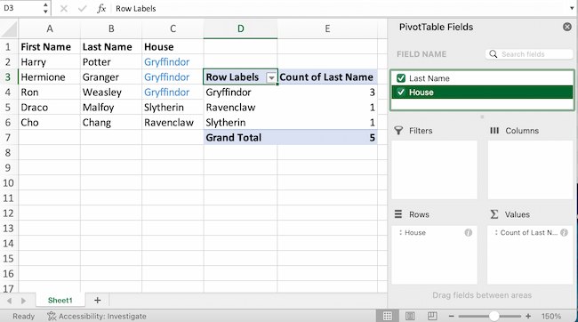
The example above counts the number of students in each house. To recreate this pivot table, go to the pivot table and drag the House column to both the row Labels and the values. This will sum up the number of students associated with each house.
IF Functions
At its most basic level, Excel’s IF function lets you see if a condition you set is true or false for a given value.
If the condition is true, you get one result. If the condition is false, you get another result.
This popular tool is useful for comparisons and finding errors. But if you’re new to Excel you may need a little more information to get the most out of this feature.
Let’s take a look at this function’s syntax:
- =IF(logical_test, value_if_true, [value_if_false])
- With values, this could be: =IF(A2>B2, «Over Budget», «OK»)
In this example, you want to find where you’re overspending. With this IF function, if your spending (what’s in A2) is greater than your budget (what’s in B2), that overspending will be easy to see. Then you can then filter the data so that you see only the line items where you’re going over budget.
The real power of the IF function comes when you string or «nest» multiple IF statements together. This allows you to set multiple conditions, get more specific results, and organize your data into more manageable chunks.
For example, ranges are one way to segment your data for better analysis. For example, you can categorize data into values that are less than 10, 11 to 50, or 51 to 100.
- =IF(B3<11,»10 or less»,IF(B3<51,»11 to 50″,IF(B3<100,»51 to 100″)))
Let’s talk about a few more IF functions.
COUNTIF Function
The power of IF functions goes beyond simple true and false statements. With the COUNTIF function, Excel can count the number of times a word or number appears in any range of cells.
For example, let’s say you want to count the number of times the word «Gryffindor» appears in this data set.
Take a look at the syntax.
- The formula: =COUNTIF(range, criteria)
- The formula with variables from the example below: =COUNTIF(D:D,»Gryffindor»)
In this formula, there are several variables:
Range
The range that you want the formula to cover.
In this one-column example, «D:D» shows that the first and last columns are both D. If you want to look at columns C and D, use «C:D.»
Criteria
Whatever number or piece of text you want Excel to count.
Only use quotation marks if you want the result to be text instead of a number. In this example, «Gryffindor» is the only criteria.
To use this function, type the COUNTIF formula in any cell and press «Enter.» Using the example above, this action will show how many times the word «Gryffindor» appears in the dataset.
SUMIF Function
Ready to make the IF function a bit more complex? Let’s say you want to analyze the number of leads your blog has generated from one author, not the entire team.
With the SUMIFS function, you can add up cells that meet certain criteria. You can add as many different criteria to the formula as you like.
Here’s your formula:
- =SUMIFS(sum_range, criteria_range1, criteria1, [criteria_range2, criteria 2],etc.)
That’s a lot of criteria. Let’s take a look at each part:
Sum_range
The range of cells you’re going to add up.
Criteria_range1
The range that is being searched for your first value.
Criteria1
This is the specific value that determines which cells in Criteria_range1 to add together.
Note: Remember to use quotation marks if you’re searching for text.
In the example below, the SUMIF formula counts the total number of house points from Gryffindor.

If AND/OR
The OR and AND functions round out your IF function choices. These functions check multiple arguments. It returns either TRUE or FALSE depending on if at least one of the arguments is true (this is the OR function), or if all of them are true (this is the AND function).
Lost in a sea of «and’s» and «or’s»? Don’t check out yet. In practice, OR and AND functions will never be used on their own. They need to be nested inside of another IF function. Recall the syntax of a basic IF function:
- =IF(logical_test, value_if_true, [value_if_false])
- Now, let’s fit an OR function inside of the logical_test: =IF(OR(logical1, logical2), value_if_true, [value_if_false])
To put it plainly, this combined formula allows you to return a value if both conditions are true, as opposed to just one. With AND/OR functions, your formulas can be as simple or complex as you want them to be, as long as you understand the basics of the IF function.
VLOOKUP
Have you ever had two sets of data on two different spreadsheets that you want to combine into a single spreadsheet?
For example, say you have a list of names and email addresses in one spreadsheet and a list of email addresses and company names in a different spreadsheet. But you want the names, email addresses, and company names of those people to appear in one spreadsheet.
VLOOKUP is a great go-to formula for this.
Before you use the formula, be sure that you have at least one column that appears identically in both places.
Note: Scour your data sets to make sure the column of data you’re using to combine spreadsheets is exactly the same. This includes removing any extra spaces.
In the example below, Sheet One and Sheet Two are both lists with different information about the same people. The common thread between the two is their email addresses. Let’s combine both datasets so that all the house information from Sheet Two translates over to Sheet One.
Type in the formula: =VLOOKUP(C2,Sheet2!A:B,2,FALSE). This will bring all the house data into Sheet One.
Now that you’ve seen how VLOOKUP works, let’s review the formula.
- The formula: =VLOOKUP(lookup value, table array, column number, [range lookup])
- The formula with variables from the example: =VLOOKUP(C2,Sheet2!A:B,2,FALSE)
In this formula, there are several variables.
Lookup Value
A value that LOOKUP searches for in an array. So, your lookup value is the identical value you have in both spreadsheets.
In the example, the lookup value is the first email address on the list, or cell 2 (C2).
Table Array
Table arrays hold column-oriented or tabular data, like the columns on Sheet Two you’re going to pull your data from.
This table array includes the column of data identical to your lookup value in Sheet One and the column of data you’re trying to copy to Sheet Two.
In the example, «A» means Column A in Sheet Two. The «B» means Column B.
So, the table array is «Sheet2!A:B.»
Column Number
Excel refers to columns as letters and rows as numbers. So, the column number is the selected column for the new data you want to copy.
In the example, this would be the «House» column. «House» is column 2 in the table array.
Note: Your range can be more than two columns. For example, if there are three columns on Sheet Two — Email, Age, and House — and you also want to bring House onto Sheet One, you can still use a VLOOKUP. You just need to change the «2» to a «3» so it pulls back the value in the third column. The formula for this would be: =VLOOKUP(C2:Sheet2!A:C,3,false).]
Range Lookup
This term means that you’re looking for a value within a range of values. You can also use the term «FALSE» to pull only exact value matches.
Note: VLOOKUP will only pull back values to the right of the column containing your identical data on the second sheet. This is why some people prefer to use the INDEX and MATCH functions instead.
INDEX MATCH
Like VLOOKUP, the INDEX and MATCH functions pull data from another dataset into one central location. Here are the main differences:
VLOOKUP is a much simpler formula.
If you’re working with large datasets that need thousands of lookups, the INDEX MATCH function will decrease load time in Excel.
INDEX MATCH formulas work right-to-left.
VLOOKUP formulas only work as a left-to-right lookup. So, if you need to do a lookup that has a column to the right of the results column, you’d have to rearrange those columns to do a VLOOKUP. This can be tedious with large datasets and lead to errors.
Let’s look at an example. Let’s say Sheet One contains a list of names and their Hogwarts email addresses. Sheet Two contains a list of email addresses and each student’s Patronus.
The information that lives in both sheets is the email addresses column. But, the column numbers for email addresses are different on the two sheets. So, you’d use the INDEX MATCH formula instead of VLOOKUP to avoid column-switching errors.
The INDEX MATCH formula is the MATCH formula nested inside the INDEX formula.
- The formula: =INDEX(table array, MATCH formula)
- This becomes: =INDEX(table array, MATCH (lookup_value, lookup_array))
- The formula with variables from the example: =INDEX(Sheet2!A:A,(MATCH(Sheet1!C:C,Sheet2!C:C,0)))
Here are the variables:
Table Array
The range of columns on Sheet Two that contain the new data you want to bring over to Sheet One.
In the example, «A» means Column A, and has the «Patronus» information for each person.
Lookup Value
This Sheet One column has identical values in both spreadsheets.
In the example, this is the «email» column on Sheet One, which is Column C. So, Sheet1!C:C.
Lookup Array
Again, an array is a group of values in rows and columns that you want to search.
In this example, the lookup array is the column in Sheet Two that contains identical values in both spreadsheets. So, the «email» column on Sheet Two, Sheet2!C:C.
Once you have your variables set, type in the INDEX MATCH formula. Add it where you want the combined information to populate.
Data Visualization
Now that you’ve learned formulas and functions, let’s make your analysis visual. With a beautiful graph, your audience will be able to process and remember your data more easily.
Create a Basic Graph
First, decide what type of graph to use. Bar charts and pie charts help you compare categories. Pie charts compare part of a whole and are often best when one of the categories is way larger than the others. Bar charts highlight incremental differences between categories. Finally, line charts can help display trends over time.
This post can help you find the best chart or graph for your presentation.
Next, highlight the data you want to turn into a chart. Then choose «Charts» in the top navigation. You can also use Insert > Chart if you have an older version of Excel. Then you can adjust and resize your chart until it makes the statement you’re hoping for.
Microsoft Excel Can Help Your Business Grow
Excel is a useful tool for any small business. Whether you’re focused on marketing, HR, sales, or service, these Microsoft Excel tips can boost your performance.
Whether you want to improve efficiency or productivity, Excel can help. You can find new trends and organize your data into usable insights. It can make your data analysis easier to understand and your daily tasks easier.
All it takes is a little know-how and some time with the software. So start learning, and get ready to grow.
Editor’s note: This post was originally published in April 2018 and has been updated for comprehensiveness.

Microsoft Excel — программа, позволяющая работать с электронными таблицами. Можно собирать, преобразовывать и анализировать данные, проводить визуализацию информации, автоматизировать вычисления и выполнять еще ряд полезных и необходимых в работе задач.
Изучение возможностей Excel может быть полезно в рамках практически любой профессии и сферы деятельности, от работников продаж до бухгалтеров и экономистов.
Возможности Microsoft Excel
Работа с формулами и числовыми данными
Excel может выполнять практически всё: от простых операций вроде сложения, вычитания, умножения и деления до составления бюджетов крупных компаний.
Работа с текстом
Несмотря на то что некоторые возможности Word в Excel неприменимы, программа очень часто является базовой для составления отчетов.
Организация баз данных
Excel — табличный редактор, поэтому систематизация больших архивов не является для него проблемой. Кроме того, благодаря перекрестным ссылкам можно связать между собой различные листы и книги.
Построение графиков и диаграмм
Для создания отчетов очень часто требуется их визуальное представление. В современных версиях Excel можно создать диаграммы и графики любого типа, настроив их по своему усмотрению.
Создание рисунков
С помощью настройки графических объектов, встроенных в программу, можно создавать двухмерные и трехмерные рисунки.
Автоматизация стандартных задач
Excel обладает функцией записи макросов, которые облегчают работу с однотипными действиями. Под любой макрос можно создать отдельную кнопку на рабочей панели или установить сочетание горячих клавиш.
Импорт и экспорт данных
Для создания масштабных отчетов можно загружать данные различных типов со сторонних ресурсов.
Собственный язык программирования
Язык программирования Visual Basic позволяет сделать работу в программе максимально удобной. Большое количество встроенных функций помогают сделать таблицы интерактивными, что упрощает восприятие.
Интерфейс Excel
В настоящий момент самой современной, 16-й версией программы является Excel 2019. Обновления, появляющиеся с каждой новой версией, касаются прежде всего новых формул и функций. Начальный рабочий стол с версии 2007 года претерпел мало изменений.
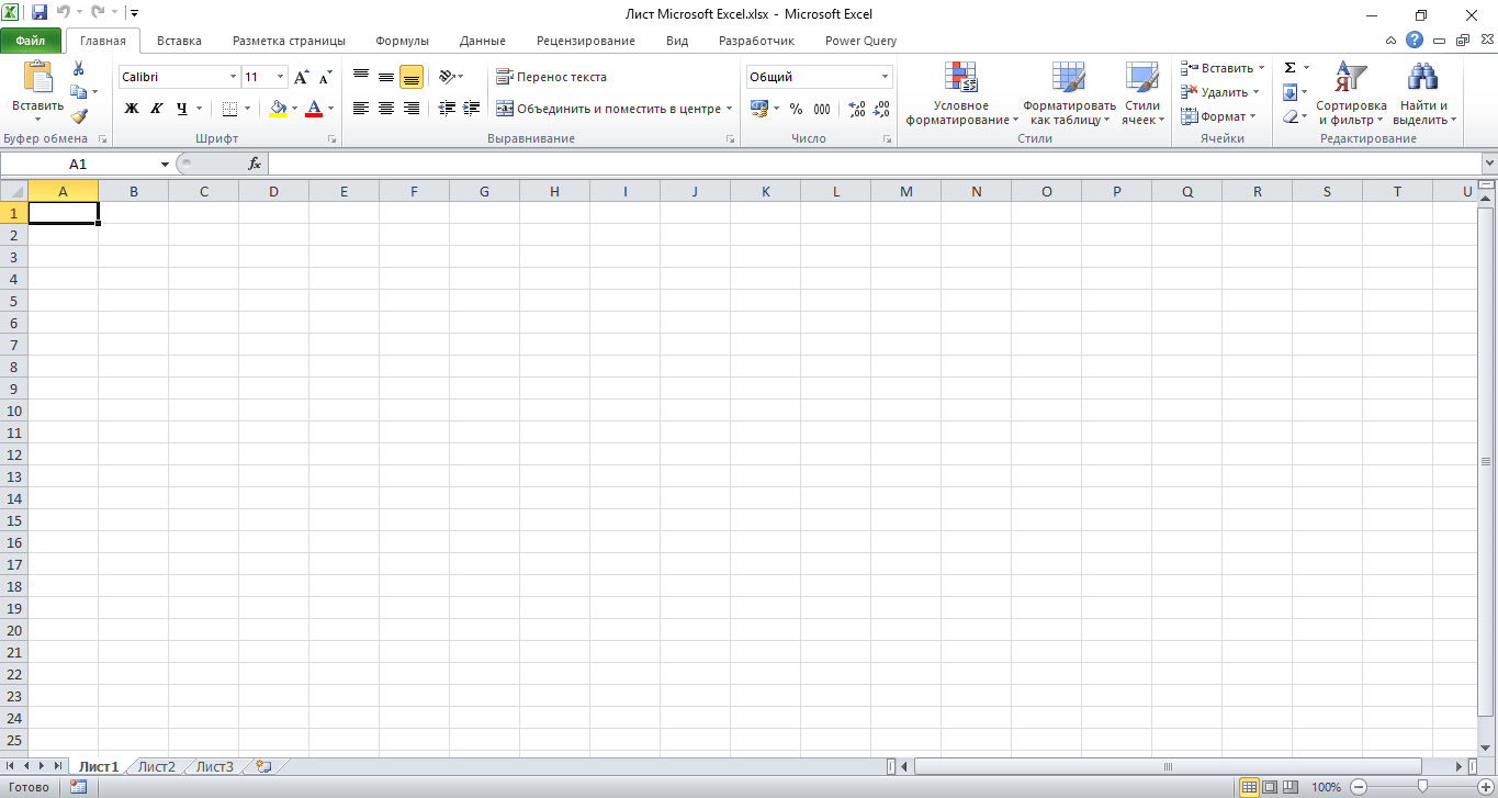
По умолчанию в каждой книге присутствует один лист (в ранних версиях — три листа). Количество листов, которые можно создавать в одной книге, ограничено только возможностями оперативной памяти компьютера. Поле Excel представляет собой таблицу из ячеек. Каждая ячейка имеет свой уникальный адрес, образованный пересечением строк и столбцов. Всего в Excel 1 048 576 строк и 16 384 столбца, что дает 2 147 483 648 ячеек. Над полем с ячейками находится строка функций, в которой отображаются данные, внесенные в ячейки или формулы. Также в программе есть несколько вкладок, которые мы разберем подробнее.
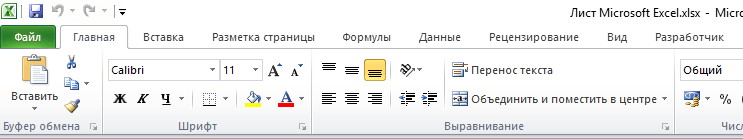
«Файл». С помощью этой вкладки можно отправить документы на печать, установить параметры работы в программе и сделать другие базовые настройки.
«Главная». Здесь располагается основной набор функций: возможность смены параметров шрифта, сортировка данных, простейшие формулы и правила условного форматирования.
«Вставка». Вкладка предназначена для добавления графических элементов на лист. Пользователь может как добавить обычные рисунки и фотографии, так и создать 2D- и 3D-объекты через конструктор. Кроме того, один из самых важных разделов программы — графики и диаграммы — также находится здесь.
«Разметка страницы». Здесь пользователь может менять формат итогового файла, работать с темой и подложкой.
«Формулы». Все формулы и функции, с которыми пользователь может работать в программе, собраны в этой вкладке и рассортированы по соответствующим разделам.
«Данные». Вкладка помогает с фильтрацией текстовых и числовых значений в таблицах, позволяет импортировать данные из других источников.
«Рецензирование». Здесь можно оставлять примечания к ячейкам, а также устанавливать защиту листа и всей книги.
«Вид». На этой вкладке можно добавлять или убирать сетку таблицы, масштабировать значения, закреплять группы данных в таблицах.
«Разработчик». Дополнительная вкладка, которая не включена по умолчанию. Позволяет работать с Visual Basic, создавать новые макросы и запускать уже имеющиеся.
Форматы файлов
Для Excel существует несколько форматов готовых файлов, которые определяют возможности книги:
- .xlsx — стандартная рабочая книга. Пришла на смену бинарному формату .xls с версии 2007 года;
- .xlsm — рабочая книга, позволяющая работать с макросами;
- .xlsb — рабочая книга, использующая бинарный формат, но одновременно и поддерживающая макросы. Обычно используется при работе с большими таблицами;
- .xltm — шаблон-основа для рабочих книг. Имеется поддержка макросов;
- .xlam — надстройка, созданная для добавления дополнительного функционала.
Нужно учитывать, что некоторые формулы и функции из новых версий могут не работать в старых.
Стандартные операции с ячейками
Активной считается ячейка, которая имеет черную рамку выделения с квадратом в правом нижнем углу. Чтобы вносить данные в ячейку, не обязательно делать по ней дополнительные клики мышью. Вносить данные можно как непосредственно в ячейку, так и через строку формул. При перемещении курсора с помощью клавиш-стрелок активной становится соседняя ячейка, текст в предыдущей сохраняется. Чтобы изменить уже имеющийся текст, необходимо дважды кликнуть по ячейке или внести правки через строку формул.
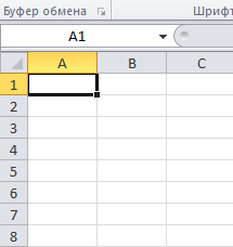
При двойном клике по черному квадрату в правом нижнем углу текстовые данные протянутся до нижнего края созданной таблицы. Если выделить диапазон с последовательными значениями (числа, даты, дни недели), они автоматически пересчитаются в сторону увеличения, заполнив столбец до нижнего края таблицы. Те же операции можно проделать и вручную, протянув за квадрат в нижнем правом углу. В этом случае пользователь самостоятельно определяет границы заполнения.
Чтобы выделить несколько ячеек одновременно, нужно зажать клавишу Ctrl и выбрать нужные ячейки или диапазоны ячеек. Ту же самую операцию можно проделать со строками и столбцами, выделяя необходимое их количество.
Excel автоматически суммирует значения в ячейках, показывая результат в правом нижнем углу листа. Также пользователю предлагаются средние значения данных и общее количество заполненных ячеек.
Ширину столбцов и высоту строк можно менять как вручную, передвигая край столбца/строки, так и нажав правую клавишу мыши и выбрав меню «Ширина столбца (высота строки)». По умолчанию значение ширины указывает на количество символов текущего размера шрифта, которые могут разместиться в ячейке, а значение высоты — на максимально возможный размер шрифта для этой строки.
Ячейки можно объединять с помощью соответствующего меню на вкладке «Главная». Всего существует три варианта объединения:
- объединить и поместить в центре;
- объединить по строкам;
- объединить ячейки.
Следует помнить, что при объединении может нарушаться сортировка данных в таблицах, а также могут некорректно считаться формулы.
Работа с формулами Excel
Главная функция программы — возможность подсчета значений с помощью встроенных формул и функций. Среди них есть простые, позволяющие подсчитать сумму в диапазоне, среднее значение в диапазоне, количество заполненных ячеек и т.д. Есть и более сложные, способные вычислять количество дней между разными датами (в т.ч. рабочих), максимальные и минимальные значения в диапазоне. Работа с функциями и формулами также напрямую зависит от формата ячеек. По умолчанию для всех ячеек установлен общий формат, позволяющий работать как с числовыми, так и с текстовыми данными. Но для более сложной работы он может быть заменен на числовой, процентный, дату, денежный, финансовый, дробный и т.д.
Формула вводится либо через строку функций над таблицей, либо в самой ячейке при двойном клике. В начале функции обязательно должен стоять знак «=». После этого при вводе названия функции появляется помощник, который предлагает выбрать функции из списка. Разберем это на примере формулы средней сложности «СЧЕТЕСЛИ».
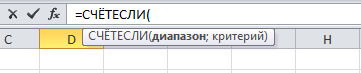
В скобках после функции будут прописаны условия, по которым формула будет проводить вычислениях. Подсказка указывает на то, что потребуется задать диапазон вычислений и критерий, по которому они будут производиться.
Например, нам необходимо подсчитать количество букв «А» в указанном диапазоне:
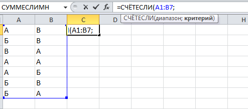
Выделяем диапазон, отмечаем первое условие с помощью знака «;»
Далее выделяем критерий. Его можно прописать вручную, заключив в кавычки; можно выделить ячейку, в которой этот критерий прописан.
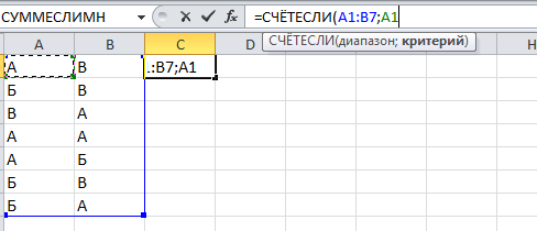
Закрываем скобку, потому что все условия указаны, и нажимаем Enter.
В ячейке C1 получаем ответ: в шести ячейках нашей таблицы написана буква «А».
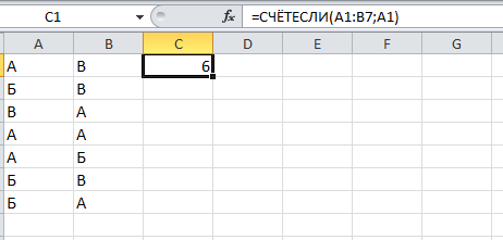
В случае ошибки в формулах в ячейке будет прописано «#ДЕЛ/0!». В этом случае необходимо перепроверить формулу на предмет неточностей и на корректность.
Excel может проводить вычисления не только на активном листе. Для этого при вводе формулы через строку функций нужно перейти на нужный лист и указать ячейку, с которой нужно провести расчет. При протягивании формул автоматически подтянутся и адреса всех ячеек. Чтобы этого не произошло и формулы были подсчитаны корректно, можно закрепить нужную ячейку, выделив ее адрес и нажав клавишу F4. Формат адреса будет выглядеть так: $A$1.