
Excel for Microsoft 365 Excel for Microsoft 365 for Mac Excel for the web More…Less

Data on hundreds of subjects like cities, foods, animals, constellations, and more, all right in Excel. With linked data types, you gain access to a trusted database brimming with facts and data, templates to get things done, and more. These data types make it possible to accomplish goals for real life with the power and flexibility of Excel.
Data types transform the way you work with data
Real data for real life
Explore the universe or start a film club? With tons of data types with facts on a variety of subjects, the possibilities are almost limitless.
Convenience and efficiency
No more pasting from browsers or skimming search results. Data types make it easy to compile and bring facts from trusted sources right into Excel.
Use dynamic and flexible datasets
Easily explore data in Excel with interactive cards that hold a variety of data in a single cell. Insert, refresh, and work with data the way you want.
Start quickly with smart templates
Our data type templates help get things done fast, such as comparing colleges, tracking investments, planning a movie nights, and more.
Want more?
Linked data types FAQ and tips
Convert text to a linked data type in Excel
Stocks and geography data types
Discover more from Wolfram
Give feedback about data types
Need more help?
Want more options?
Explore subscription benefits, browse training courses, learn how to secure your device, and more.
Communities help you ask and answer questions, give feedback, and hear from experts with rich knowledge.
Linking Data allows you to input data from one worksheet into another worksheet in such a way that it will change if the original data is changed.
This can be used to prevent your spreadsheet from needing to hold multiple copies of the same data.
For example, maintaining one master price list and linking any other spreadsheet that needs that same information to it.
This helps maintain data accuracy as only one spreadsheet needs to be updated for price changes.
It is an excellent way to make it very simple to create a summary of up to date data.
This becomes especially important when multiple people are working on the same spreadsheet.
If the data inputs are not logically presented and organised, it is impossible for someone else to update the spreadsheet accurately.
There are two methods to link data with.
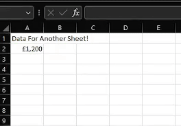
Before we start, here is what a sheet of the source data in excel looks like:
If you want your data to be better delineated, you can follow our guide on creating borders here.
Method 1 – Cell Formula Writing + Clicking
- First, click the cell in the worksheet you want the data to appear in
- Type in the formula bar “=”
- Click on the information in the source worksheet you want to carry across
- Press enter
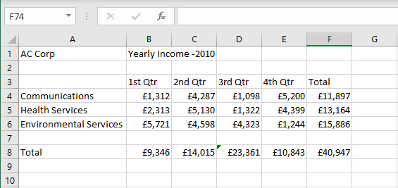
The formula bar will show where the information has been linked to, the sheet name, an exclamation mark and the cell number:
Note you can link to named ranges as well as cells.
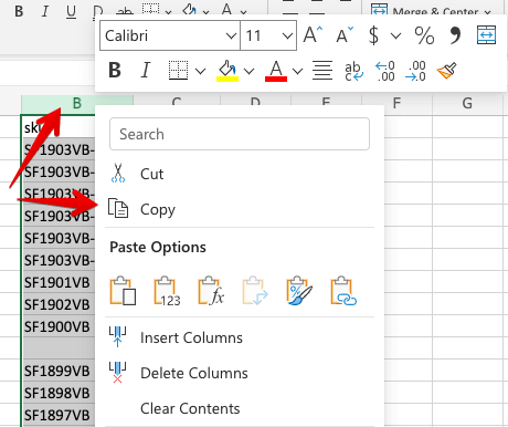
Method 2 – Copy And Paste
- Start on the source worksheet and copy the information you want to link
- Right click on the cell in the destination sheet and go to ‘Paste special’
- Click on the ‘Data link’ icon. Interestingly, if you are used to opening up the paste special box, the data link option doesn’t appear in it.
If you use this method, the cell is entered as an absolute cell reference. You can learn all about all types of cell references with this comprehensive guide.
Linking to Multiple Cells
You can also create a link to multiple sheets and cells to a single cell with a function.
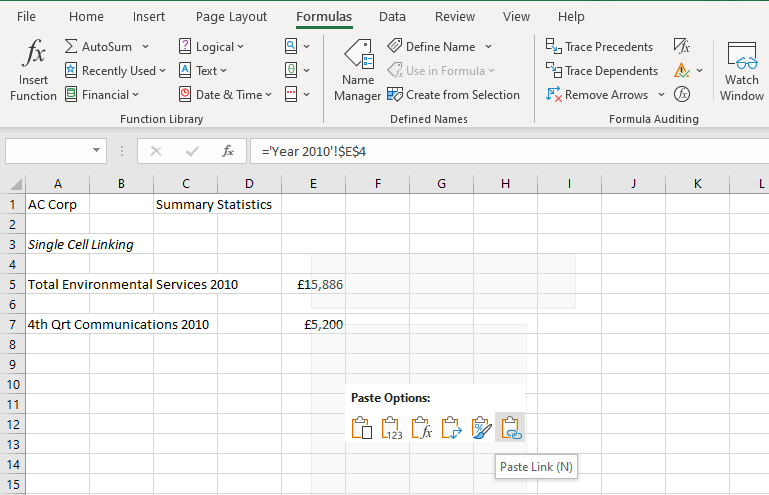
In the example below, the total spend on communications for three years has been shown on the summary sheet:
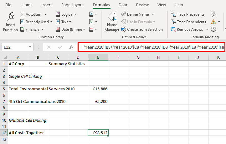
To do this, you will use method 1 above but after clicking on the first total in 2010, press ‘+’ then click the next piece of data and so on.
Microsoft Excel offers lots of different ways to validate and track your data in larger, more complex spreadsheets.
For more details on linking data this is covered in our Excel courses.
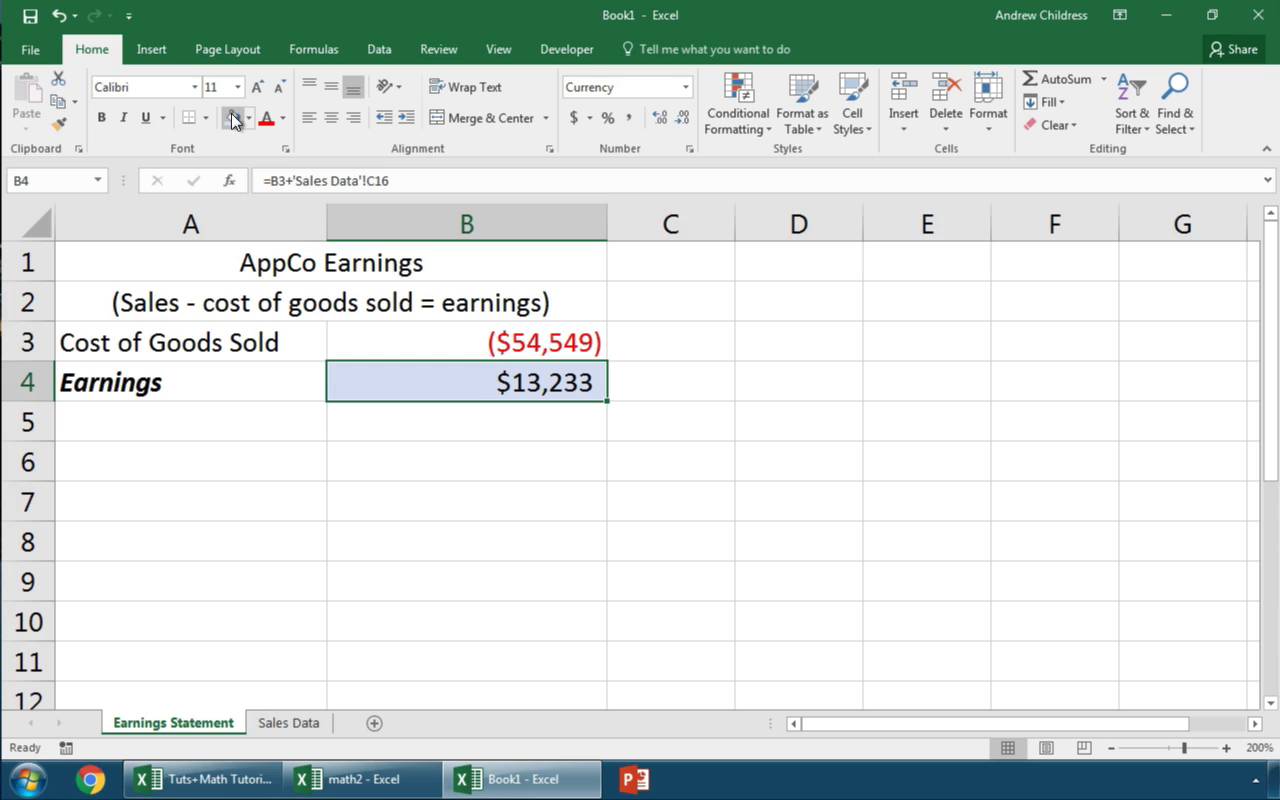
As you use and build more Excel workbooks, you’ll need to link them up. Maybe you want to write formulas that use data between different sheets in a workbook. You can even write formulas that use data from multiple different workbooks.
If I want to keep my files clean and tidy, I’ve found it’s best to separate large sheets of data from the formulas that summarize them. I often use a single workbook or sheet to summarize things.
In this tutorial, you’ll learn how to link data in Excel. First, we’ll learn how to link up data in the same workbook on different sheets. Then, we’ll move on to linking up multiple Excel workbooks to import and sync data between files.
How to Quickly Link Data in Excel Workbooks (Watch & Learn)
I’ll walk you through two examples linking up your spreadsheets. You’ll see how to pull data from another workbook in Excel and keep two workbooks connected. We’ll also walk through a basic example to write formulas between sheets in the same workbook.
Let’s walk through an illustrated guide to linking up your data between sheets and workbooks in Excel.
Basics: How to Link Between Sheets in Excel
Let’s start off by learning how to write formulas using data from another sheet. You probably already know that Excel workbooks can contain multiple worksheets. Each worksheet is a tab of its own, and you can switch tabs by clicking on them at the bottom of Excel.
Complex workbooks can easily grow to many sheets. In time, you’ll certainly need to write formulas to work with data on different tabs.
Maybe you use a single sheet in your workbook for all of your formulas to summarize your data, and separate sheets to hold the original data.

Let’s learn how to write a multi-sheet formula to work with data from multiple sheets in the same workbook.
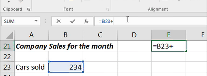
1. Start a New Formula in Excel
Most formulas in Excel start off with the equals (=) sign. Double click or start typing in a cell and begin writing the formula that you want to link up. For my example, I’ll write a sum formula to add up several cells.
I’ll open up the = sign, and then click on the first cell on my current sheet to make it the first part of the formula. Then, I’ll type a + sign to add my second cell to this formula.
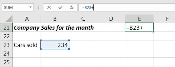

Now, make sure that you don’t close out your formula and press enter yet! You’ll want to leave the formula open before you switch sheets.
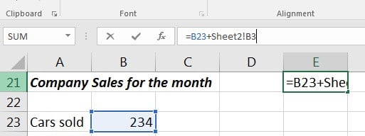
2. Switch Sheets in Excel
While you still have the formula open, click on a different sheet tab at the bottom of Excel. It’s very important that you don’t close out the formula before you click on the next cell to include as part of the formula.

After you switch sheets, click on the next cell that you want to include in the formula. As you can see in the screenshot below, Excel automatically writes the part of the formula that references a cell on another sheet for you.
Notice in the screenshot below that to reference a cell on another sheet, Excel adds «Sheet2!B3», which simply references cell B3 on a sheet named Sheet2. You could write this manually, but clicking on the cells makes Excel write it for you automatically.

3. Finish the Excel Formula
At this point, you can press enter to close out and complete your multi-sheet formula. When you do so, Excel will jump back to where you started the formula and show you the results.
You could also keep writing the formula, including cells from more sheets and other cells on the same sheet. Keep combining those references throughout the workbook for all the data you need.
Level Up: How to Link Multiple Excel Workbooks
Let’s learn how to pull data from another workbook. With this skill, you can write formulas that pull together data from entirely separate Excel workbooks.
For this section of the tutorial, you can use two workbooks that you can download for free as a part of this tutorial. Open them both up in Excel, and follow the directions below.
1. Open Both Workbooks
Let’s start off by writing a formula that includes data from two different workbooks.
The easiest way to use this feature is to open up two Excel workbooks at the same time and put them side by side. I use the Windows Snap feature to split them to each take up half the screen. You need to keep both workbooks in view to write formulas between them.
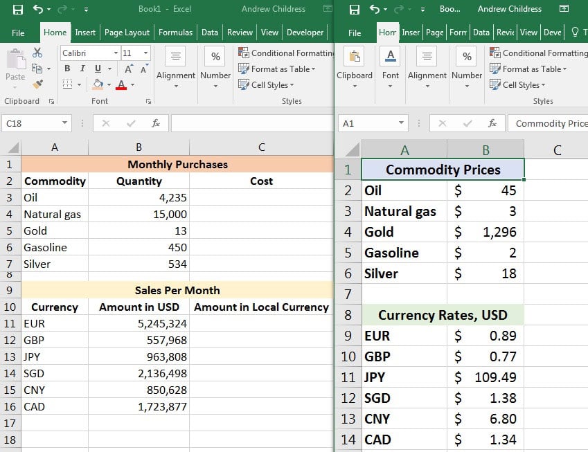
In the screenshot below, I’ve opened two workbooks that I’ll write formulas for side-by-side. For my example, I’m running a business that buys a variety of products, and sells them in a variety of countries. So, I’ll use separate workbooks to track my purchases/sales and cost data.

2. Start Writing Your Formula in Excel
The price of what I buy can change, and so can the rate that I receive payments in. I need to keep a lookup list of rates and multiply it times my purchases. This is the perfect time to link two workbooks together and write formulas between them.
Let’s take the number of barrels of oil I buy each month times the price per barrel. In the first Cost cell (cell C3), I’ll start writing a formula by typing the equals sign (=), and then clicking on cell B3 to grab the quantity. Now, I’ll add an * to prepare to multiply the quantity by the rate.
So far, your formula should be:
=B3*


Don’t close out your formula yet. Make sure to leave it open before moving onto the next step; we still need to point Excel to the price data to multiply the quantity by.
3. Switch Excel Workbooks
It’s time to switch workbooks, and this is why it’s important to keep both of your datasets in view while working between workbooks.
With your formula still open, click over to the other workbook. Then, click on a cell in your second workbook to link up the two Excel files.


Excel automatically wrote the reference to a separate workbook as part of the cell formula:
=B3*[Prices.xlsx]Sheet1!$B$2
Once you press Enter, Excel will calculate the final cost by multiplying the quantity in the first workbook times the price in the second workbook.
Now, keep working on your Excel skills by multiplying each of the quantities or values times the reference amounts in the «Prices» workbook.
In short, the key is to get your workbooks open side by side, and simply switch workbooks to write formulas referencing other files.
There’s nothing stopping you from linking up more than two workbooks. You could open many workbooks to link up and write formulas, connecting the data between many sheets to keep cells up to date.
How to Refresh Your Data Between Workbooks
When you’ve written formulas that reference other Excel workbooks, you’ll need to think about how you’ll update your data.
So, what happens when the data changes in the workbook that you’re linking to? Will your workbook automatically update, or will you need to refresh your files to pull over the last data and import it?
The answer is, «it depends», and specifically, it depends upon if both workbooks are still open at the same time.
Example 1: Both Excel Workbooks Still Open
Let’s check out an example using the same workbook from the prior step. Both workbooks are still open. Let’s see what happens when we change the price of oil from $45 per barrel to $75 per barrel:


In the screenshot above, you can see that when we updated the price of oil, the other workbook automatically updated.
This is important to know: if both workbooks are open at the same time, changes will update automatically and in real-time. When you change one variable, the other workbook will update or recalculate based upon the new value.
Example 2: With One Workbook Closed
What if you only open one workbook at a time? For example, each morning, we update prices of our commodities and currencies, and in the evening we review the impact of the change to our purchases and sales.
The next time you open up your workbook that references other sheets, you might get a message similar to the one below. You can click on Update to pull in the latest data from your reference workbook.
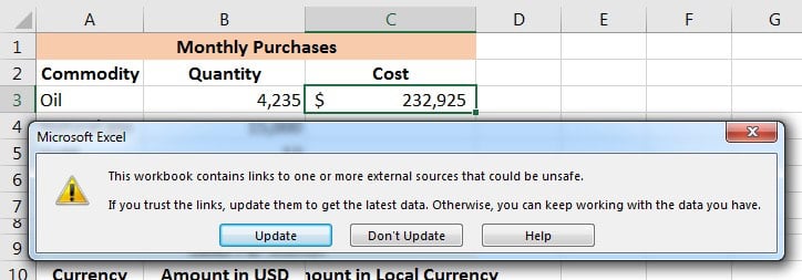


You might also see a menu where you can click Enable Content to automate updating data between Excel files.
Recap and Keep Learning More About Excel
Writing formulas between sheets and workbooks is a necessary skill when you work with Microsoft Excel. Using multiple spreadsheets inside your formulas is no problem with a bit of know-how.
Check out these additional tutorials to learn more about Excel skills and how to work with data. These tutorials are a great way to continue learning Excel.
Let me know in the comments if you have any questions about how to link up your Excel workbooks.
Did you find this post useful?

I believe that life is too short to do just one thing. In college, I studied Accounting and Finance but continue to scratch my creative itch with my work for Envato Tuts+ and other clients. By day, I enjoy my career in corporate finance, using data and analysis to make decisions.
I cover a variety of topics for Tuts+, including photo editing software like Adobe Lightroom, PowerPoint, Keynote, and more. What I enjoy most is teaching people to use software to solve everyday problems, excel in their career, and complete work efficiently. Feel free to reach out to me on my website.
Working with Excel, a day will come when you’ll need to reference data from one workbook in another one. It’s a common use case and pretty easy to pull off. Join us as we explain how to link two Excel files and discuss many possible scenarios.
How to link Excel files – what are the available options?
Just as there are many different versions of Excel, the ways to link data also differ. It’s a lot easier if you share your Excel files in OneDrive rather than locally but we’ll discuss both scenarios.
Choosing how to link data depends also on the sheer volume of what you wish to link. If we’re talking here about particular cells or a column from your workbook, the default methods will do just fine. If you’re after linking entire Excel files, using tools such as Coupler.io with its Excel integrations may prove to be more efficient. But we’ll get to that!
You can link two or more Excel files stored on your hard drive. When the data changes in a Source file, the change will be quickly reflected in the Destination file.
The drawback of this approach is that it will only work on your local machine. Even if you share both files with another user, the link will cease to exist and they’ll be forced to re-add it. What’s more, the data will be only updated if both files are open at the same time.
So if you have a choice, it’s better to add both files to your OneDrive. If they’re already in there, you may as well jump to the How to link between Cloud-based Excel files section.
To link 2 Excel files stored locally, you have two options:
- Type in a formula referencing the exact location in a Source file
- Copy the desired cells and paste them as a link
How to link between files in desktop Excel?
To reference a single cell in another local file, you’ll use the following formula:
=[SourceWorkbook.xlsx]Sheet1!$A$1
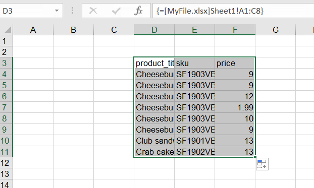
Replace SourceWorkbook.xlsx with the name of the file stored on your machine. Then, point to an exact sheet and a cell. A reference to a range of cells could like this:
=[MyFile.xlsx]Sheet1!A1:C8
Press ENTER to save the formula and pull the data. If you’re on an older version of Excel, you may need to press CTRL+SHIFT+ENTER instead.
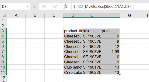
When you close the Source file, the formulas will change to include the entire path of the file – for example:
='C:[MyFile.xlsx]Sheet1'!A1:C8
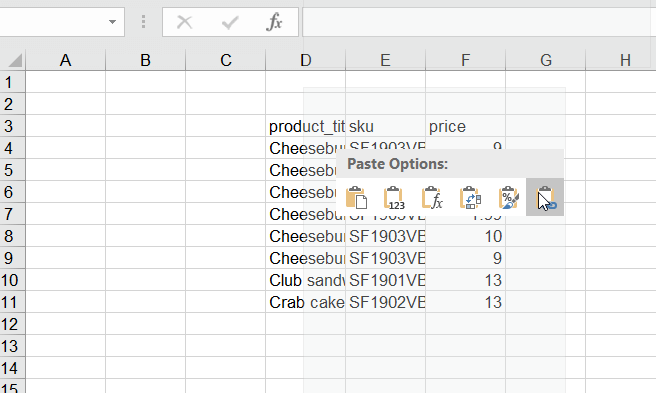
As an alternative, you can:
- Open a Source file, select the desired cells, and copy them.

- Head back to the Destination file, right-click on a desired cell or cells and choose to paste as a link.

- Here is the result:
Note that if the Source file is closed, and you reference it with a formula, no data will be pulled until you open a file.
How to link between cloud-based files in Excel?
When you wish to link Excel Online files or use those stored in OneDrive, things become easier. You can freely share files among coworkers and any interlinking won’t be affected. Links in files also refresh in near real time, giving you peace of mind that you’re working with the latest data.
The feature that enables it is called Workbook Links. We’ll explain how it works in the following chapters.
Workbook Links are suitable for individual cells or ranges of them. You may also link individual columns but the more data is involved, the slower your calculations will be. If you’re going to be linking entire worksheets or workbooks, it’s far better to focus on importing, rather than linking them. This is best done with dedicated tools.
There is more on that in the How to link a wide range of cells to Excel or another service chapter.
How to link two Excel files?
Let’s start with a most basic use case – you’re running some operations in your Excel workbook. In one of the fields, you wish to use the value(s) from another workbook and have it update automatically.
The flow is simple:
- In workbook 1 (source), highlight the data you want to link and copy it.
- In workbook 2 (destination), right-click on the first row and select the Link icon.

The latest data will be imported. A yellow bar will, however, appear now as well as every time you open a destination workbook.

To enable the data sync, select Enable Content.
For some more advanced settings, you can choose the Manage Workbook Links button to look up the list of connected workbooks and a status for each – most likely it will be Connection Blocked.
To sync, press the Enable Content button from the yellow bar.

If any errors occur, you’ll see them in the menu to the right. For each of the connected files, you can press the Refresh button to manually pull the latest data. You can also use the button above to refresh data for all your links.
Of course, the whole idea of creating links between workbooks is not to keep refreshing the data manually. Once the data has been refreshed, an option to set automatic updates will be enabled.
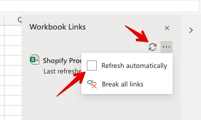
If you tick Refresh automatically, the data will start to refresh periodically.
How to link a wide range of cells to Excel or another service?
The more data you link, the more computing your Excel needs to perform to pull the data and refresh it. It’s not an issue if you have a few or a few dozens of links spread across files.
However, if you wish to regularly pull thousands of cells into your workbooks, it will significantly slow down your workbooks. It may delay the data refresh and may leave you wondering whether the data has already been refreshed or not.
To avoid that, for larger operations it’s better to use tools dedicated to importing data such as Coupler.io. With Coupler.io, you can pull the desired ranges of cells directly into another Excel workbook or worksheet. You can then refresh the data automatically at a chosen schedule.
If you wish to, you can also import the Excel data to other services, such as Google Sheets or Google BigQuery, or bring it to Excel from Airtable, Pipedrive, Hubspot, and many others.
To get started with Coupler.io, create an account, log in, and click the Add an importer button.
From the list of source applications, choose Excel.

Next, click the Connect button. Log in with your Microsoft account and allow for Coupler.io to connect.
Once connected, you’ll need to choose the workbook from your OneDrive that we’ll be importing from. Also select the worksheet in this file.
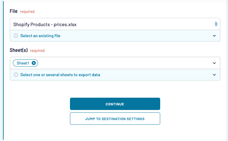
Although it’s optional, most often you’ll want to specify the range of cells to import. If you don’t, all data from a given sheet will be fetched.
You may use the standard Excel formatting and pull, for example, cells C1:D8. You may also pull an entire column by typing, for example, C1:C.

Jumping to the Destination settings, choose where to import the data to. We’ll go with Excel as we just want to move the data from one workbook to another but there are other options available too.
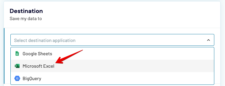
If you’re importing from Excel to Excel, there’s no need to connect your account again, unless you’re importing to someone else’s account. Select it, and specify the exact destination.
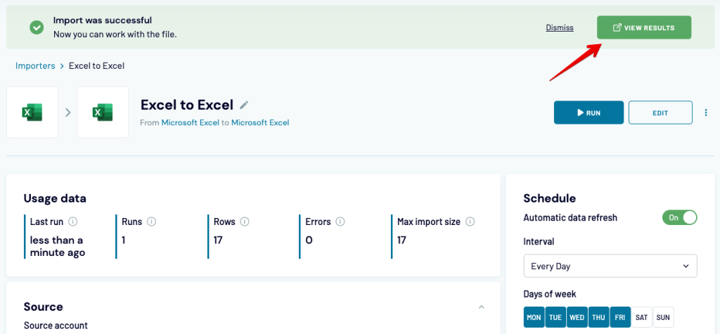
Finally, you can create a schedule for when the data should be imported. Choose what works best for you and run the importer.

Give it a little while to load, and then open the destination worksheet to see the results.
How to link Excel files and sync in real-time?
One of the advantages of using Excel files stored on OneDrive is their ability to sync data between one another. Microsoft advertises it as real-time sync but after some tests, we would call it a near real time.
If you’re used to the refresh rate of Google Sheets, for example, you may be disappointed. However, in most situations, a slight delay won’t cause any trouble.
To link files in Excel, follow the steps we outlined in the How to link Excel files chapter.
When data is changed in the destination file, most likely you won’t see an update visible right away in the source file. If you do nothing about it and just move on to the next task, you should see a refreshed number in a cell in a few minutes’ time. It will then continue refreshing at regular intervals.
If you want to speed things up, you can run an instant refresh by clicking Data -> Workbook Links in the menu and then the icon to refresh the data from a particular workbook.

This will often work, but only if the data in the source workbook has already been saved. Once again, it doesn’t happen instantly but only at regular (quite frequent) intervals.
If you’re anxious to have the data refreshed presently, you may consider refreshing the source file after making a change. This will prompt an automatic save. After that, manually force a data refresh in the destination file and it will fetch the latest saved data.
As a reminder, if you use Coupler.io to import data from one Excel workbook to another, you decide on the refresh schedule. For some, morning sync from Monday to Friday will do just fine. Others will prefer more frequent syncs – with Coupler.io you can even do it every 15 minutes.
FAQ: How to link Excel files
Let’s now discuss some specific use cases for how to link files in Excel. The tips below apply for files stored in OneDrive. If you only use Excel locally, jump back to the How to link local files in Excel section.
How to link cells in different Excel files?
For linking individual cells across files, the procedure is very much the same as we discussed earlier:
- Highlight the cell you want to reuse elsewhere and copy it.
- Right-click on the desired destination and select the Link icon from the Paste Options section.
If you’re importing to the same workbook as before, you won’t need to Enable Content again. If you reloaded it in the meantime, or are just linking the data to a new workbook, choose Manage Workbook Links and then Enable Content from the same bar.
Note that if you link multiple sets of cells or data ranges from the same workbook serving as a Source, they will all appear as a single position on your list of Workbook Links.
In the example below, you can see the data we imported from our sample Shopify store using Coupler.io.
We have a range of prices to the left linked from the respective workbook. Below there’s also a name of one of our products linked from another place in the same workbook. To the right, we can refresh data for all linked fields or, for example, enable automatic data refreshes.

How to link two Excel files without opening the source file?
You can link files in Excel without actually opening the source file. Of course, you’ll need to know the exact location of the cell or range of cells you wish to link. What’s more, to link Excel Online files or anything else stored on your OneDrive, you’ll need to fetch your unique ID.
To do so, set up a link in the traditional way we described above. Then, click on any linked cell in the Destination file and check its formula. It will look something like this:
='https://d.docs.live.net/18644c626caae38c/[myworkbook1.xlsx]Sheet1'!$C$2
The ID will follow right after the live.net link:

To insert a link from any given workbook, copy the formula with your ID and swap the file name and the cell range with the right values. Press ENTER and the latest data will be fetched.
How to link Excel columns between files?
Choosing a range of cells limits you to only the values currently present in the Source workbook. If anything new appears, it won’t be linked and, as such, won’t appear in the Destination workbook.
The solution is often to link an entire column and reference it in another file. To do so, click on any column in the Source file and copy it.
Then, select the first row of a column you want to add a link to and choose the Link icon. All the rows from the chosen column will be imported.

Rather than click, you can also enter the formulas directly. To link an entire column, it’s best to link to the first cell and then stretch the formula to the other rows.
When you insert the formula for the first row, be sure to remove the second $ (dollar) sign pointing to the specific cell. So, instead of the reference:
(...)Sheet1'!$C$2
Make it:
(...)Sheet1'!$C2
How to link fields between multiple files in Excel?
Advanced calculations may require referencing data from multiple spreadsheets at the same time. In the same way, the calculated data can then be referenced in other workbooks, creating a complex network of interconnected links.
As you recall from the earlier chapters, the formulas for linking cells between Excel Online files look somewhat like this:
='https://d.docs.live.net/18373e637ca3e48c/[Shopify Products - prices.xlsx]Sheet1'!$C$8
For the purpose of running any calculations or just adjusting the formulas as we go, the link is far too complex. It’s much better to link the desired fields into the destination workbook and then reference them from another worksheet in the same workbook.
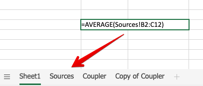
To do so, create a separate worksheet in your destination file where you’ll link all the external data. Name it accordingly – for example, “Sources”. Link the desired data by copying it from the source file and then pasting it as links (just as we did before).
Then, jump to the worksheet in the destination file. To reference the data from another sheet, use the following pattern:
Sheet_name!$A$1
For example, for calculating the average value of a range of cells present now in another worksheet, we would use:
=AVERAGE(Sources!B2:B12)
You can also type in the “=” sign (plus optionally a function name) and then jump to another worksheet and highlight the arguments. Press ENTER and the formula will be resolved.
In the standard version of Excel, the approach is pretty much the same, just with some small changes in the syntax of the links, as we mentioned earlier.
How to link Excel files – summing up
Linking Excel files can save you plenty of time and help you automate many dull processes.
It can also make things harder if you begin to link from one file to another, then to another, and another. The more interconnected workbooks become, the more complex it will be to troubleshoot the entire flow.
Find the right balance and use the right methods for linking your data.
When moving individual cells or ranges of them, Workbook Links work perfectly and are very easy to set up.
For moving large sets of data between workbooks or linking entire files, it’s a lot better to use tools such as Coupler.io. You’ll be able to set up your own schedule for imports, and all data transfers will happen outside of Excel. As a result, no Excel resources will be used, and you’ll be able to work much more smoothly while the information is synced in the background.
Thanks for reading!
-

Technical Content Writer on Coupler.io who loves working with data, writing about it, and even producing videos about it. I’ve worked at startups and product companies, writing content for technical audiences of all sorts. You’ll often see me cycling🚴🏼♂️, backpacking around the world🌎, and playing heavy board games.

Back to Blog
Focus on your business
goals while we take care of your data!
Try Coupler.io
Working with a lot of data can be a daunting task. However, knowing a few hacks and tricks can be useful for someone who is dealing with extensive data in Excel on a daily basis. One great example is how to link cells, worksheets, or workbooks in Excel. Linking in Excel will save you time and help you have more polished spreadsheets.
There are different ways to link cells in Excel. In this tutorial, we are going to cover certain aspects of the matter, including several solutions and methods.
The two main ways of linking cells in Excel are:
- External reference formula (Link)
- Excel hyperlink function
It is important to note that hyperlinks and external references are both very useful forms of linking different worksheets or workbooks; nevertheless, they have different purposes or uses. Here, we intend to focus on the external reference in more detail.
Linking Cells Between Sheets and Workbooks in Excel: External Reference
In Excel, you can basically use an external reference formula to refer to the content of cells on a worksheet in another workbook. This is also called linking, which is a more commonly used term. In other words, linking is referencing to:
- Another cell
- Range of cells
- A defined name
But, why is referencing useful, and how does it save time and effort?
Why Link Cells in Excel
Linking cells in Excel is beneficial when you have large volumes of data, and it is impractical to keep large worksheets in the same workbook.
Merging data
- You can use external references to integrate relevant data into a summary workbook.
- You can link several workbooks which belong to different members of the team or different departments.
- Once the source workbooks are changed, you won’t need to manually change the summary worksheet.
Giving different views of data
- You can generate a report workbook containing links to only the pertinent data.
- You can have all your other data on other source workbooks.
Organize large complex models
- You organize a complicated model by breaking it down into multiple interdependent workbooks.
- You can work on any of the sheets without opening all the related sheets.
- You can have smaller workbooks which are easier to manage.
- Smaller workbooks need less memory. They are faster to open, save and calculate
Linking Cells in Different Worksheets
Let’s start with the most basic form of external reference, which is to create a link to another worksheet (Tab) in the same workbook. Follow these steps:
- Select the cell where you want to create the link.
- Type an equal sign ‘=’.

- Go to the other worksheet that contains the cell you want to link to.
- Select the cell that you want to link to, and press Enter.
- Excel will automatically return to the original worksheet and display the value of the cell you selected.


Note: If you make any changes to the figures in the original worksheet, the value will be automatically updated in the target sheet.
What does the path represent? In this example, =Sheet2!D5, Sheet2 is the number of the sheet, and D5 is the cell that’s been linked to. The exclamation ‘!’ mark acts as a separator.
Linking a Range of Cells Using a Function
In this part, we are going to see how we can link a range of cells between worksheets in Excel. In other words, we are referencing data from a different worksheet. This is particularly useful when you have a large volume of data and want to have the results in another worksheet.
In our example, we have sales volume by quarter. We want to get the averages of sale volume for 2018, 2019, and 2020; however, we don’t want to display any of the raw data. So, we open a separate worksheet or tab. Now, follow these steps:

- Select the cell where you want to display the average.
- Type in the AVERAGE formula. Start with an equal sign, then type in AVERAGE and then open parentheses like so:
=average (
Related post: How to Calculate Average in Excel
- Now, go to the original sheet containing the raw data by clicking on the sheet tab. We want the data for 2018. So, select the data or the range of cells you want, and press ENTER to complete the path.
- When you press ENTER, Excel takes you back to the sheet where you entered the formula. And it’s going to have all the formulas there.
Note: As you can see, the formula includes the name of the sheet.
This is the formula: =AVARAGE(Sheet2!D2:D5) - We will do the same for the rest of the data, and this is the result.


Linking to a Defined Name in Another Workbook
This time we want to link different workbooks instead of worksheets. Our aim is to create an external reference to a defined name in another workbook.
Here, we have a workbook that contains budget data, and it is defined as Budget. Let’s quickly go through how to define a name in Excel. If you’re familiar with the process, skip this part.
Creating an Excel Name Range
- Select the range of cells you want to name.
- Type the name in the Name Box.
- Press, Enter.

Now, let’s go through the steps to link two different workbooks. Follow these instructions to create an external reference to a defined name in another workbook.
- Open the workbook containing the Budget data and the workbook that will contain the external reference.
- Select the cell or a range of cells you want to link to.
- Type = (equal sign).
- Switch to the other workbook and the sheet with the data you want to link. To do this: Go to View in the Menu bar. Then, find the Switch Windows option. When you click on it, you’ll notice a list of all the open workbooks. Select the workbook you want to pull data from.
- Press F3, the Paste Name window will pop up. Select the name you want to link, click OK, and press ENTER.
- Excel will automatically return to the other workbook and display the values from the range you selected.


Voila! This is how you can link two different workbooks with no sweat.
Bottom Line
In this tutorial, we covered 3 different methods, linking cells between sheets, linking a range of cells using the Average Function, and linking to a defined name in another workbook. The essential element here is the Equal sign ‘=.’ Every path you create for external referencing starts with an = (equal sign).
Did you find this tutorial useful? If so, check out our blogs and youtube channel. We offer customized Microsoft Excel solutions for businesses. If you find yourself backlogged and doing the same task over and over again, we are here to help. Our Excel programmers and consultant can automate and minimize your task.
FAQ
How do I link data from one Excel sheet to another?
You can simply type in = (equal sign) in a cell. Then click on the sheet, select the cell or range of cells you want and press enter. If you are familiar with formulas or paths, you can directly type the formula.
What is the Average formula?
Average is calculated by adding a group of numbers and then dividing the total sum by the total number of items. The Average formulas used in Excel are:
=AVERAGE(number1, [number2], …) …
=AVERAGE(B2:B11)
What are links in Excel?
External reference or a more commonly used term ‘linking’ is when you use, display or pull in data that is stored in another cell, worksheet, or even workbook. In other words, by creating external references, you can access the content of cells in another workbook, sheet, etc.