What is kurtosis in excel

This article describes the formula syntax and usage of the KURT function in Microsoft Excel.

Description

Returns the kurtosis of a data set. Kurtosis characterizes the relative peakedness or flatness of a distribution compared with the normal distribution. Positive kurtosis indicates a relatively peaked distribution. Negative kurtosis indicates a relatively flat distribution.

Syntax

KURT(number1, [number2], …)

The KURT function syntax has the following arguments:

• Number1, number2, …    Number1 is required, subsequent numbers are optional. 1 to 255 arguments for which you want to calculate kurtosis. You can also use a single array or a reference to an array instead of arguments separated by commas.

Remarks

• Arguments can either be numbers or names, arrays, or references that contain numbers.

• Logical values and text representations of numbers that you type directly into the list of arguments are counted.

• If an array or reference argument contains text, logical values, or empty cells, those values are ignored; however, cells with the value zero are included.

• Arguments that are error values or text that cannot be translated into numbers cause errors.

• If there are fewer than four data points, or if the standard deviation of the sample equals zero, KURT returns the #DIV/0! error value.

• Kurtosis is defined as:

  

  where s is the sample standard deviation.

Example

Copy the example data in the following table, and paste it in cell A1 of a new Excel worksheet. For formulas to show results, select them, press F2, and then press Enter. If you need to, you can adjust the column widths to see all the data.

Data
3
4
5
2
3
4
5
6
4
7
Formula	Description	Result
=KURT(A2:A11)	Kurtosis of the data set above	-0.151799637

Updated on March 06, 2017

Kurtosis is a descriptive statistic that is not as well known as other descriptive statistics such as the mean and standard deviation. Descriptive statistics give some sort of summary information about a data set or distribution. As the mean is a measurement of the center of a data set and the standard deviation how spread out the data set is, kurtosis is a measurement of the thickness of the fails of a distribution.

The formula for kurtosis can be somewhat tedious to use, as it involves several intermediate calculations. However, statistical software greatly speeds up the process of calculating kurtosis. We will see how to calculate kurtosis with Excel.

Types of Kurtosis

Before seeing how to calculate kurtosis with Excel, we will examine a few key definitions. If the kurtosis of a distribution is greater than that of a normal distribution, then it has positive excess kurtosis and is said to be leptokurtic. If a distribution has kurtosis that is less than a normal distribution, then it has negative excess kurtosis and is said to be platykurtic. Sometimes the words kurtosis and excess kurtosis are used interchangeably, so be sure to know which one of these calculations you want.

Kurtosis in Excel

With Excel it is very straightforward to calculate kurtosis. Performing the following steps streamlines the process of using the formula displayed above.  Excel’s kurtosis function calculates excess kurtosis.

1. Enter the data values into cells.
2. In a new cell type =KURT(
3. Highlight the cells where the data are at. Or type the range of cells containing the data.
4. Make sure to close the parentheses by typing )
5. Then press the enter key.

The value in the cell is the excess kurtosis of the data set.

For smaller data sets, there is an alternate strategy that will work:

1. In an empty cell type =KURT(
2. Enter the data values, each separated by a comma.
3. Close the parentheses with )
4. Press the enter key.

This method is not as preferable because the data are hidden within the function, and we cannot do other calculations, such as a standard deviation or mean, with the data that we have entered.

Limitations

It is also important to note that Excel is limited by the amount of data that the kurtosis function, KURT, can handle. The maximum number of data values that can be used with this function is 255.

Due to the fact that the function contains the quantities (n — 1), (n — 2) and (n — 3) in the denominator of a fraction, we must have a data set of at least four values in order to use this Excel function. For data sets of size 1, 2 or 3, we would have a division by zero error. We also must have a nonzero standard deviation in order to avoid a division by zero error.

When the data is plotted in the form of a histogram it exhibits a degree of peakedness or flatness. The degree of peakedness or flatness of the data can be measured by calculating kurtosis.

How to Find Kurtosis in Excel:

Step 1: Open a new worksheet. Input the raw data values into the cells. For example, we input the data in columns B, C, D, and E in the example below.

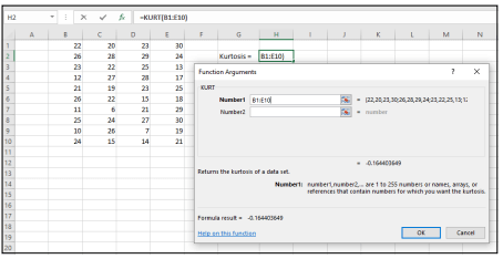
Step 2: Go to the statistical functions menu. Choose the KURT function in order to open the KURT function argument dialog box.

Step 3: Choose the cells where you have inputted the data values. Also, select a cell where you can obtain the output.

Step 4: Click on OK in order to obtain the value of the excess kurtosis as the output on the selected cell.

Hey 👋

I have always been passionate about statistics and mathematics education.

I created this website to explain mathematical and statistical concepts in the simplest possible manner.

If you’ve found value from reading my content, feel free to support me in even the smallest way you can.

KURT Excel Function

In Excel, kurtosis can be comfortably calculated using the KURT Excel function. The only argument needed for KURT function is the range of cells containing the data.

For example the formula:

=KURT(C5:C104)

… calculates kurtosis for the set of values contained in cells C5 through C104.

Which Kind of Kurtosis Excel Actually Calculates

The KURT Excel function calculates sample excess kurtosis – it is this formula:

If you want to use Excel for calculating one of the other kinds of kurtosis – sample kurtosis, population kurtosis, or population excess kurtosis, there is no built-in Excel function you can simply use. You can either calculate them by adjusting from the KURT Excel function, or calculate them directly from your input data. See the rest of this page for details.

For differences in the four kinds of kurtosis and detailed explanation of the formulas, see kurtosis formula.

Calculating Population Excess Kurtosis in Excel

You can calculate population excess kurtosis directly using this formula:

One disadvantage of this calculation is that you need to calculate the individual deviations from the mean, squared and raised to the power of 4, in separate cells. If you are working with large data sets, it will make the Excel file very big and possibly slow to calculate.

Therefore it is often better to use the KURT Excel function and adjust the result from sample to population. The adjustment is as follows:

=((KURT(Data!$B$16:$B$10015)*($G$5-2)*($G$5-3)/($G$5-1))-6)/($G$5+1)

This is the function I use in the Descriptive Statistics Calculator. The first part — KURT(Data!$B$16:$B$10015) – is the built-in Excel KURT function for sample excess kurtosis of cells B16 through B10015, and the rest is the adjustment from sample to population excess kurtosis, where cell G5 calculates population size:

=COUNT(Data!$B$16:$B$10015)

The whole formula is:

Population Excess Kurtosis = ( ( Sample Excess Kurtosis · (n – 2) (n – 3) / (n – 1) ) – 6 ) / (n + 1)

… where n = population size (number of values)

As you can see, you don’t need to calculate the deviations from the mean in separate cells.

Calculating Population Kurtosis in Excel

If you want to calculate population (non-excess) kurtosis in Excel, you simply take population excess kurtosis that we’ve just calculated above and add 3, because:

Population Excess Kurtosis = Population Kurtosis – 3

Calculating Sample Kurtosis in Excel

Contrary to popular belief, sample excess kurtosis does not equal sample kurtosis less 3 (as it is with population kurtosis), but you need to adjust the minus 3 for the data set being a sample.

Sample excess kurtosis is:

Sample kurtosis is:

Therefore you can calculate sample kurtosis from sample excess kurtosis (which is the direct result of the built-in KURT Excel function) as follows:

Sample Kurtosis = Sample Excess Kurtosis + ( 3 (n – 1)² / ( (n – 2) (n – 3) ) )

If you don’t mind a large Excel file you can also calculate sample kurtosis directly using the sample kurtosis formula above.

You can see how kurtosis Excel calculation works in practice in the Descriptive Statistics Calculator.

Steps of Descriptive Statistics With Excel

1. Go to Data >> data analysis.
2. You’ll see many statistical options there, choose descriptive statistics >> ok.
3. In the popup window, you have several fields that you have to fill. Input range: block the data you want to analyze.
4. Click Ok.
5. See the magic happens!

How do you report the results of descriptive statistics?

When reporting descriptive statistic from a variable you should, at a minimum, report a measure of central tendency and a measure of variability. In most cases, this includes the mean and reporting the standard deviation (see below). In APA format you do not use the same symbols as statistical formulas.

How do you analyze descriptive data?

Steps to do descriptive analysis:

1. Step 1: Draw out your objectives.
2. Step 2: Collect your data.
3. Step 3: Clean your data.
4. Step 4: Data analysis.
5. Step 5: Interpret the results.
6. Step 6: Communicating Results.

How do you interpret kurtosis in descriptive statistics?

If the kurtosis is greater than 3, then the dataset has heavier tails than a normal distribution (more in the tails). If the kurtosis is less than 3, then the dataset has lighter tails than a normal distribution (less in the tails).

How do you interpret standard deviation and descriptive statistics?

That is, how data is spread out from the mean. A low standard deviation indicates that the data points tend to be close to the mean of the data set, while a high standard deviation indicates that the data points are spread out over a wider range of values.

Excel Descriptive Statistics
Using the descriptive statistics feature in Excel means that you won’t have to type in individual functions like MEAN or MODE. One button click will return a dozen different stats for your data set.

How do you interpret statistical significance?

The level of statistical significance is often expressed as a p-value between 0 and 1. The smaller the p-value, the stronger the evidence that you should reject the null hypothesis. A p-value less than 0.05 (typically ≤ 0.05) is statistically significant.

What are the 5 descriptive statistics?

There are a variety of descriptive statistics. Numbers such as the mean, median, mode, skewness, kurtosis, standard deviation, first quartile and third quartile, to name a few, each tell us something about our data.

How do you interpret kurtosis in Excel?

When interpreting kurtosis, the normal distribution is used a reference. A positive kurtosis implies a distribution with more extreme possible data values (outliers) than a normal distribution thus fatter tails (Leptokurtic distributions).

How do you interpret skewness and kurtosis in descriptive statistics?

A general guideline for skewness is that if the number is greater than +1 or lower than –1, this is an indication of a substantially skewed distribution. For kurtosis, the general guideline is that if the number is greater than +1, the distribution is too peaked.

How do you interpret skewness and kurtosis values?

For skewness, if the value is greater than + 1.0, the distribution is right skewed. If the value is less than -1.0, the distribution is left skewed. For kurtosis, if the value is greater than + 1.0, the distribution is leptokurtik. If the value is less than -1.0, the distribution is platykurtik.

How do you interpret the range in descriptive statistics?

Interpretation. Use the range to understand the amount of dispersion in the data. A large range value indicates greater dispersion in the data. A small range value indicates that there is less dispersion in the data.

How do you analyze descriptive statistics in SPSS?

Steps of Descriptive Statistics on SPSS

1. Choose Analyze > Descriptive Statistics >> Frequencies.
2. Move the variables that we want to analyze.
3. On the right side of the submenu, you will see three options you could add; statistics, chart, and format.
4. You can do another descriptive analysis on this menu.
5. Click Ok.

What is descriptive statistics explain with the help of example?

Descriptive statistics are used to describe or summarize data in ways that are meaningful and useful. For example, it would not be useful to know that all of the participants in our example wore blue shoes. However, it would be useful to know how spread out their anxiety ratings were.

How do you Analyse data in Excel?

Simply select a cell in a data range > select the Analyze Data button on the Home tab. Analyze Data in Excel will analyze your data, and return interesting visuals about it in a task pane.

How do you summarize data in Excel?

Select the column to summarize on

1. With a cell selected in an Add-In for Excel table, click the ACL Add-In tab and select Summarize > Summarize.
2. Select a column of any data type to summarize on.
3. Optional To omit the count or percentage for the unique values in the column, clear Include count or Include percentage.

What is the meaning of 0.05 level of significance?

5%
The significance level, also denoted as alpha or α, is the probability of rejecting the null hypothesis when it is true. For example, a significance level of 0.05 indicates a 5% risk of concluding that a difference exists when there is no actual difference.

What z score is significant?

The probability of randomly selecting a score between -1.96 and +1.96 standard deviations from the mean is 95% (see Fig. 4). If there is less than a 5% chance of a raw score being selected randomly, then this is a statistically significant result.

Is p 0.1 statistically significant?

If the p-value is under . 01, results are considered statistically significant and if it’s below . 005 they are considered highly statistically significant.

What are the 4 types of descriptive statistics?

There are four major types of descriptive statistics:

• Measures of Frequency: * Count, Percent, Frequency.
• Measures of Central Tendency. * Mean, Median, and Mode.
• Measures of Dispersion or Variation. * Range, Variance, Standard Deviation.
• Measures of Position. * Percentile Ranks, Quartile Ranks.

What are the 8 descriptive statistics?

In this article, the first one, you’ll find the usual descriptive statistics concepts: Measures of Central Tendency: Mean, Median, Mode. Measures of Dispersion: Variance and Standard Deviation. Measures of Position: Quartiles, Quantiles and Interquartiles.

In this Excel tutorial, you will learn how to calculate a Kuthosis in Excel.

What is the Kurthosis?

Kurtosis is a measure of the concentration of results. Kurtosis informs us about how our observations and the results are concentrated around the mean. This measure tells us how much of your results or observations are close to the average, or how many of the observed results have a value similar to the average.

Kurtosis determines the strength of the extreme value instrument, so it measures what happens in the «tails» of the classification. Contrary to what is stated, alien to some textbooks, kurtosis does not measure the «flattening», «slenderness» and «pointedness» of the distribution.

Probability distributions can be divided according to the value of kurtosis into the following distributions:

• mesokurtic — the kurtosis value is 0, the flattening of the distribution is similar to the flattening of a normal distribution (for which the kurtosis is exactly 0)
• leptokurtic — kurtosis is positive, trait values are more concentrated than with normal distribution
• platykurtic — kurtosis is negative, trait values are less concentrated than with normal distribution

Syntax

KURT (number1, number2, …)

Number 1, number2, … are the arguments 1 through 255 for which the kurtosis is calculated. A single array or an array reference can be used in place of arguments separated by commas. If there are fewer than four data points, or if the sample standard deviation is zero, KURT returns #DIV / 0! Error value.

The calculation of kurtosis is possible, but you initially need data such as this:

How to calculate?

You should click on an empty cell (1), and type =KURT(all the cells, ex. A1:A10) (2), then press enter.

Kurt Excel function has been used here.

Investors often use kurtosis as it provides information about the risk and rate of return on their investment. High rate of return kurtosis increases the likelihood of achieving a higher rate of return on investment. Thus, investors are willing to pay more for investments with a leptokurtic schedule than for investments with a platykurtic schedule. Knowing the actual distribution of the rate of return on a given investment allows you to better manage the investor’s risk and portfolio, and also allows you to construct a range in which the investor can expect a rate of return.

The KURT function will return the kurtosis of your data set. Note that the KURT function calculates the excess kurtosis, which is the kurtosis of a set of values minus 3. A kurtosis value of 3 represents a normal distribution, and values greater than 3 indicate a distribution with a heavier tail than a normal distribution.

In addition to the KURT function, you can also calculate the kurtosis of your data set using the following formula:

=SUM((A2:A11-AVERAGE(A2:A11))^4)/COUNT(A2:A11)/(STDEV(A2:A11)^4) — 3

Replace the range A2:A11 with the range of cells that contains your data. The formula will return the excess kurtosis of your data set.

You can download a free Kurtosis Calculator template here.

Рассмотрим инструмент Описательная статистика, входящий в надстройку Пакет Анализа. Рассчитаем показатели выборки: среднее, медиана, мода, дисперсия, стандартное отклонение и др.

Задача

описательной статистики

(descriptive statistics) заключается в том, чтобы с использованием математических инструментов свести сотни значений

выборки

к нескольким итоговым показателям, которые дают представление о

выборке

.В качестве таких статистических показателей используются:

среднее

,

медиана

,

мода

,

дисперсия, стандартное отклонение

и др.

Опишем набор числовых данных с помощью определенных показателей. Для чего нужны эти показатели? Эти показатели позволят сделать определенные

статистические выводы о распределении

, из которого была взята

выборка

. Например, если у нас есть

выборка

значений толщины трубы, которая изготавливается на определенном оборудовании, то на основании анализа этой

выборки

мы сможем сделать, с некой определенной вероятностью, заключение о состоянии процесса изготовления.

Содержание статьи:

• Надстройка Пакет анализа;
• Среднее выборки

  ;

• Медиана выборки

  ;

• Мода выборки

  ;

• Мода и среднее значение

  ;

• Дисперсия выборки

  ;

• Стандартное отклонение выборки

  ;

• Стандартная ошибка

  ;

• Ассиметричность

  ;

• Эксцесс выборки

  ;

• Уровень надежности

  .

Надстройка Пакет анализа

Для вычисления статистических показателей одномерных

выборок

, используем

надстройку Пакет анализа

. Затем, все показатели рассчитанные надстройкой, вычислим с помощью встроенных функций MS EXCEL.

СОВЕТ

: Подробнее о других инструментах надстройки

Пакет анализа

и ее подключении – читайте в статье

Надстройка Пакет анализа MS EXCEL

.

Выборку

разместим на

листе

Пример

в файле примера

в диапазоне

А6:А55

(50 значений).

Примечание

: Для удобства написания формул для диапазона

А6:А55

создан

Именованный диапазон

Выборка.

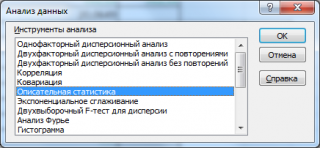
В диалоговом окне

Анализ данных

выберите инструмент

Описательная статистика

.

После нажатия кнопки

ОК

будет выведено другое диалоговое окно,

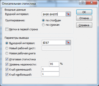
в котором нужно указать:

• 
  входной интервал
  
  (Input Range) – это диапазон ячеек, в котором содержится массив данных. Если в указанный диапазон входит текстовый заголовок набора данных, то нужно поставить галочку в поле
  
  Метки в первой строке (
  
  Labels
  
  in
  
  first
  
  row
  
  ).
  
  В этом случае заголовок будет выведен в
  
  Выходном интервале.
  
  Пустые ячейки будут проигнорированы, поэтому нулевые значения необходимо обязательно указывать в ячейках, а не оставлять их пустыми;
• 
  выходной интервал
  
  (Output Range). Здесь укажите адрес верхней левой ячейки диапазона, в который будут выведены статистические показатели;
• 
  Итоговая статистика (
  
  Summary
  
  Statistics
  
  )
  
  . Поставьте галочку напротив этого поля – будут выведены основные показатели выборки:
  
  среднее, медиана, мода, стандартное отклонение
  
  и др.;
• Также можно поставить галочки напротив полей
  
  Уровень надежности (
  
  Confidence
  
  Level
  
  for
  
  Mean
  
  )
  
  ,
  
  К-й наименьший
  
  (Kth Largest) и
  
  К-й наибольший
  
  (Kth Smallest).

В результате будут выведены следующие статистические показатели:

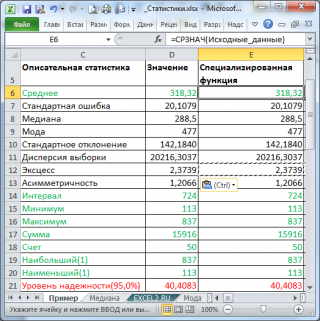
Все показатели выведены в виде значений, а не формул. Если массив данных изменился, то необходимо перезапустить расчет.

Если во

входном интервале

указать ссылку на несколько столбцов данных, то будет рассчитано соответствующее количество наборов показателей. Такой подход позволяет сравнить несколько наборов данных. При сравнении нескольких наборов данных используйте заголовки (включите их во

Входной интервал

и установите галочку в поле

Метки в первой строке

). Если наборы данных разной длины, то это не проблема — пустые ячейки будут проигнорированы.

Зеленым цветом на картинке выше и в

файле примера

выделены показатели, которые не требуют особого пояснения. Для большинства из них имеется специализированная функция:

• 
  Интервал
  
  (Range) — разница между максимальным и минимальным  значениями;
• 
  Минимум
  
  (Minimum) – минимальное значение в диапазоне ячеек, указанном во
  
  Входном интервале
  
  (см.

  статью про функцию
  
  МИН()
  
  );

• 
  Максимум
  
  (Maximum)– максимальное значение (см.

  статью про функцию
  
  МАКС()
  
  );

• 
  Сумма
  
  (Sum) – сумма всех значений (см.

  статью про функцию
  
  СУММ()
  
  );

• 
  Счет
  
  (Count) – количество значений во
  
  Входном интервале
  
  (пустые ячейки игнорируются, см.

  статью про функцию
  
  СЧЁТ()
  
  );

• 
  Наибольший
  
  (Kth Largest) – выводится К-й наибольший. Например, 1-й наибольший – это максимальное значение (см.

  статью про функцию
  
  НАИБОЛЬШИЙ()
  
  );

• 
  Наименьший
  
  (Kth Smallest) – выводится К-й наименьший. Например, 1-й наименьший – это минимальное значение (см.

  статью про функцию
  
  НАИМЕНЬШИЙ()
  
  ).

Ниже даны подробные описания остальных показателей.

Среднее выборки

Среднее

(mean, average) или

выборочное среднее

или

среднее выборки

(sample average) представляет собой

арифметическое среднее

всех значений массива. В MS EXCEL для вычисления среднего выборки используется функция

СРЗНАЧ()

.

Выборочное среднее

является «хорошей» (несмещенной и эффективной) оценкой

математического ожидания

случайной величины (подробнее см. статью

Среднее и Математическое ожидание в MS EXCEL

).

Медиана выборки

Медиана

(Median) – это число, которое является серединой множества чисел (в данном случае выборки): половина чисел множества больше, чем

медиана

, а половина чисел меньше, чем

медиана

. Для определения

медианы

необходимо сначала

отсортировать множество чисел

. Например,

медианой

для чисел 2, 3, 3,

4

, 5, 7, 10 будет 4.

Если множество содержит четное количество чисел, то вычисляется

среднее

для двух чисел, находящихся в середине множества. Например,

медианой

для чисел 2, 3,

3

,

5

, 7, 10 будет 4, т.к. (3+5)/2.

Если имеется длинный хвост распределения, то

Медиана

лучше, чем

среднее значение

, отражает «типичное» или «центральное» значение. Например, рассмотрим несправедливое распределение зарплат в компании, в которой руководство получает существенно больше, чем основная масса сотрудников.

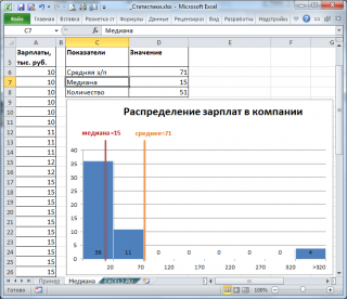
Очевидно, что средняя зарплата (71 тыс. руб.) не отражает тот факт, что 86% сотрудников получает не более 30 тыс. руб. (т.е. 86% сотрудников получает зарплату в более, чем в 2 раза меньше средней!). В то же время медиана (15 тыс. руб.) показывает, что

как минимум

у 50% сотрудников зарплата меньше или равна 15 тыс. руб.

Для определения

медианы

в MS EXCEL существует одноименная функция

МЕДИАНА()

, английский вариант — MEDIAN().

Медиану

также можно вычислить с помощью формул

=КВАРТИЛЬ.ВКЛ(Выборка;2) =ПРОЦЕНТИЛЬ.ВКЛ(Выборка;0,5).

Подробнее о

медиане

см. специальную статью

Медиана в MS EXCEL

.

СОВЕТ

: Подробнее про

квартили

см. статью, про

перцентили (процентили)

см. статью.

Мода выборки

Мода

(Mode) – это наиболее часто встречающееся (повторяющееся) значение в

выборке

. Например, в массиве (1; 1;

2

;

2

;

2

; 3; 4; 5) число 2 встречается чаще всего – 3 раза. Значит, число 2 – это

мода

. Для вычисления

моды

используется функция

МОДА()

, английский вариант MODE().

Примечание

: Если в массиве нет повторяющихся значений, то функция вернет значение ошибки #Н/Д. Это свойство использовано в статье

Есть ли повторы в списке?

Начиная с

MS EXCEL 2010

вместо функции

МОДА()

рекомендуется использовать функцию

МОДА.ОДН()

, которая является ее полным аналогом. Кроме того, в MS EXCEL 2010 появилась новая функция

МОДА.НСК()

, которая возвращает несколько наиболее часто повторяющихся значений (если количество их повторов совпадает). НСК – это сокращение от слова НеСКолько.

Например, в массиве (1; 1;

2

;

2

;

2

; 3;

4

;

4

;

4

; 5) числа 2 и 4 встречаются наиболее часто – по 3 раза. Значит, оба числа являются

модами

. Функции

МОДА.ОДН()

и

МОДА()

вернут значение 2, т.к. 2 встречается первым, среди наиболее повторяющихся значений (см.

файл примера

, лист

Мода

).

Чтобы исправить эту несправедливость и была введена функция

МОДА.НСК()

, которая выводит все

моды

. Для этого ее нужно ввести как

формулу массива

.

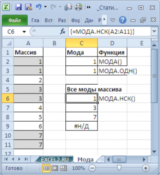
Как видно из картинки выше, функция

МОДА.НСК()

вернула все три

моды

из массива чисел в диапазоне

A2:A11

: 1; 3 и 7. Для этого, выделите диапазон

C6:C9

, в

Строку формул

введите формулу

=МОДА.НСК(A2:A11)

и нажмите

CTRL+SHIFT+ENTER

. Диапазон

C

6:

C

9

охватывает 4 ячейки, т.е. количество выделяемых ячеек должно быть больше или равно количеству

мод

. Если ячеек больше чем м

о

д, то избыточные ячейки будут заполнены значениями ошибки #Н/Д. Если

мода

только одна, то все выделенные ячейки будут заполнены значением этой

моды

.

Теперь вспомним, что мы определили

моду

для выборки, т.е. для конечного множества значений, взятых из

генеральной совокупности

. Для

непрерывных случайных величин

вполне может оказаться, что выборка состоит из массива на подобие этого (0,935; 1,211; 2,430; 3,668; 3,874; …), в котором может не оказаться повторов и функция

МОДА()

вернет ошибку.

Даже в нашем массиве с

модой

, которая была определена с помощью

надстройки Пакет анализа

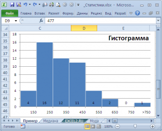
, творится, что-то не то. Действительно,

модой

нашего массива значений является число 477, т.к. оно встречается 2 раза, остальные значения не повторяются. Но, если мы посмотрим на

гистограмму распределения

, построенную для нашего массива, то увидим, что 477 не принадлежит интервалу наиболее часто встречающихся значений (от 150 до 250).

Проблема в том, что мы определили

моду

как наиболее часто встречающееся значение, а не как наиболее вероятное. Поэтому,

моду

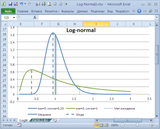
в учебниках статистики часто определяют не для выборки (массива), а для функции распределения. Например, для

логнормального распределения

мода

(наиболее вероятное значение непрерывной случайной величины х), вычисляется как

exp

(

m

—

s

²

)

, где m и s параметры этого распределения.

Понятно, что для нашего массива число 477, хотя и является наиболее часто повторяющимся значением, но все же является плохой оценкой для

моды

распределения, из которого взята

выборка

(наиболее вероятного значения или для которого плотность вероятности распределения максимальна).

Для того, чтобы получить оценку

моды

распределения, из

генеральной совокупности

которого взята

выборка

, можно, например, построить

гистограмму

. Оценкой для

моды

может служить интервал наиболее часто встречающихся значений (самого высокого столбца). Как было сказано выше, в нашем случае это интервал от 150 до 250.

Вывод

: Значение

моды

для

выборки

, рассчитанное с помощью функции

МОДА()

, может ввести в заблуждение, особенно для небольших выборок. Эта функция эффективна, когда случайная величина может принимать лишь несколько дискретных значений, а размер

выборки

существенно превышает количество этих значений.

Например, в рассмотренном примере о распределении заработных плат (см. раздел статьи выше, о Медиане),

модой

является число 15 (17 значений из 51, т.е. 33%). В этом случае функция

МОДА()

дает хорошую оценку «наиболее вероятного» значения зарплаты.

Примечание

: Строго говоря, в примере с зарплатой мы имеем дело скорее с

генеральной совокупностью

, чем с

выборкой

. Т.к. других зарплат в компании просто нет.

О вычислении

моды

для распределения

непрерывной случайной величины

читайте статью

Мода в MS EXCEL

.

Мода и среднее значение

Не смотря на то, что

мода

– это наиболее вероятное значение случайной величины (вероятность выбрать это значение из

Генеральной совокупности

максимальна), не следует ожидать, что

среднее значение

обязательно будет близко к

моде

.

Примечание

:

Мода

и

среднее

симметричных распределений совпадает (имеется ввиду симметричность

плотности распределения

).

Представим, что мы бросаем некий «неправильный» кубик, у которого на гранях имеются значения (1; 2; 3; 4; 6; 6), т.е. значения 5 нет, а есть вторая 6.

Модой

является 6, а среднее значение – 3,6666.

Другой пример. Для

Логнормального распределения

LnN(0;1)

мода

равна =EXP(m-s2)= EXP(0-1*1)=0,368, а

среднее значение

1,649.

Дисперсия выборки

Дисперсия выборки

или

выборочная дисперсия (

sample

variance

) характеризует разброс значений в массиве, отклонение от

среднего

.

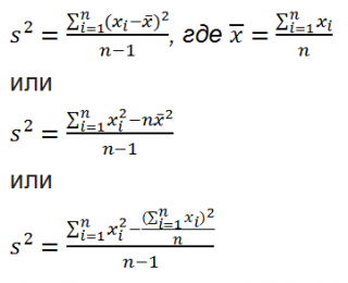
Из формулы №1 видно, что

дисперсия выборки

это сумма квадратов отклонений каждого значения в массиве

от среднего

, деленная на размер выборки минус 1.

В MS EXCEL 2007 и более ранних версиях для вычисления

дисперсии выборки

используется функция

ДИСП()

. С версии MS EXCEL 2010 рекомендуется использовать ее аналог — функцию

ДИСП.В()

.

Дисперсию

можно также вычислить непосредственно по нижеуказанным формулам (см.

файл примера

):

=КВАДРОТКЛ(Выборка)/(СЧЁТ(Выборка)-1) =(СУММКВ(Выборка)-СЧЁТ(Выборка)*СРЗНАЧ(Выборка)^2)/ (СЧЁТ(Выборка)-1)

– обычная формула

=СУММ((Выборка -СРЗНАЧ(Выборка))^2)/ (СЧЁТ(Выборка)-1)

–

формула массива

Дисперсия выборки

равна 0, только в том случае, если все значения равны между собой и, соответственно, равны

среднему значению

.

Чем больше величина

дисперсии

, тем больше разброс значений в массиве относительно

среднего

.

Размерность

дисперсии

соответствует квадрату единицы измерения исходных значений. Например, если значения в выборке представляют собой измерения веса детали (в кг), то размерность

дисперсии

будет кг

²

. Это бывает сложно интерпретировать, поэтому для характеристики разброса значений чаще используют величину равную квадратному корню из

дисперсии – стандартное отклонение

.

Подробнее о

дисперсии

см. статью

Дисперсия и стандартное отклонение в MS EXCEL

.

Стандартное отклонение выборки

Стандартное отклонение выборки

(Standard Deviation), как и

дисперсия

, — это мера того, насколько широко разбросаны значения в выборке

относительно их среднего

.

По определению,

стандартное отклонение

равно квадратному корню из

дисперсии

:

Стандартное отклонение

не учитывает величину значений в

выборке

, а только степень рассеивания значений вокруг их

среднего

. Чтобы проиллюстрировать это приведем пример.

Вычислим стандартное отклонение для 2-х

выборок

: (1; 5; 9) и (1001; 1005; 1009). В обоих случаях, s=4. Очевидно, что отношение величины стандартного отклонения к значениям массива у

выборок

существенно отличается.

В MS EXCEL 2007 и более ранних версиях для вычисления

Стандартного отклонения выборки

используется функция

СТАНДОТКЛОН()

. С версии MS EXCEL 2010 рекомендуется использовать ее аналог

СТАНДОТКЛОН.В()

.

Стандартное отклонение

можно также вычислить непосредственно по нижеуказанным формулам (см.

файл примера

):

=КОРЕНЬ(КВАДРОТКЛ(Выборка)/(СЧЁТ(Выборка)-1)) =КОРЕНЬ((СУММКВ(Выборка)-СЧЁТ(Выборка)*СРЗНАЧ(Выборка)^2)/(СЧЁТ(Выборка)-1))

Подробнее о

стандартном отклонении

см. статью

Дисперсия и стандартное отклонение в MS EXCEL

.

Стандартная ошибка

В

Пакете анализа

под термином

стандартная ошибка

имеется ввиду

Стандартная ошибка среднего

(Standard Error of the Mean, SEM).

Стандартная ошибка среднего

— это оценка

стандартного отклонения

распределения

выборочного среднего

.

Примечание

: Чтобы разобраться с понятием

Стандартная ошибка среднего

необходимо прочитать о

выборочном распределении

(см. статью

Статистики, их выборочные распределения и точечные оценки параметров распределений в MS EXCEL

) и статью про

Центральную предельную теорему

.

Стандартное отклонение распределения выборочного среднего

вычисляется по формуле σ/√n, где n — объём

выборки, σ — стандартное отклонение исходного

распределения, из которого взята

выборка

. Т.к. обычно

стандартное отклонение

исходного распределения неизвестно, то в расчетах вместо

σ

используют ее оценку

s

—

стандартное отклонение выборки

. А соответствующая величина s/√n имеет специальное название —

Стандартная ошибка среднего.

Именно эта величина вычисляется в

Пакете анализа.

В MS EXCEL

стандартную ошибку среднего

можно также вычислить по формуле

=СТАНДОТКЛОН.В(Выборка)/ КОРЕНЬ(СЧЁТ(Выборка))

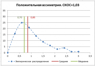
Асимметричность

Асимметричность

или

коэффициент асимметрии

(skewness) характеризует степень несимметричности распределения (

плотности распределения

) относительно его

среднего

.

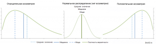
Положительное значение

коэффициента асимметрии

указывает, что размер правого «хвоста» распределения больше, чем левого (относительно среднего). Отрицательная асимметрия, наоборот, указывает на то, что левый хвост распределения больше правого.

Коэффициент асимметрии

идеально симметричного распределения или выборки равно 0.

Примечание

:

Асимметрия выборки

может отличаться расчетного значения асимметрии теоретического распределения. Например,

Нормальное распределение

является симметричным распределением (

плотность его распределения

симметрична относительно

среднего

) и, поэтому имеет асимметрию равную 0. Понятно, что при этом значения в

выборке

из соответствующей

генеральной совокупности

не обязательно должны располагаться совершенно симметрично относительно

среднего

. Поэтому,

асимметрия выборки

, являющейся оценкой

асимметрии распределения

, может отличаться от 0.

Функция

СКОС()

, английский вариант SKEW(), возвращает коэффициент

асимметрии выборки

, являющейся оценкой

асимметрии

соответствующего распределения, и определяется следующим образом:

где n – размер

выборки

, s –

стандартное отклонение выборки

.

В

файле примера на листе СКОС

приведен расчет коэффициента

асимметрии

на примере случайной выборки из

распределения Вейбулла

, которое имеет значительную положительную

асимметрию

при параметрах распределения W(1,5; 1).

Эксцесс выборки

Эксцесс

показывает относительный вес «хвостов» распределения относительно его центральной части.

Для того чтобы определить, что относится к хвостам распределения, а что к его центральной части, можно использовать границы μ +/-

σ

.

Примечание

: Не смотря на старания профессиональных статистиков, в литературе еще попадается определение

Эксцесса

как меры «остроконечности» (peakedness) или сглаженности распределения. Но, на самом деле, значение

Эксцесса

ничего не говорит о форме пика распределения.

Согласно определения,

Эксцесс

равен четвертому

стандартизированному моменту:

Для

нормального распределения

четвертый момент равен 3*σ

⁴

, следовательно,

Эксцесс

равен 3. Многие компьютерные программы используют для расчетов не сам

Эксцесс

, а так называемый Kurtosis excess, который меньше на 3. Т.е. для

нормального распределения

Kurtosis excess равен 0. Необходимо быть внимательным, т.к. часто не очевидно, какая формула лежит в основе расчетов.

Примечание

: Еще большую путаницу вносит перевод этих терминов на русский язык. Термин Kurtosis происходит от греческого слова «изогнутый», «имеющий арку». Так сложилось, что на русский язык оба термина Kurtosis и Kurtosis excess переводятся как

Эксцесс

(от англ. excess — «излишек»). Например, функция MS EXCEL

ЭКСЦЕСС()

на самом деле вычисляет Kurtosis excess.

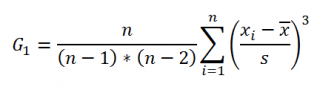
Функция

ЭКСЦЕСС()

, английский вариант KURT(), вычисляет на основе значений выборки несмещенную оценку

эксцесса распределения

случайной величины и определяется следующим образом:

Как видно из формулы MS EXCEL использует именно Kurtosis excess, т.е. для выборки из

нормального распределения

формула вернет близкое к 0 значение.

Если задано менее четырех точек данных, то функция

ЭКСЦЕСС()

возвращает значение ошибки #ДЕЛ/0!

Вернемся к

распределениям случайной величины

.

Эксцесс

(Kurtosis excess) для

нормального распределения

всегда равен 0, т.е. не зависит от параметров распределения μ и σ. Для большинства других распределений

Эксцесс

зависит от параметров распределения: см., например,

распределение Вейбулла

или

распределение Пуассона

, для котрого

Эксцесс

= 1/λ.

Уровень надежности

Уровень

надежности

— означает вероятность того, что

доверительный интервал

содержит истинное значение оцениваемого параметра распределения.

Вместо термина

Уровень

надежности

часто используется термин

Уровень доверия

. Про

Уровень надежности

(Confidence Level for Mean) читайте статью

Уровень значимости и уровень надежности в MS EXCEL

.

Задав значение

Уровня

надежности

в окне

надстройки Пакет анализа

, MS EXCEL вычислит половину ширины

доверительного интервала для оценки среднего (дисперсия неизвестна)

.

Тот же результат можно получить по формуле (см.

файл примера

):

=ДОВЕРИТ.СТЬЮДЕНТ(1-0,95;s;n)

s —

стандартное отклонение выборки

, n – объем

выборки

.

Подробнее см. статью про

построение доверительного интервала для оценки среднего (дисперсия неизвестна)

.