
Excel for Microsoft 365 Excel for Microsoft 365 for Mac Excel for the web Excel 2021 Excel 2021 for Mac Excel 2019 Excel 2019 for Mac Excel 2016 Excel 2016 for Mac Excel 2013 Excel 2010 Excel 2007 Excel for Mac 2011 Excel Starter 2010 More…Less
This article describes the formula syntax and usage of the INT function in Microsoft Excel.
Description
Rounds a number down to the nearest integer.
Syntax
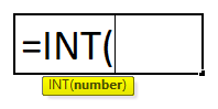
INT(number)
The INT function syntax has the following arguments:
-
Number Required. The real number you want to round down to an integer.
Example
Copy the example data in the following table, and paste it in cell A1 of a new Excel worksheet. For formulas to show results, select them, press F2, and then press Enter. If you need to, you can adjust the column widths to see all the data.
|
Data |
||
|---|---|---|
|
19.5 |
||
|
Formula |
Description |
Result |
|
=INT(8.9) |
Rounds 8.9 down |
8 |
|
=INT(-8.9) |
Rounds -8.9 down. Rounding a negative number down rounds it away from 0. |
-9 |
|
=A2-INT(A2) |
Returns the decimal part of a positive real number in cell A2 |
0.5 |
Need more help?
What is INT (Integer) Function in Excel?
The INT Excel function rounds a decimal number down to the nearest integer and returns it. It is one of the rounding functions in Excel which returns a positive or negative integer as an output. However, it returns the nearest lower integer in the case of positive numbers, and the negative numbers become more negative.
For example, below, we have two numbers. Let us apply the INT formula to them and check the output. Enter the formula =INT(A2) in cell B2. Press Enter and copy the formula to B3 as well. The INT function returns the integer 3 for the number 3.6. When we use the function on -3.6, it returns an integer away from zero, that is, -4.

Table of contents
- What is INT(Integer) Function in Excel?
- INT() Excel Formula
- How to Use INT(Integer) Excel Function?
- Entering INT Excel Function Manually
- Access from the Excel Ribbon
- Examples
- Example #1
- Example #2
- Example #3
- Important Things to Note
- Frequently Asked Questions (FAQs)
- Download Template
- Recommended Articles
- The INT Excel function rounds any number to the nearest lower integer in the case of positive numbers. It removes the decimal part of a number.
- In the case of negative numbers, the INT Excel function returns the nearest decimal number away from zero. Hence, the number becomes more negative. Using the MOD and INT excel functions, we can separate a number as an integer and decimal part.
- It is one of the rounding functions in Excel. The other rounding functions are TRUNC, ROUND, EVEN, etc.
INT() Excel Formula
The syntax of the INT Excel function is as follows:

Arguments
Number (mandatory) – This is the number that you want to round to the nearest integer.
How to Use INT(Integer) Excel Function?
The INT Excel function is one of the most used rounding functions. It is very similar to TRUNC excel function. Now, we can use INT() in two ways. First, it can be entered manually or selected from the Formulas tab in the Excel ribbon.
Entering INT Excel Function Manually
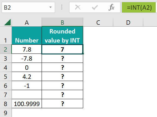
Below is a list of numbers for which you must find the nearest integer value.

- Place the cursor in cell B2 to find the nearest integer of the number 7.8.
- Enter the formula as follows: =INT(A2) and press Enter.

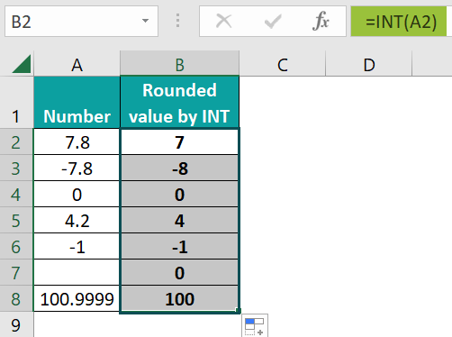
- You get result 7 for argument 7.8. In the case of positive numbers, the function returns the lower nearest integer. Now, drag the Autofill handle from A2 to A8.
• As observed in the results, you can see that in the case of negative numbers like -7.8, the output is the nearest integer, which is away from zero, that is, -8.
• Also, when the number is already an integer like -1(cell A6), the output is the same number.
• For a blank cell like A7, the output obtained is zero.
• Even if the number is 100.9999(cell A8), it is not rounded off to 101 but to 100.
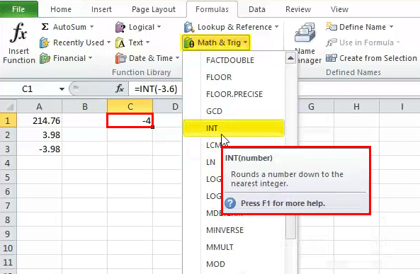
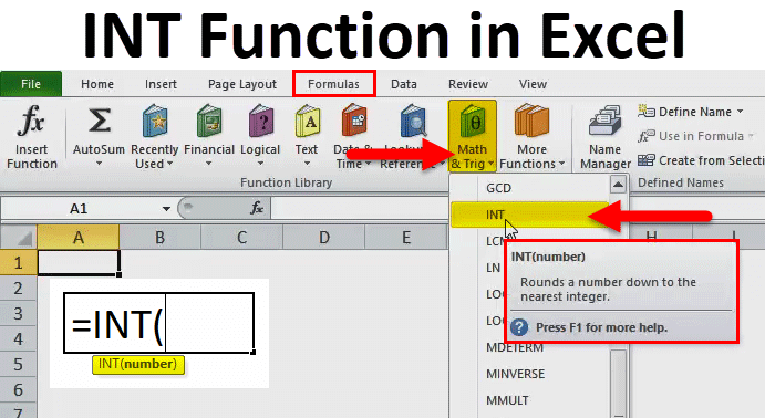
Access from the Excel Ribbon
- Step 1: Choose an empty cell to get the output.
- Step 2: Go to the Formulas tab and click on the Math & Trig Drop Down arrow.
- Step 3: You get all the functions under this category. Select the INT function.

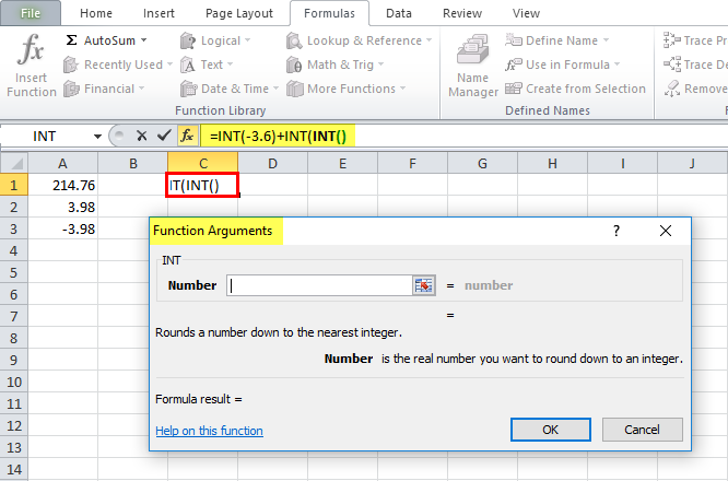
- Step 4: A pop-up window appears. Enter the “Number to get the nearest integer of that number.

Thus, the INT Excel function can be accessed in two ways, manually or through the Excel ribbon, as seen above.
Examples
If you are left wondering about the use of the INT function in Excel, as it is simple, you can look at some examples below to understand its importance.
Example #1
Below is a set of different values. Let us apply the INT function to each number and check the outcome. Let us also compare it with a similar function in Excel, TRUNC. Like INT, the TRUNC Excel function removes the decimal part of a number and gives us just the integer part.
However, it is slightly different from the INT Excel function, which we will observe below.

- Step 1: Apply the function =INT(C4) in cell D4, to get the nearest integer for 156.54. Apply the function =TRUNC(C4) in cell E4.


- Step 2: You can observe that both the INT and TRUNC functions have given the same output, 156.
Here, TRUNC has removed the decimal part of 156.54, while INT has rounded the number to the nearest lower integer, 156. Drag the Autofill excel handles in cells D4 and E4 up to cells D10 and E10, respectively.

Let us observe each result.
- 184.00 has been rounded off to 184 by both functions.
- INT has rounded off -254.5 to the nearest integer away from zero, -255, while the decimal part has been removed by TRUNC, thereby producing a different output, -254.
- Similarly, in the case of -2.9, INT gives the nearest integer away from zero, -3, while TRUNC removes the decimal and provides an output of -2.
- A non-numeric value gives an #VALUE! error for both functions.
- Both the INT and TRUNC functions supply a numeric value for the time value 12:00:00 AM. It is because Excel stores the time as a serial number. Therefore, you must format both the cells as Time in the Number group to obtain the time.
Example #2
In this INT excel function example, we have date and time information in cells B2 to B8. Here, we must separate the time and date. The INT formula helps us separate the time and date with precision.

- Step 1: Excel stores Date as an integer, while Time is stored as a decimal fraction. To obtain only the date from Column B, you must get the integer part of the cell.
- Step 2: Enter =INT(B2) in cell C2. Press Enter. You get the integer part of cell B2, that is, the date.

- Step 3: Drag the Autofill handle up to cell C8. You get the date for all the cells.

- Step 4: You must get the time part alone from Column B. It’s simple! Just subtract the integer part obtained in Column C from the whole date and time in Column B.
Apply the formula =B2-C2 in cell D2 and press Enter.

- Step 5: Copy the formula from D2 to D8 by dragging the Autofill handle. You can find the time information in Column D. You can format Columns C and D as Date and Time, respectively, using the Numbers group of the Home tab.

Example #3
In this example, we have a list of employees who have served an organization. Their date of joining and date of leaving details have been provided. We must find the number of days each employee worked for the organization. We must also find the information on exact days and years’ count.

- Step 1: First, we must find the number of days the employee has worked. Since dates are stored as integers in Excel, you must subtract the joining date from the date of leaving.
Type the formula =INT(D3) – INT(C3) in cell E3. Press Enter. You get the number of days the first employee, Sam, worked for the organization.

- Step 2: Drag the handle from E3 to E13 to get the details on the number of days all the employees have worked for the organization.

- Step 3: To find the total duration the employees have worked in terms of years and days, you may use the functions INT and MOD. While INT gives you the integer part, which is the years’ count when you divide the total days by 365; MOD gives you the remainder, which represents the remaining days.
Apply the following function to cell F3 and press Enter.
=INT(E3/365)&” Years “&MOD(E3,365)&” Days”
Here,
- When you divide the days in Column E by 365, you get the number of years the employee has worked for the company.
- When you use MOD after dividing by 365, you get the days remaining after obtaining the years. MOD takes two arguments, MOD(number, divisor), and returns the remainder.
- ‘&’ is used to concatenate the different strings and operators.

- Step 4: Drag the handle from F3 to F13 to get the number of days and years each employee has worked.

Thus, the INT function returns the nearest integer for any value and can be used in various ways.
Important Things to Note
- If the argument to the INT function is a text, we will get the #VALUE! Error in Microsoft Excel. However, if an integer is stored as a string, to convert string to INT excel function, you should use the VALUE excel function.
- If the excel cell reference supplied to the INT function is invalid, it will return a #REF! Error, and you will observe the INT excel function not working.
- INT() belongs to the class Math and Trig functions in Excel.
- For positive numbers, INT and TRUNC give the same output; however, INT returns an integer away from zero for negative numbers, while TRUNC removes the decimal part.
Frequently Asked Questions (FAQs)
1. What does INT function do in Excel?
The INT Excel function returns the integer part of a decimal number. It also returns the nearest integer, lower than the number supplied. In the case of negative numbers, it returns the nearest integer away from zero. For instance, =INT(-3.5) gives an output of -4.
2. How do you format INT in Excel?
When any number is entered in an Excel cell, it is in the General format. However, if you convert it into the nearest integer using the INT Excel function, you can format it according to requirements, such as a number, date, etc., by right-clicking and choosing the Format Cells option. Then, select the Number tab in the pop-up window and format the INT function.
3. How do you round up to an INT in Excel?
If you have a decimal number, you can round it up to the nearest integer with several rounding functions available in Excel. Also, you can use the INT or TRUNC function to round a number to the nearest integer. The other rounding functions include ROUND, ODD, EVEN, and so on.
Download Template
This article must help understand INT Excel Function with its formula and examples. You can download the template here to use it instantly.
Recommended Articles
A guide to INT Excel Function and its definition. Here we learn how to use INTEGER formula along with examples and downloadable excel template. You can learn more from the following articles –
- ISODD Excel Function
- EVEN Function in Excel
- ROUND Excel Function
Содержание
- INT function in Excel
- What is INT function in Excel?
- How to use INT function in excel
- Examples of INT function in excel
- How to use INT function in excel
- What is the purpose of INT function?
- What is the Return value of INT function?
- How many arguments does INTfunction have?
- Which version of excel supports INT function?
- INT Function
- Related functions
- Summary
- Purpose
- Return value
- Arguments
- Syntax
- Usage notes
- Examples
- INT vs. TRUNC
- Rounding functions in Excel
- INT Excel Function (Integer)
- INT Function in Excel
- Formula
- Parameters
- Return Value
- Usage Notes
- How to Open the Integer Function in Excel?
- All Rounding Functions in Excel (Including INT)
- Functions Used to Round a Number to an Integer Value
- Functions Used to Round a Number to a Specified Number of Decimal Places
- Functions Used to Round a Number to a Supplied Multiple of Significance(MS)
- How to Use INT in Excel?
- Example #1
- Example #2
- Example #3
- Example #4
- Applications
- INT Excel Function Errors
- Things to Remember
- Recommended Articles
- Excel INT Function
- What is the Excel INT Function?
- INT Syntax
- How to Use INT Function in Excel
- INT Function #1 – INT Function #3
- INT Function #4 – INT Function #6
- INT Function #7 – INT Function #9
INT function in Excel
What is INT function in Excel?
The INT function is one of the math functions of Excel.
It Rounds a number down to a Nearest integer.
We can find this function in Math & trig of insert function Tab.
How to use INT function in excel
- Click on an empty cell (like F5 )

2. Click on the fx icon (or press shift+F3)

3. In the insert function tab you will see all functions

4. Select math and trig category
5. Select INT function
6. Then select ok

7. In the function Arguments Tab you will see the INT function
8. In the number section you can enter the value to round (for example 1.5)
9. If you enter +1.5 result will be 1

10. If you enter 2.5 result will be 2

11. If you enter -1.5 result will be -2

12. If you enter -2.5 result will be -3

13. You will see results in the formula result section
Examples of INT function in excel
Example 1:
How to use INT function in excel
You can see examples of INT function below:

What is the purpose of INT function?
It Rounds a number down to a Nearest integer.
What is the Return value of INT function?
It returns a number.
How many arguments does INT function have?
This function has just 1 Argument.
The argument of INT function is number.
In the number section you can enter the value to round (for example 1.5).
The argument of INT function is required and not optional.
Which version of excel supports INT function?
This function is available for all excel versions (2003-2019)
Источник
INT Function

Summary
The Excel INT function returns the integer part of a decimal number by rounding down to the integer. Note that negative numbers become more negative. For example, while INT(10.8) returns 10, INT(-10.8) returns -11.
Purpose
Return value
Arguments
- number — The number from which you want an integer.
Syntax
Usage notes
The INT function returns the integer part of a decimal number by rounding down to the integer. It is important to understand that the INT function returns the integer part of a decimal number, after rounding down. One consequence of this behavior is that negative numbers become more negative. For example, while INT(10.8) returns 10, INT(-10.8) returns -11. To return an integer by truncating decimals, see the TRUNC function.
The INT function takes just one argument, number, which should be a numeric value. INT returns a #VALUE! error if number is not a numeric value. If number is already a whole number, INT has no effect.
Examples
When numbers are positive, the INT function rounds down to the next lowest whole number:
Notice INT rounds positive numbers down toward zero. With negative numbers, INT rounds down away from zero:
INT vs. TRUNC
INT is similar to the TRUNC function because they both can return the integer part of a number. However, TRUNC simply truncates a number, while INT actually rounds a number down to an integer. With positive numbers, and when TRUNC is using the default of 0 for num_digits, both functions return the same results. With negative numbers, the results can be different. INT(-3.1) returns -4, because INT rounds down to the lower integer. TRUNC(-3.1) returns -3. If you simply want the integer part of a number, you should use TRUNC.
Rounding functions in Excel
Excel provides a number of functions for rounding:
- To round normally, use the ROUND function.
- To round to the nearest multiple, use the MROUND function.
- To round down to the nearest specified place, use the ROUNDDOWN function.
- To round down to the nearest specified multiple, use the FLOOR function.
- To round up to the nearest specified place, use the ROUNDUP function.
- To round up to the nearest specified multiple, use the CEILING function.
- To round down and return an integer only, use the INT function.
- To truncate decimal places, use the TRUNC function.
Источник
INT Excel Function (Integer)


INT Function in Excel
INT or Integer function in Excel returns the nearest integer of a given number. This function is used when we have a large number of data sets. Each data is in a different format. For example, float, this function returns the integer part of the number.
The Microsoft Excel INT function is a function that is responsible for returning the integer portion of a number. It works by rounding down a decimal number to an integer. It is a built-in Excel function. It is categorized as a Math & Trig Function in Excel. It is used either as a worksheet function or a VBA function Worksheet Function Or A VBA Function The worksheet function in VBA is used when we need to refer to a specific worksheet. When we create a module, the code runs in the currently active sheet of the workbook, but we can use the worksheet function to run the code in a particular worksheet. read more . It can be entered as a part of the INT formula, a cell of a worksheet. Here, negative numbers become more negative because the function rounds down. For example, INT (10.6) returns 10 and INT (-10.6) returns -11.
Table of contents
Formula

Parameters
It accepts the following parameters and arguments:
number – The number to be entered from which you want an integer.
Return Value
The return value will be a numeric integer.
Usage Notes
- It can be used when you want only the integer part of a number in its decimal form with rounding the number down. For example, INT (3.89) returns the value 3.
- The integer function always rounds down the number entered in the formula to the next lowest integer value.
- We can also use the TRUNC function in excelTRUNC Function In ExcelTrunc is an excel function to minimize decimal numbers to integers. TRUNC eliminates the fractional part of decimal and returns only the integer part under the required precision. It was first introduced in the excel 2007.read more to get the integer part of both negative and positive numbers.
How to Open the Integer Function in Excel?
Below are the steps to open integer function in excel –
- First, we can insert the desired integer Excel formula in the required cell to attain a return value on the argument.
We can manually open the INT formula dialog box in the spreadsheet and enter the logical values to attain a return value.
Consider the screenshot below to see the INT Function in the excel option under the Math & Trig Function menu.
Click on the INT function option. The INT formula in the excel dialogue box may open where we can put the argument values to obtain a return value.
All Rounding Functions in Excel (Including INT)
Consider the three tables below, which specify each function and its behavior.
Please note that in the below-given tables, “more” is depicted by “+,” and less is depicted by “-.”
Functions Used to Round a Number to an Integer Value

Functions Used to Round a Number to a Specified Number of Decimal Places

Functions Used to Round a Number to a Supplied Multiple of Significance(MS)

How to Use INT in Excel?
Excel INT function is very simple and easy to use. Let us look below at some of the examples of the INT function in Excel. These examples will help you explore the use of the INT function in Excel.


Consider the below screenshots of the above integer function in Excel examples.
Example #1
We must apply the INT formula =INT(A1) to get 214.

Example #2
We must apply the INT formula in Excel =INT(A2) to get 3.

Example #3
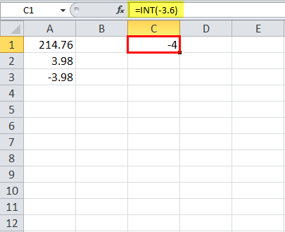
We must apply the INT Excel function here: =INT(A3) to get -4.

Example #4
Using the formula =INT(-3.6) to get -4.
Applications
Here are a few examples where it is generally used.
- Extracting dates from a date and timetable
- Cash denomination calculator
- Getting age from birthday
- Rounding a number to ‘n’ significant digits
- Getting days, hours, and minutes between dates
- Calculating years between dates
- Getting the integer part of a number
INT Excel Function Errors
If we get any error from the INT Excel function, then it can be any one of the following:
- #NAME? – This error occurs when Excel does not recognize the text in the formula. For example, we may have entered the wrong text in the function’s syntax.
- #VALUE! – If we enter the wrong type of argument in the syntax of the function, we will be getting this error in Microsoft ExcelError In Microsoft ExcelErrors in excel are common and often occur at times of applying formulas. The list of nine most common excel errors are — #DIV/0, #N/A, #NAME?, #NULL!, #NUM!, #REF!, #VALUE!, #####, Circular Reference.read more .
- #REF! – Microsoft Excel will display this error if the formula refers to a cell that is not valid.
Things to Remember
- It returns the integer position of the number.
- It rounds down the decimal number to its integer.
- It is categorized under the “Math & Trig” function.
- Suppose we use the Integer function; negative numbers become more negative because it rounds down the number. For example, INT (10.6) returns 10 and INT (-10.6) returns -11.
Recommended Articles
This article is a guide to INT Function in Excel. Here, we discuss the Integer formula in Excel and how to use it in Excel, along with an Excel example and downloadable Excel templates. You may also look at these useful functions in Excel: –
Источник
Excel INT Function
What is the Excel INT Function?
The excel INT function is not used to get an integer number from a number, for a positive number, it’s correct, but for a negative number, it’s wrong.
The excel INT function is used to round down all numbers, to the nearest integer. For a positive number, will get an integer number equal to the original number, but for a negative number, will get a more negative number, not the same as the original number.
Use the excel TRUNC function to get the same integer number as the original number, whether it’s a positive or a negative number.
INT Syntax
number, required, the number you want to round down to the nearest integer.
How to Use INT Function in Excel
For example, there are numbers like the picture below. What is the result if the number in column A is used as a “number” argument of the INT function?
INT Function #1 – INT Function #3
For a positive number regardless of number, whether there are fractions or not, always return the same integer number as the origin, because the INT function rounds down to the nearest integer number.
INT Function #4 – INT Function #6
For negative numbers, no matter the number of fractions, always get an integer number that is different from the origin. Why? The INT function rounds down, if the number is negative, it will become more negative and different from the original number.
For negative numbers, the INT function returns the same integer number as the origin if there are no fractional numbers.
INT Function #7 – INT Function #9
Although in excel documentation a “number” argument must be a number, it turns out that if it’s filled with alphanumeric (the number represented as text), it doesn’t matter. As long excel successfully converts it to a number, Excel will round down to the nearest integer number.
If Excel unsuccessfully to convert, it returns a #VALUE! error.
See the picture below for the results of the nine INT functions.
Источник
How to Use Excel > Excel Functions > Excel INT Function
How to Use the Excel INT Function
Table of contents :
- What is the Excel INT Function?
- INT Syntax
- How to Use INT Function in Excel
- INT Example

What is the Excel INT Function?
The excel INT function is not used to get an integer number from a number, for a positive number, it’s correct, but for a negative number, it’s wrong.
The excel INT function is used to round down all numbers, to the nearest integer. For a positive number, will get an integer number equal to the original number, but for a negative number, will get a more negative number, not the same as the original number.
Use the excel TRUNC function to get the same integer number as the original number, whether it’s a positive or a negative number.
INT Syntax
INT(number)
number, required, the number you want to round down to the nearest integer.
How to Use INT Function in Excel
For example, there are numbers like the picture below. What is the result if the number in column A is used as a “number” argument of the INT function?

INT Function #1 – INT Function #3
=INT(A2)

=INT(A3)

=INT(A4)
For a positive number regardless of number, whether there are fractions or not, always return the same integer number as the origin, because the INT function rounds down to the nearest integer number.
INT Function #4 – INT Function #6
=INT(A5)

=INT(A6)

=INT(A7)
For negative numbers, no matter the number of fractions, always get an integer number that is different from the origin. Why? The INT function rounds down, if the number is negative, it will become more negative and different from the original number.
For negative numbers, the INT function returns the same integer number as the origin if there are no fractional numbers.
INT Function #7 – INT Function #9
=INT(A8)

=INT(A9)

=INT(A10)
Although in excel documentation a “number” argument must be a number, it turns out that if it’s filled with alphanumeric (the number represented as text), it doesn’t matter. As long excel successfully converts it to a number, Excel will round down to the nearest integer number.
If Excel unsuccessfully to convert, it returns a #VALUE! error.
See the picture below for the results of the nine INT functions.
INT Example
Another article using or explain about INT Function
Another Round Function
Another article about Round Function
INT or Integer function in Excel returns the nearest integer of a given number. This function is used when we have a large number of data sets. Each data is in a different format. For example, float, this function returns the integer part of the number.
The Microsoft Excel INT function is a function that is responsible for returning the integer portion of a number. It works by rounding down a decimal number to an integer. It is a built-in Excel function. It is categorized as a Math & Trig Function in Excel. It is used either as a worksheet function or a VBA functionThe worksheet function in VBA is used when we need to refer to a specific worksheet. When we create a module, the code runs in the currently active sheet of the workbook, but we can use the worksheet function to run the code in a particular worksheet.read more. It can be entered as a part of the INT formula, a cell of a worksheet. Here, negative numbers become more negative because the function rounds down. For example, INT (10.6) returns 10 and INT (-10.6) returns -11.
Table of contents
- INT Function in Excel
- Formula
- Parameters
- Return Value
- Usage Notes
- How to Open the Integer Function in Excel?
- All Rounding Functions in Excel (Including INT)
- Functions Used to Round a Number to an Integer Value
- Functions Used to Round a Number to a Specified Number of Decimal Places
- Functions Used to Round a Number to a Supplied Multiple of Significance(MS)
- How to Use INT in Excel?
- Example #1
- Example #2
- Example #3
- Example #4
- Applications
- INT Excel Function Errors
- Things to Remember
- Recommended Articles
Formula
Parameters
It accepts the following parameters and arguments:
number – The number to be entered from which you want an integer.
Return Value
The return value will be a numeric integer.
Usage Notes
- It can be used when you want only the integer part of a number in its decimal form with rounding the number down. For example, INT (3.89) returns the value 3.
- The integer function always rounds down the number entered in the formula to the next lowest integer value.
- We can also use the TRUNC function in excelTrunc is an excel function to minimize decimal numbers to integers. TRUNC eliminates the fractional part of decimal and returns only the integer part under the required precision. It was first introduced in the excel 2007.read more to get the integer part of both negative and positive numbers.
How to Open the Integer Function in Excel?
Below are the steps to open integer function in excel –
- First, we can insert the desired integer Excel formula in the required cell to attain a return value on the argument.
- We can manually open the INT formula dialog box in the spreadsheet and enter the logical values to attain a return value.
- Consider the screenshot below to see the INT Function in the excel option under the Math & Trig Function menu.

- Click on the INT function option. The INT formula in the excel dialogue box may open where we can put the argument values to obtain a return value.

All Rounding Functions in Excel (Including INT)
There are a total of fifteen rounding functions in ExcelROUND is a built-in Excel function that calculates the round number of a given number using the number of digits as an argument. The number to be rounded up to and the number of digits to be rounded up to are the two arguments to this formula.read more.
Consider the three tables below, which specify each function and its behavior.
Please note that in the below-given tables, “more” is depicted by “+,” and less is depicted by “-.”
Functions Used to Round a Number to an Integer Value
Functions Used to Round a Number to a Specified Number of Decimal Places
Functions Used to Round a Number to a Supplied Multiple of Significance(MS)
How to Use INT in Excel?
Excel INT function is very simple and easy to use. Let us look below at some of the examples of the INT function in Excel. These examples will help you explore the use of the INT function in Excel.
You can download this INT Function in Excel here – INT Function in Excel
Based on the above INT in the Excel spreadsheet, let us consider these examples and see the SUBTOTAL functionThe SUBTOTAL excel function performs different arithmetic operations like average, product, sum, standard deviation, variance etc., on a defined range.read more return based on the syntax of the INT formula in Excel.
Consider the below screenshots of the above integer function in Excel examples.
Example #1
We must apply the INT formula =INT(A1) to get 214.
Example #2
We must apply the INT formula in Excel =INT(A2) to get 3.
Example #3
We must apply the INT Excel function here: =INT(A3) to get -4.
Example #4
Using the formula =INT(-3.6) to get -4.
Applications
Here are a few examples where it is generally used.
- Extracting dates from a date and timetable
- Cash denomination calculator
- Getting age from birthday
- Rounding a number to ‘n’ significant digits
- Getting days, hours, and minutes between dates
- Calculating years between dates
- Getting the integer part of a number
INT Excel Function Errors
If we get any error from the INT Excel function, then it can be any one of the following:
- #NAME? – This error occurs when Excel does not recognize the text in the formula. For example, we may have entered the wrong text in the function’s syntax.
- #VALUE! – If we enter the wrong type of argument in the syntax of the function, we will be getting this error in Microsoft ExcelErrors in excel are common and often occur at times of applying formulas. The list of nine most common excel errors are — #DIV/0, #N/A, #NAME?, #NULL!, #NUM!, #REF!, #VALUE!, #####, Circular Reference.read more.
- #REF! – Microsoft Excel will display this error if the formula refers to a cell that is not valid.
Things to Remember
- It returns the integer position of the number.
- It rounds down the decimal number to its integer.
- It is categorized under the “Math & Trig” function.
- Suppose we use the Integer function; negative numbers become more negative because it rounds down the number. For example, INT (10.6) returns 10 and INT (-10.6) returns -11.
Recommended Articles
This article is a guide to INT Function in Excel. Here, we discuss the Integer formula in Excel and how to use it in Excel, along with an Excel example and downloadable Excel templates. You may also look at these useful functions in Excel: –
- VBA INT FunctionVBA INT is an inbuilt function used to give us only the integer part of a number provided with an input. This function helps in data whose decimal part is not affecting the data to ease the calculations or analysis with only the integer values.read more
- VBA IntegerIn VBA, an integer is a data type that may be assigned to any variable and used to hold integer values. In VBA, the bracket for the maximum number of integer variables that can be kept is similar to that in other languages. Using the DIM statement, any variable can be defined as an integer variable.read more
- SMALL Function in ExcelThe SMALL Function in Excel returns the nth smallest value from a set of values. For example, 2nd smallest value, 3rd smallest value and so on.read more
- ROUNDUP Function in ExcelThe ROUNDUP excel function calculates the rounded value of the number to the upward side or the higher side. In other words, it rounds the number away from zero. Being an inbuilt function of Excel, it accepts two arguments–the “number” and the “num_of _digits.” For example, “=ROUNDUP(0.40,1)” returns 0.4.
read more
Reader Interactions
Purpose
Get the integer part of a number by rounding down
Return value
The integer part of the number after rounding down
Usage notes
The INT function returns the integer part of a decimal number by rounding down to the integer. It is important to understand that the INT function returns the integer part of a decimal number, after rounding down. One consequence of this behavior is that negative numbers become more negative. For example, while INT(10.8) returns 10, INT(-10.8) returns -11. To return an integer by truncating decimals, see the TRUNC function.
The INT function takes just one argument, number, which should be a numeric value. INT returns a #VALUE! error if number is not a numeric value. If number is already a whole number, INT has no effect.
Examples
When numbers are positive, the INT function rounds down to the next lowest whole number:
=INT(3.25) // returns 3
=INT(3.99) // returns 3
=INT(3.01) // returns 3
Notice INT rounds positive numbers down toward zero. With negative numbers, INT rounds down away from zero:
=INT(-3.25) // returns -4
=INT(-3.99) // returns -4
=INT(-3.01) // returns -4
INT vs. TRUNC
INT is similar to the TRUNC function because they both can return the integer part of a number. However, TRUNC simply truncates a number, while INT actually rounds a number down to an integer. With positive numbers, and when TRUNC is using the default of 0 for num_digits, both functions return the same results. With negative numbers, the results can be different. INT(-3.1) returns -4, because INT rounds down to the lower integer. TRUNC(-3.1) returns -3. If you simply want the integer part of a number, you should use TRUNC.
Rounding functions in Excel
Excel provides a number of functions for rounding:
- To round normally, use the ROUND function.
- To round to the nearest multiple, use the MROUND function.
- To round down to the nearest specified place, use the ROUNDDOWN function.
- To round down to the nearest specified multiple, use the FLOOR function.
- To round up to the nearest specified place, use the ROUNDUP function.
- To round up to the nearest specified multiple, use the CEILING function.
- To round down and return an integer only, use the INT function.
- To truncate decimal places, use the TRUNC function.
Notes
- INT returns a #VALUE! error if number is not a numeric value.
- Use the INT function to get an integer from a number by rounding.
- Use the TRUNC function to return an integer by truncating.
INT Function in Excel (Table of Contents)
- INT in Excel
- How to use INT Function in Excel?
INT in Excel
Int function is a very simple function used to convert any number into an integer value. Integer values are any number which is a whole number, but it can be a positive number or negative number. Int function can consider any number, whether it is decimal, fraction, or square root value, but in the end, we will be getting a whole number out of it.
INT Formula in Excel:
Below is the INT Formula in Excel.
where
Number or Expression – It is the number you want to round down to the nearest integer.
How to Use INT Function in Excel?
INT function in Excel is very simple and easy to use. Let us understand the working of INT function in Excel by some INT Formula example. INT function can be used as a worksheet function and as a VBA function.
You can download this INT Function Excel Template here – INT Function Excel Template
Example #1
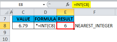
The below-mentioned table contains a value in cell “C8”, i.e. 6.79, which is a positive number; I need to find out the nearest integer for 6.79 using the INT function in Excel.
Select the cell “E8” where the INT function needs to be applied.
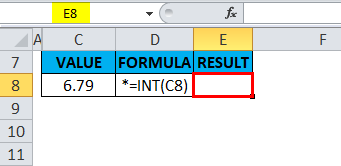
Click the insert function button (fx) under the formula toolbar; a dialog box will appear, type the keyword “INT” in the search for a function box, INT function will appear in select a function box. Double click on the INT function.
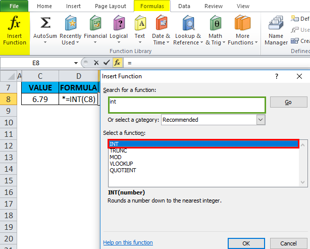
A dialog box appears where arguments (number) for the INT function need to be filled or entered.
i.e. =INT(C8).

It removes the decimal from the number and returns the integer part of the number, i.e. 6.
Example #2
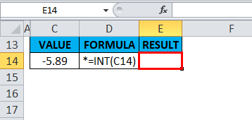
The below-mentioned table contains a value in cell “C14”, i.e. -5.89, which is a negative number; I need to find out the nearest integer for -5.89 using the INT function in Excel. Select the cell E14 where the INT function needs to be applied.
Click the insert function button (fx) under the formula toolbar; a dialog box will appear, type the keyword “INT” in the search for a function box, INT function will appear in select a function box. Double click on the INT function.
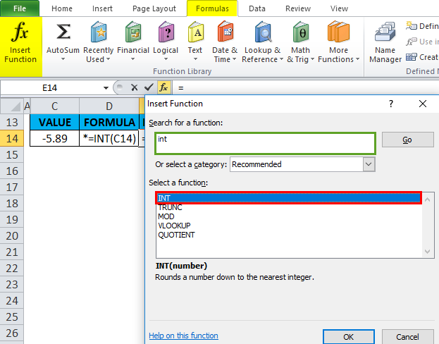
A dialog box appears where arguments (number) for the INT function need to be filled or entered.
i.e. =INT(C14)
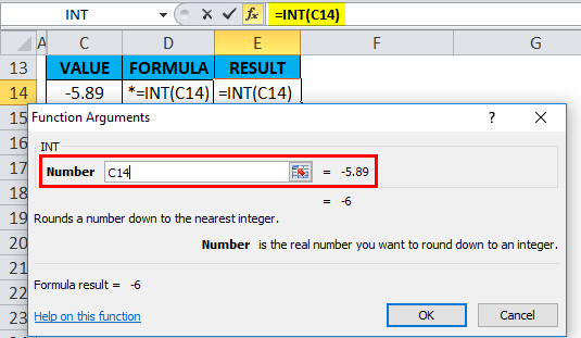
It removes the decimal from the number and returns the integer part of the number, i.e. -6.
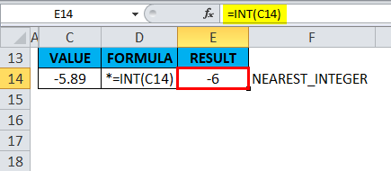
When the INT function is applied for a negative number, it rounds down the number. i.e. It returns the number which is lower than the given number (More negative value).
Example #3
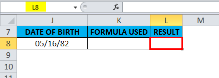
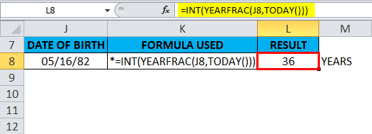
In the below mention example, I have the date of birth ( 16th May 1982) in the cell “J8” I need to calculate the age in cell “L8” using the INT function in Excel.
Prior to the INT function in Excel, let’s know about the YEARFRAC function; the YEARFRAC function returns a decimal value that represents fractional years between two dates. I.e. Syntax is =YEARFRAC (start_date, end_date, [basis]) it returns the number of days between 2 dates as a year.
Here the INT function is integrated with the YEARFRAC function in cell “L8”.
YEARFRAC formula takes the date of birth and the current date (which is given by the TODAY function), and it returns the output value as age in years.
i.e. =INT(YEARFRAC(J8,TODAY()))
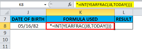
It returns the output value i.e. 36 years.
Example #4
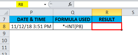
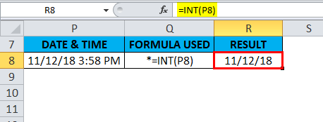
Usually, Excel stores the date value as a number, where it considers the date as an integer and the time as a decimal portion. If a cell contains a date and time as a combined value, you can extract date value only by using the INT function in Excel. Here cell “P8” contains date and time as a combined value. Here I need to specifically extract the date value in cell “R8.”
Select the cell R8 where the INT function needs to be applied.
Click the insert function button (fx) under the formula toolbar; a dialog box will appear, type the keyword “INT” in the search for a function box; INT function will appear in select a function box. Double click on the INT function.
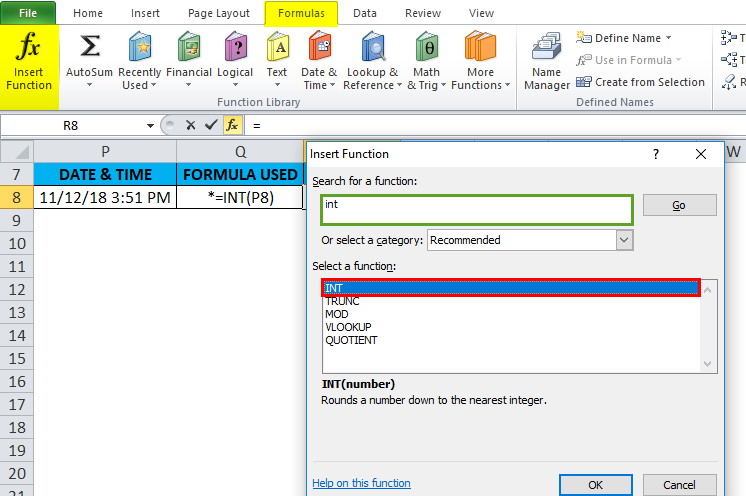
A dialog box appears where arguments (number) for the INT function need to be filled or entered.
i.e. =INT(P8)
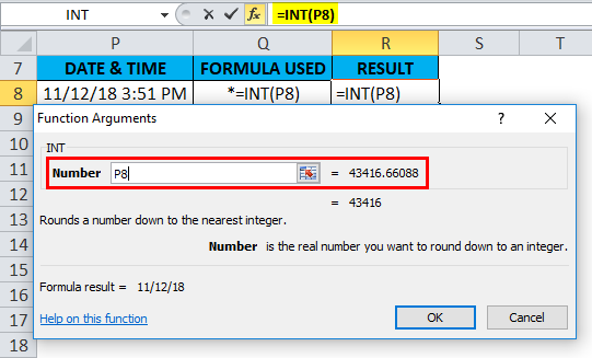
It removes a decimal portion from the date & time value and returns only the date portion as a number, where we need to discard the fraction value by formatting in output value.
i.e. 11/12/18
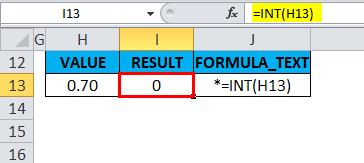
Example #5
The below-mentioned table contains a value less than 1 in cell “H13”, i.e. 0.70, which is a positive number; I need to find out the nearest integer for decimal value, i.e. 0.70, using the INT function in Excel. Select the cell I13 where the INT function needs to be applied.
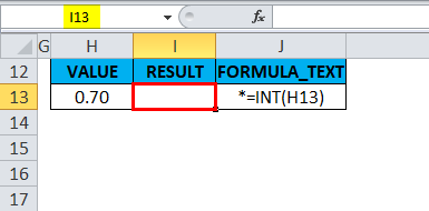
Click the insert function button (fx) under the formula toolbar; a dialog box will appear, type the keyword “INT” in the search for a function box, INT function will appear in select a function box. Double click on the INT function.
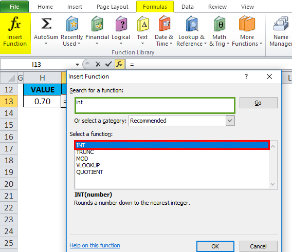
A dialog box appears where arguments (number) for the INT function need to be filled or entered.
i.e. =INT(H13)
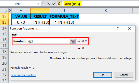
Here, it removes decimal from the number and returns the integer part of the number, i.e. 0
Things to Remember
- In INT function, Positive numbers are rounded toward 0 while negative numbers are rounded away from 0. E.G. =INT(2.5) returns 2 and =INT(-2.5) returns -3.
- Both INT() and TRUNC() functions are similar when applied to positive numbers; both of them can be used to convert a value to its integer portion.
- If any wrong type of argument is entered in the syntax of the function, it results in #VALUE! error.
- If the referred cell is not a valid or invalid reference in INT function, it will return or results in #REF! error.
- #NAME? error occurs when Excel does not recognize specific text in the formula of INT function.
Recommended Articles
This has been a guide to INT Function in Excel. Here we discuss the INT Formula in Excel and how to use the INT function in Excel along with practical examples and downloadable excel templates. You can also go through our other suggested articles –
- MID Function in Excel
- EVEN Excel Function
- POWER Function in Excel
- Excel Formula For Rank
The INT function is one of the math functions of Excel.
It Rounds a number down to a Nearest integer.
We can find this function in Math & trig of insert function Tab.
How to use INT function in excel
- Click on an empty cell (like F5 )
2. Click on the fx icon (or press shift+F3)
3. In the insert function tab you will see all functions
4. Select math and trig category
5. Select INT function
6. Then select ok
7. In the function Arguments Tab you will see the INT function
8. In the number section you can enter the value to round (for example 1.5)
9. If you enter +1.5 result will be 1
10. If you enter 2.5 result will be 2
11. If you enter -1.5 result will be -2
12. If you enter -2.5 result will be -3
13. You will see results in the formula result section
Examples of INT function in excel
Example 1:
How to use INT function in excel
You can see examples of INT function below:
int(2.4) ----->>>>answer is  2

int(1.4) ----->>>>answer is  1

int(0) ----->>>>answer is    0

int(-1.6) ----->>>>answer is  -2

int(-2.6) ----->>>>answer is  -3
What is the purpose of INT function?
It Rounds a number down to a Nearest integer.
What is the Return value of INT function?
It returns a number.
How many arguments does INT function have?
This function has just 1 Argument.
The argument of INT function is number.
In the number section you can enter the value to round (for example 1.5).
The argument of INT function is required and not optional.
INT(number) = number
Which version of excel supports INT function?
This function is available for all excel versions (2003-2019)
Errors in INT function
INT related functions :
- TRUNC Function
- ROUND Function
- ROUNDDOWN Function
- ROUNDUP Function
- MROUND Function
- FLOOR function
- CEILING function
I’m an Excel Expert with 10+ of experience, specializing in Excel Worksheets, Advanced Charting, Functions, data visualization, pivot tables, and data analytics. I help businesses to manage projects and analyze data with the use of Excel.
Login

This Excel tutorial explains how to use the Excel INT function with syntax and examples.
Description
The Microsoft Excel INT function returns the integer portion of a number.
The INT function is a built-in function in Excel that is categorized as a Math/Trig Function. It can be used as a worksheet function (WS) and a VBA function (VBA) in Excel. As a worksheet function, the INT function can be entered as part of a formula in a cell of a worksheet. As a VBA function, you can use this function in macro code that is entered through the Microsoft Visual Basic Editor.
Syntax
The syntax for the INT function in Microsoft Excel is:
INT( expression )
Parameters or Arguments
- expression
- A numeric expression whose integer portion is returned.
Note
- If the expression is negative, the INT function will return the first negative number that is less than or equal to the expression.
Returns
The INT function returns an integer value.
Applies To
- Excel for Office 365, Excel 2019, Excel 2016, Excel 2013, Excel 2011 for Mac, Excel 2010, Excel 2007, Excel 2003, Excel XP, Excel 2000
Type of Function
- Worksheet function (WS)
- VBA function (VBA)
Example (as Worksheet Function)
Let’s look at some Excel INT function examples and explore how to use the INT function as a worksheet function in Microsoft Excel:
Based on the Excel spreadsheet above, the following INT examples would return:
=INT(A1)
Result: 210

=INT(A2)
Result: 2

=INT(A3)
Result: -3

=INT(-4.5)
Result: -5
Example (as VBA Function)
The INT function can also be used in VBA code in Microsoft Excel.
Let’s look at some Excel INT function examples and explore how to use the INT function in Excel VBA code:
Dim LNumber As Double

LNumber = Int(210.67)
In this example, the variable called LNumber would now contain the value of 210.