
Excel for Microsoft 365 Excel for Microsoft 365 for Mac Excel for the web Excel 2021 Excel 2021 for Mac Excel 2019 Excel 2019 for Mac Excel 2016 Excel 2016 for Mac Excel 2013 Excel 2010 Excel 2007 Excel for Mac 2011 Excel Starter 2010 More…Less
This article describes the formula syntax and usage of the INDIRECT function in Microsoft Excel.
Description
Returns the reference specified by a text string. References are immediately evaluated to display their contents. Use INDIRECT when you want to change the reference to a cell within a formula without changing the formula itself.
Syntax
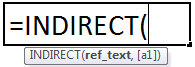
INDIRECT(ref_text, [a1])
The INDIRECT function syntax has the following arguments:
-
Ref_text Required. A reference to a cell that contains an A1-style reference, an R1C1-style reference, a name defined as a reference, or a reference to a cell as a text string. If ref_text is not a valid cell reference, INDIRECT returns the #REF! error value.
-
If ref_text refers to another workbook (an external reference), the other workbook must be open. If the source workbook is not open, INDIRECT returns the #REF! error value.
Note External references are not supported in Excel Web App.
-
If ref_text refers to a cell range outside the row limit of 1,048,576 or the column limit of 16,384 (XFD), INDIRECT returns a #REF! error.
Note This behavior is different from Excel versions earlier than Microsoft Office Excel 2007, which ignore the exceeded limit and return a value.
-
-
A1 Optional. A logical value that specifies what type of reference is contained in the cell ref_text.
-
If a1 is TRUE or omitted, ref_text is interpreted as an A1-style reference.
-
If a1 is FALSE, ref_text is interpreted as an R1C1-style reference.
-
Example
Copy the example data in the following table, and paste it in cell A1 of a new Excel worksheet. For formulas to show results, select them, press F2, and then press Enter. If you need to, you can adjust the column widths to see all the data.
|
Data |
||
|
B2 |
1.333 |
|
|
B3 |
45 |
|
|
George |
10 |
|
|
5 |
62 |
|
|
Formula |
Description |
Result |
|
‘=INDIRECT(A2) |
Value of the reference in cell A2. The reference is to cell B2, which contains the value 1.333. |
1.333 |
|
‘=INDIRECT(A3) |
Value of the reference in cell A3. The reference is to cell B3, which contains the value 45. |
45 |
|
‘=INDIRECT(A4) |
Because cell B4 has the defined name «George,» the reference to that defined name is to cell B4, which contains the value 10. |
10 |
|
‘=INDIRECT(«B»&A5) |
Combines «B» with the value in A5, which is 5. This, in turn, refers to cell B5, which contains the value 62. |
62 |
Need more help?
Want more options?
Explore subscription benefits, browse training courses, learn how to secure your device, and more.
Communities help you ask and answer questions, give feedback, and hear from experts with rich knowledge.
Returns a reference to a range
What is the Excel INDIRECT Function?
The Excel INDIRECT Function[1] returns a reference to a range. The INDIRECT function does not evaluate logical tests or conditions. Also, it will not perform calculations. Basically, this function helps lock the specified cell in a formula. Due to this, we can change a cell reference within a formula without changing the formula itself.
One advantage of this function is that the indirect references won’t change even when new rows or columns are inserted in the worksheet. Similarly, references won’t change when we delete existing ones.
Formula
=INDIRECT(ref_text, [a1])
Where:
ref_text is the reference supplied as text
a1 is the logical value
The type of reference, contained in the ref_text argument, is specified by a1.
When a1 is TRUE or is omitted, then ref_text is interpreted as an A1-style cell reference.
When a1 is FALSE, then ref_text is treated as an R1C1 reference.
A1 style is the usual reference type in Excel. It is preferable to use A1 references. In this style, a column is followed by a row number.
R1C1 style is completely opposite of A1 style. Here, rows are followed by columns. For example, R2C1 refers to cell A2 which is in row 2, column 1 in a sheet. If there is no number after the letter, then it means we are referring to the same row or column.
To learn more, launch our free Excel crash course now!
Example of Excel INDIRECT in action
Let’s understand the formula through an example. Suppose A1 = 32 and using the INDIRECT function, we give reference A1 as shown below:
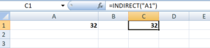
In the above example, the INDIRECT function converted a text string into a cell reference. The INDIRECT function helps us put the address of one cell (A1 in our example) into another as a usual text string, and then get the value of the first cell by acknowledging the second.
How is the INDIRECT function useful to Excel users?
Yes, it is indeed a useful function. Let’s take a few examples to understand the merits of the INDIRECT function.
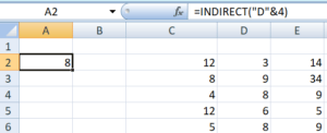
For an array of numbers:
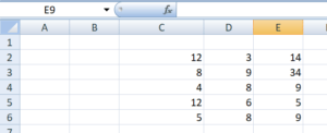
When I give the formula Indirect(“D”&4), I will get 8. This is so as it will refer to D4.
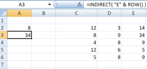
When I use the formula INDIRECT(“E” & ROW() ), I used the EXCEL ROW function to return the reference to the current row number (i.e., 3), and used this to form part of the cell reference. Therefore, the Indirect formula returns the value from cell E3.
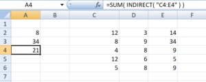
When I use the formula SUM( INDIRECT( “C4:E4” ) ), the Indirect function returns a reference to the range C4:E4, and then passes this to Excel’s SUM function. The SUM function, therefore, returns the sum of cells C4, D4, and E4, that is (4 + 8 + 9).
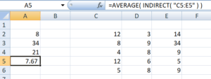
Similarly, when I use the formula AVERAGE ( INDIRECT( “C5:E5” ) ), the INDIRECT function returns a reference to the range C5:E5, and then passes this to Excel’s AVERAGE function.
The usefulness of Excel’s INDIRECT function is not just limited to building “dynamic” cell references. In addition, it can also be used to refer to cells in other worksheets.
To learn more, launch our free Excel crash course now!
How to lock a cell reference using INDIRECT function
Generally, when we add or delete rows or columns in Excel, the cell references change automatically. If you wish to prevent this from happening, the INDIRECT function is quite useful.
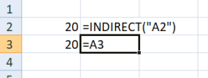
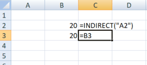
In the screenshot below, I used the INDIRECT function for A2 and gave a plain reference for A3.
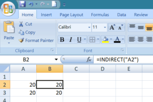
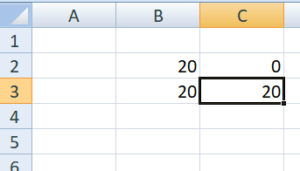
When I insert a new column, what will happen? The cell equal to the logical operator still returns 20, as its formula was automatically changed to =B3.
However, the cell with the INDIRECT formula now returns 0, because the formula was not changed when a new row was inserted and it still refers to cell A1, which is currently empty:
So the Excel INDIRECT function would be useful in a scenario when we don’t want the formula to get changed automatically.
Free Excel Course
To keep learning about Excel functions and developing your skills, check out our Free Excel Crash Course! Learn how to create more sophisticated financial analysis and modeling to become a successful financial analyst.
Additional Resources
Thanks for reading CFI’s guide to the important Excel INDIRECT function! By taking the time to learn and master these functions, you’ll significantly speed up your financial analysis. To learn more, check out these additional CFI resources:
- Excel Functions for Finance
- Advanced Excel Formulas Course
- Advanced Excel Formulas You Must Know
- Excel Shortcuts for PC and Mac
- See all Excel resources
The INDIRECT function returns a valid cell reference from a given text string. INDIRECT is useful when you need to build a text value by concatenating separate text strings that can then be interpreted as a valid cell reference.
INDIRECT is a volatile function, and can cause performance issues in large or complex worksheets.
INDIRECT takes two arguments, ref_text and a1. Ref_text is the text string to evaluate as a reference. A1 indicates the reference style for the incoming text value. When a1 is TRUE (the default value), the style is «A1». When a1 is FALSE, the style is «R1C1». For example:
=INDIRECT("A1") // returns reference like =A1
=INDIRECT("R1C1",FALSE) // returns reference like =R1C1
The purpose of INDIRECT may at first seem baffling (i.e. Why use text when you can just provide a proper reference?) but there are many situations where the ability to create a reference from text is useful, including:
- A formula that needs a variable sheet name
- A formula that can assemble a cell reference from bits of text
- A fixed reference that will not change even when rows or columns are deleted
- Creating numeric arrays with the ROW function in complex formulas
Note: INDIRECT is a volatile function and can cause performance problems in large or complex worksheets. Use with care.
Example #1 — Variable worksheet name
In the example shown above, INDIRECT is set up to use a variable sheet name like this:
=INDIRECT(B5&"!A1") // sheet name in B5 is variable
The formula in B5, copied down, concatenates the text in B5 to the string «!A1» and returns the result to INDIRECT. The INDIRECT function then evaluates the text and converts it into a proper reference. The results in C5:C9 are the values from cell A1 in 5 sheets listed in column B.
The formula is dynamic in that responds to the values in column B. In other words, if a different sheet name is entered in column B5, the value from cell A1 in the new sheet is returned. With the same approach, you could allow a user to select a sheet name with a dropdown list, then construct a reference to the selected sheet with INDIRECT.
Note: sheet names that contain punctuation or space must be enclosed in single quotes (‘), as explained in this example. This is not specific to the INDIRECT function; the same limitation is true in all formulas.
Example #2 — variable lookup table
In the worksheet below, VLOOKUP is used to get costs for two vendors, A and B. Using the vendor indicated in column F, VLOOKUP automatically uses the correct table:

The formula in G5 is:
=VLOOKUP(E5,INDIRECT("vendor_"&F5),2,0)
Read the full explanation here.
Example #3 — Fixed reference
The reference created by INDIRECT will not change even when cells, rows, or columns are inserted or deleted. For example, the formula below will always refer to the first 100 rows of column A, even if rows in that range are deleted or inserted:
=INDIRECT("A1:A100") // will not change
Example #4 — named range
The INDIRECT function can easily be used with named ranges. In the worksheet below, there are two named ranges: Group1 (B5:B12) and Group2 (C5:C12). When «Group1» or «Group2» is entered in cell F5, the formula in cell F6 sums the appropriate range using INDIRECT like this:
=SUM(INDIRECT(F5))
The value in F5 is text, but INDIRECT converts the text into a valid range.

A specific example of this approach is using named ranges to make dependent dropdown lists.
Example #5 — Generate numeric array
A more advanced use of INDIRECT is to create a numeric array with the ROW function like this:
ROW(INDIRECT("1:10")) // create {1;2;3;4;5;6;7;8;9;10}
One use case is explained in this formula, which sums the bottom n values in a range. You may also run into ROW + INDIRECT idea in more complex formulas that need to assemble a numeric array «on-the-fly». One example is this formula, designed to strip numeric characters from a string.
Notes
- References created by INDIRECT are evaluated in real time and the content of the reference is displayed.
- When ref_text is an external reference to another workbook, the workbook must be open.
- a1 is optional. When omitted, a1 is TRUE = A1 style reference.
- When a1 is set to FALSE, INDIRECT will create an R1C1-style reference.
- INDIRECT is a volatile function, and can cause performance issues in large or complex worksheets.
Using Excel INDIRECT function to lock a cell reference
- Enter any value in any cell, say, number 20 in cell A1.
- Refer to A1 from two other cells in different ways: =A1 and =INDIRECT(“A1”)
- Insert a new row above row 1.
Contents
- 1 How do you find the indirect formula in Excel?
- 2 How do you use indirect on another sheet?
- 3 How do I pull data from another sheet in Excel based on cell value?
- 4 How do you write an indirect formula?
- 5 What is an example of indirect?
- 6 What is indirect function in Excel with example?
- 7 How do you use text function in Excel?
- 8 How do you use cell values in Excel?
- 9 Can Excel pull data from another sheet?
- 10 How do I pull data from another sheet in sheets?
- 11 What are the 3 types of cell references in Excel?
- 12 How do I reference another sheet in Excel?
- 13 How do I make column letters in Excel?
- 14 What is indirect Excel?
- 15 How do you use indirect object in a sentence?
- 16 What is an indirect object pronoun?
- 17 Can you use indirect with Vlookup?
- 18 How is indirect function used in data validation?
- 19 How do I write text in Excel?
- 20 How do I write formulas in Excel?
How do you find the indirect formula in Excel?
To show the cell formulas, instead of values, revise the formula, to wrap it with the FORMULATEXT function.
- In cell C5, revise the formula: =FORMULATEXT(INDIRECT(“‘” & $B5 & “‘!” & C$4))
- Press Enter, to see the result.
How do you use indirect on another sheet?
Let`s say you want to calculate the SUM result of some values of a worksheet by referring it to another worksheet. To do this, make a new worksheet named S4. In cell A2, write down S1. Type the formula, =SUM(INDIRECT(“'”&A2&”'!”&”A1:A4”)) in cell B2 and you will get the result 10 in cell B2.
How do I pull data from another sheet in Excel based on cell value?
To pull values from another worksheet, we need to follow these steps:
- Select cell C3 and click on it.
- Insert the formula: =VLOOKUP(B3,'Sheet 2'!$ B$3:$C$7,2,0)
- Press enter.
- Drag the formula down to the other cells in the column by clicking and dragging the little “+” icon at the bottom-right of the cell.
How do you write an indirect formula?
Cell Reference
For example, take a look at the INDIRECT function below. Explanation: =INDIRECT(A1) reduces to =INDIRECT("D1"). The INDIRECT function converts the text string "D1" into a valid cell reference. In other words, =INDIRECT("D1") reduces to =D1.
What is an example of indirect?
The definition of indirect is a person or thing that is not straight, or not direct and honest. An example of indirect is a flight that goes from Los Angeles to Denver in order to get to Seattle; an indirect flight.
What is indirect function in Excel with example?
The INDIRECT function is useful when you want to return a value, based on a text string. For example, select a range name from a drop down list, and get the total amount for the selected range. In this screen shot, choose Actual or Budget in cell B2, and the total appears in cell B3.
How do you use text function in Excel?
The Excel TEXT Function is used to convert numbers to text within a spreadsheet. Essentially, the function will convert a numeric value into a text string. TEXT is available in all versions of Excel.
Tips.
| + | Plus sign |
|---|---|
| / | Forward slash |
| ! | Exclamation mark |
| <> | Less than and greater than |
How do you use cell values in Excel?
Use cell references in a formula
- Click the cell in which you want to enter the formula.
- In the formula bar. , type = (equal sign).
- Do one of the following, select the cell that contains the value you want or type its cell reference.
- Press Enter.
Can Excel pull data from another sheet?
To pull data from one excel sheet to another is the process of taking the data to be it in a column or a row to another excel sheet. Once we pull values from another sheet, which is commonly done, we can save on time taken which we would otherwise keep in inserting the values in columns or the rows.
How do I pull data from another sheet in sheets?
Import data from another spreadsheet
- In Sheets, open a spreadsheet.
- In an empty cell, enter =IMPORTRANGE.
- In parenthesis, add the following specifications in quotation marks and separated by a comma*: The URL of the spreadsheet in Sheets.
- Press Enter.
- Click Allow access to connect the 2 spreadsheets.
What are the 3 types of cell references in Excel?
Relative, Absolute and Mixed
A key element of a formula is the cell reference, and there are three types: Relative. Absolute. Mixed.
How do I reference another sheet in Excel?
To reference a cell or range of cells in another worksheet in the same workbook, put the worksheet name followed by an exclamation mark (!) before the cell address. For example, to refer to cell A1 in Sheet2, you type Sheet2!A1. For example, to refer to cells A1:A10 in Sheet2, you type Sheet2!A1:A10.
How do I make column letters in Excel?
To convert a column number to an Excel column letter (e.g. A, B, C, etc.) you can use a formula based on the ADDRESS and SUBSTITUTE functions. With this information, ADDRESS returns the text "A1".
What is indirect Excel?
The Excel INDIRECT Function returns a reference to a range. The INDIRECT function does not evaluate logical tests or conditions.Basically, this function helps lock the specified cell in a formula. Due to this, we can change a cell reference within a formula without changing the formula itself.
How do you use indirect object in a sentence?
An indirect object is an optional part of a sentence; it's the recipient of an action. In the sentence “Jake gave me some cereal,” the word “me” is the indirect object; I'm the person who got cereal from Jake.
What is an indirect object pronoun?
An indirect object pronoun is used instead of a noun to show the person or thing an action is intended to benefit or harm, for example, me in He gave me a book.; Can you get me a towel?; He wrote to me.
Can you use indirect with Vlookup?
INDIRECT & VLOOKUP
You may need to perform a VLOOKUP on multiple ranges at once, dependent on certain cell values. For these instances, the INDIRECT Function can be used to define a lookup range, or even create a dynamic reference to multiple sheets.
How is indirect function used in data validation?
Data Validation has been applied to the cells in column A with the formula =INDIRECT($A$1) note that this is an Absolute reference, so it will always be referring to cell A1 In other words, cells in this column will be the list which is the same as the text that is held in A1 - Region.
How do I write text in Excel?
Combine Cells With Text and a Number
- Select the cell in which you want the combined data.
- Type the formula, with text inside double quotes. For example: ="Due in " & A3 & " days" NOTE: To separate the text strings from the numbers, end or begin the text string with a space.
- Press Enter to complete the formula.
How do I write formulas in Excel?
Create a simple formula in Excel
- On the worksheet, click the cell in which you want to enter the formula.
- Type the = (equal sign) followed by the constants and operators (up to 8192 characters) that you want to use in the calculation. For our example, type =1+1. Notes:
- Press Enter (Windows) or Return (Mac).
Excel formulae allow users to perform basic calculations such as addition, subtraction, or multiplication, as well as find out the average or percentage of a cell range. Not only is it possible to apply these formulae to numeric values, but they also function with other data types, such as text, date, or time.
The Excel INDIRECT function allows you to lock a reference to a single cell, a cell range, or a cell from another sheet. This means that the references won’t change even if you edit the rows or columns in your spreadsheet — either by adding new ones or deleting existing ones. This is because the INDIRECT function converts a text string into a valid reference. You avoid returning values from a broken formula or simply #REF! errors.
In this article, you’ll learn what the INDIRECT function in Excel is, the INDIRECT formula syntax, and how to lock a cell reference to effectively manage formulae and level up your spreadsheet skills.
What is the Excel INDIRECT function?
The Excel INDIRECT function works like any other formula in your spreadsheet. Unlike the majority of formulae, this function is aimed at converting a text string into a valid reference. Moreover, the “&” operator can be included in the formula to create text strings. Let’s take a look at the INDIRECT syntax to understand how it works.
INDIRECT Formula Syntax
Below is the syntax for the INDIRECT formula and the meaning behind each parameter.
=INDIRECT (ref_text, [a1])
- ref_text is the cell reference provided in text format, so it should be enclosed in speech marks. For example, to reference cell A1, write “A1”.
- [a1] is a logical value that describes the reference style used in Excel. The A1 reference style follows the usual sequence of column (A) and row (1); the R1C1 reference style follows the opposite sequence, row (R1) and column (C1). When [a1] is set to TRUE or left empty, the ref_text is read as an A1 reference style; if set to FALSE, then it will be read as R1C1.
Now that you know what the Excel INDIRECT function is and its formula syntax, let’s see how it can be applied to various examples.
How to use the INDIRECT function in Excel?
We can use the Excel INDIRECT function to lock a specified cell in a formula; this allows you to change the cell reference within a formula without affecting it. Whether you add or delete rows or columns, it does not affect indirect references.
How to lock a cell reference using the INDIRECT function in Excel?
Let’s start by using the INDIRECT formula for simple conversion from text to a valid cell reference.
- 1. Open your spreadsheet and enter a numeric value in any cell. Here, I will type in “56” in cell A1.

Excel INDIRECT Function — Enter numeric value
- 2. Enter the INDIRECT formula in any cell you wish. Remember that, as soon as you start typing, Excel will prompt you with the full formula. Here, I will enter the formula in cell B1 and refer to cell A1 to pull the numeric value: “INDIRECT(“A1”).

Excel INDIRECT Function — Enter INDIRECT Formula
- 3. Your spreadsheet should now show the same values in both cells.

Excel INDIRECT Function — Returns cell values
As you can see, the INDIRECT function converts a text string (here, “A1”) into a valid cell reference to return the value of the referenced cell. Let’s explore further basic examples using the INDIRECT function in Excel for an array of numbers using the “&” operator.
How to Reference Another Sheet or Workbook in Excel?
Sometimes you have to reference or merge data from multiple sheets or spreadsheets. Here’s how to reference another sheet or workbook in Excel.
READ MORE

How to use the “&” operator with the INDIRECT function in Excel?
The “&” is the CONCATENATE operator in Excel. It’s helpful when you want to join the results of two text strings. It’s normally used in conjunction with other functions such as SUM, but you can also use it for a single cell reference, as shown below.
- 1. Go to your spreadsheet and type in the INDIRECT formula as before, and include the “&” operator between the column and the row reference. Here, we have used “=INDIRECT(“E”&3)” to return the value from cell E3, which is “5”.

Excel INDIRECT Function — Use & operator
- 2. Try to add or delete a column to check how the formula behaves. Here, we will insert a column between D and E.

Excel INDIRECT Function — Add or delete column
- 3. As you can see, instead of returning an error message, Excel still returns a valid reference. Here, the valid reference is “0”, as the cells are empty.

Excel INDIRECT Function — Valid reference to empty cell
Let’s see what happens if I combine the ROW function with the INDIRECT function in Excel.
How to use the ROW function with the INDIRECT function in Excel?
Using the “&” operator, you can combine the ROW and INDIRECT functions to return a reference based on the row where you enter the formula. In this example, I want to return the cell reference from the row where I add my formula — Row 1.
- 1. Type =INDIRECT(“ref_text”&ROW()) in any of the available cells, only specifying the ref_text parameter.
- 2. Here, we will reference column D and enter the formula in row 1.

Excel INDIRECT Function — ROW function
As you have seen, the formula now returns the value based on the formula’s row number; here, the numeric value is “4”, corresponding to cell D1.
How to use the SUM function with the INDIRECT function in Excel?
The SUM function is used to add numeric values together. When combined with the INDIRECT function, it will return the sum of referenced cells.
- 1. Type in the formula =SUM(INDIRECT(“ref_text”)) in the cell you wish to return your SUM. While the INDIRECT function returns the referenced cells, the SUM function will be in charge of returning the sum.
- 2. Here, we will use =SUM(INDIRECT(«D1:D5»)) to return the sum of the cell range, including all numeric values in column D.

Excel INDIRECT Function — SUM function
As you can see, the formula returns the sum of all numbers by referring to the cell range. Here, the valid reference is “39”, and the text value used to refer is “D1:D5”.
If I delete row 4 completely, the INDIRECT function acknowledges this change in the cell range reference and will return a new total.

Excel INDIRECT Function — New value for SUM function
How to use the AVERAGE function with the INDIRECT function in Excel?
Similarly, when we combine the AVERAGE and INDIRECT functions, it first refers to the cell range and then performs the calculation, in this case, the average.
- 1. Type in the formula =AVERAGE(INDIRECT(“ref_text”)) in any cell.
- 2. Here, we will use =AVERAGE(INDIRECT(«D1:D5»)) to return the average of the cell range used in the previous example.

Excel INDIRECT Function — AVERAGE function
If I add a new row, the values within the data range change. The INDIRECT function will recognize this, and so the data range will no longer include the value “15”. Instead, it returns the average of the first 5 rows (as specified in the formula). Here, it returns a new value of “5.4”.

Excel INDIRECT Function — New value for AVERAGE function
The usefulness of Excel’s INDIRECT function is not just limited to locking a cell reference for the correct functioning of formulae. We will now see how it can be used to refer to a cell in another sheet.
How to reference another sheet using the INDIRECT function in Excel?
Let’s see how the INDIRECT function can return cell values from another sheet.
- 1. Open a new sheet where you will use the formula. To refer to a cell in another sheet, we will include the sheet name and the cell in the “ref_text” parameter.
- 2. It’s important to include it between speech marks and add an exclamation after the sheet name. For example, =INDIRECT(«JANUARY!A1»).

Excel INDIRECT Function — Reference another sheet cell
As you can see, it has returned the same value in the referenced cell from another sheet. The formula will behave in the same way regardless of the number of sheets or information held in your spreadsheets.
Want to Boost Your Team’s Productivity and Efficiency?
Transform the way your team collaborates with Confluence, a remote-friendly workspace designed to bring knowledge and collaboration together. Say goodbye to scattered information and disjointed communication, and embrace a platform that empowers your team to accomplish more, together.
Key Features and Benefits:
- Centralized Knowledge: Access your team’s collective wisdom with ease.
- Collaborative Workspace: Foster engagement with flexible project tools.
- Seamless Communication: Connect your entire organization effortlessly.
- Preserve Ideas: Capture insights without losing them in chats or notifications.
- Comprehensive Platform: Manage all content in one organized location.
- Open Teamwork: Empower employees to contribute, share, and grow.
- Superior Integrations: Sync with tools like Slack, Jira, Trello, and more.
Limited-Time Offer: Sign up for Confluence today and claim your forever-free plan, revolutionizing your team’s collaboration experience.
Conclusion
As you can see, the Excel INDIRECT function is essential for users who want to perform more complex tasks on their spreadsheets. By locking references to cells, you can return valid results from different formulae, regardless of whether you change the rows or columns within your spreadsheet. Overall, you have more control over your dynamic data whilst avoiding the time-consuming alternative of copying and pasting values across your spreadsheet.
This guide has shown you what the INDIRECT function is and its syntax. By the end of this article, you should know how to use the INDIRECT function to lock a reference to a cell, how to lock a reference to a cell range combined with another formula, and how to reference a cell from another sheet.
If you would like to know more about referencing, read our article on How to Reference Another Sheet or Workbook in Excel. If you prefer using Google Sheets, then you’ll find Linking Google Sheets: How To Reference Another Sheet of great help.
Содержание
- INDIRECT function
- Description
- Syntax
- Example
- INDIRECT Function
- Summary
- Purpose
- Return value
- Arguments
- Syntax
- Usage notes
- Example #1 — Variable worksheet name
- Example #2 — variable lookup table
- Example #3 — Fixed reference
- Example #4 — named range
- Example #5 — Generate numeric array
- How To Use Indirect In Excel?
- How do you find the indirect formula in Excel?
- How do you use indirect on another sheet?
- How do I pull data from another sheet in Excel based on cell value?
- How do you write an indirect formula?
- What is an example of indirect?
- What is indirect function in Excel with example?
- How do you use text function in Excel?
- How do you use cell values in Excel?
- Can Excel pull data from another sheet?
- How do I pull data from another sheet in sheets?
- What are the 3 types of cell references in Excel?
- How do I reference another sheet in Excel?
- How do I make column letters in Excel?
- What is indirect Excel?
- How do you use indirect object in a sentence?
- What is an indirect object pronoun?
- Can you use indirect with Vlookup?
- How is indirect function used in data validation?
- How do I write text in Excel?
- How do I write formulas in Excel?
- Excel INDIRECT Function
- What is the Excel INDIRECT Function?
- Formula
- Example of Excel INDIRECT in action
- How is the INDIRECT function useful to Excel users?
- How to lock a cell reference using INDIRECT function
- Free Excel Course
- Additional Resources
INDIRECT function
This article describes the formula syntax and usage of the INDIRECT function in Microsoft Excel.
Description
Returns the reference specified by a text string. References are immediately evaluated to display their contents. Use INDIRECT when you want to change the reference to a cell within a formula without changing the formula itself.
Syntax
The INDIRECT function syntax has the following arguments:
Ref_text Required. A reference to a cell that contains an A1-style reference, an R1C1-style reference, a name defined as a reference, or a reference to a cell as a text string. If ref_text is not a valid cell reference, INDIRECT returns the #REF! error value.
If ref_text refers to another workbook (an external reference), the other workbook must be open. If the source workbook is not open, INDIRECT returns the #REF! error value.
Note External references are not supported in Excel Web App.
If ref_text refers to a cell range outside the row limit of 1,048,576 or the column limit of 16,384 (XFD), INDIRECT returns a #REF! error.
Note This behavior is different from Excel versions earlier than Microsoft Office Excel 2007, which ignore the exceeded limit and return a value.
A1 Optional. A logical value that specifies what type of reference is contained in the cell ref_text.
If a1 is TRUE or omitted, ref_text is interpreted as an A1-style reference.
If a1 is FALSE, ref_text is interpreted as an R1C1-style reference.
Example
Copy the example data in the following table, and paste it in cell A1 of a new Excel worksheet. For formulas to show results, select them, press F2, and then press Enter. If you need to, you can adjust the column widths to see all the data.
Источник
INDIRECT Function

Summary
The Excel INDIRECT function returns a valid cell reference from a given text string. INDIRECT is useful when you want to assemble a text value that can be used as a valid reference.
Purpose
Return value
Arguments
- ref_text — A reference supplied as text.
- a1 — [optional] A boolean to indicate A1 or R1C1-style reference. Default is TRUE = A1 style.
Syntax
Usage notes
The INDIRECT function returns a valid cell reference from a given text string. INDIRECT is useful when you need to build a text value by concatenating separate text strings that can then be interpreted as a valid cell reference.
INDIRECT takes two arguments, ref_text and a1. Ref_text is the text string to evaluate as a reference. A1 indicates the reference style for the incoming text value. When a1 is TRUE (the default value), the style is «A1». When a1 is FALSE, the style is «R1C1». For example:
The purpose of INDIRECT may at first seem baffling (i.e. Why use text when you can just provide a proper reference?) but there are many situations where the ability to create a reference from text is useful, including:
- A formula that needs a variable sheet name
- A formula that can assemble a cell reference from bits of text
- A fixed reference that will not change even when rows or columns are deleted
- Creating numeric arrays with the ROW function in complex formulas
Note: INDIRECT is a volatile function and can cause performance problems in large or complex worksheets. Use with care.
Example #1 — Variable worksheet name
In the example shown above, INDIRECT is set up to use a variable sheet name like this:
The formula in B5, copied down, concatenates the text in B5 to the string «!A1» and returns the result to INDIRECT. The INDIRECT function then evaluates the text and converts it into a proper reference. The results in C5:C9 are the values from cell A1 in 5 sheets listed in column B.
The formula is dynamic in that responds to the values in column B. In other words, if a different sheet name is entered in column B5, the value from cell A1 in the new sheet is returned. With the same approach, you could allow a user to select a sheet name with a dropdown list, then construct a reference to the selected sheet with INDIRECT.
Note: sheet names that contain punctuation or space must be enclosed in single quotes (‘), as explained in this example. This is not specific to the INDIRECT function; the same limitation is true in all formulas.
Example #2 — variable lookup table
In the worksheet below, VLOOKUP is used to get costs for two vendors, A and B. Using the vendor indicated in column F, VLOOKUP automatically uses the correct table:
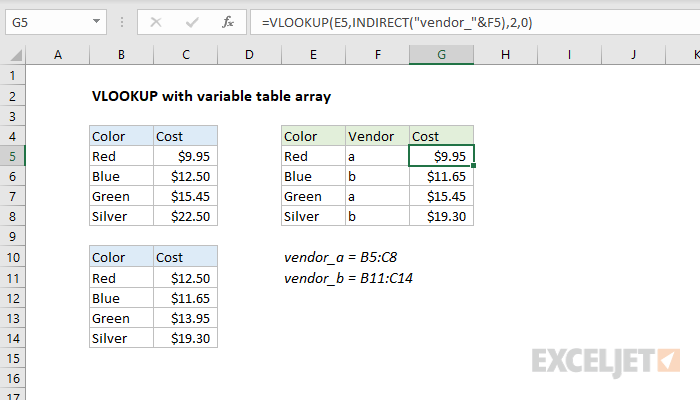
The formula in G5 is:
Example #3 — Fixed reference
The reference created by INDIRECT will not change even when cells, rows, or columns are inserted or deleted. For example, the formula below will always refer to the first 100 rows of column A, even if rows in that range are deleted or inserted:
Example #4 — named range
The INDIRECT function can easily be used with named ranges. In the worksheet below, there are two named ranges: Group1 (B5:B12) and Group2 (C5:C12). When «Group1» or «Group2» is entered in cell F5, the formula in cell F6 sums the appropriate range using INDIRECT like this:
The value in F5 is text, but INDIRECT converts the text into a valid range.
Example #5 — Generate numeric array
A more advanced use of INDIRECT is to create a numeric array with the ROW function like this:
One use case is explained in this formula, which sums the bottom n values in a range. You may also run into ROW + INDIRECT idea in more complex formulas that need to assemble a numeric array «on-the-fly». One example is this formula, designed to strip numeric characters from a string.
Источник
How To Use Indirect In Excel?
Using Excel INDIRECT function to lock a cell reference
- Enter any value in any cell, say, number 20 in cell A1.
- Refer to A1 from two other cells in different ways: =A1 and =INDIRECT(“A1”)
- Insert a new row above row 1.
How do you find the indirect formula in Excel?
To show the cell formulas, instead of values, revise the formula, to wrap it with the FORMULATEXT function.
- In cell C5, revise the formula: =FORMULATEXT(INDIRECT(“‘” & $B5 & “‘!” & C$4))
- Press Enter, to see the result.
How do you use indirect on another sheet?
Let`s say you want to calculate the SUM result of some values of a worksheet by referring it to another worksheet. To do this, make a new worksheet named S4. In cell A2, write down S1. Type the formula, =SUM(INDIRECT(“’”&A2&”’!”&”A1:A4”)) in cell B2 and you will get the result 10 in cell B2.
How do I pull data from another sheet in Excel based on cell value?
To pull values from another worksheet, we need to follow these steps:
- Select cell C3 and click on it.
- Insert the formula: =VLOOKUP(B3,’Sheet 2′!$ B$3:$C$7,2,0)
- Press enter.
- Drag the formula down to the other cells in the column by clicking and dragging the little “+” icon at the bottom-right of the cell.
How do you write an indirect formula?
Cell Reference
For example, take a look at the INDIRECT function below. Explanation: =INDIRECT(A1) reduces to =INDIRECT(«D1»). The INDIRECT function converts the text string «D1» into a valid cell reference. In other words, =INDIRECT(«D1») reduces to =D1.
What is an example of indirect?
The definition of indirect is a person or thing that is not straight, or not direct and honest. An example of indirect is a flight that goes from Los Angeles to Denver in order to get to Seattle; an indirect flight.
What is indirect function in Excel with example?
The INDIRECT function is useful when you want to return a value, based on a text string. For example, select a range name from a drop down list, and get the total amount for the selected range. In this screen shot, choose Actual or Budget in cell B2, and the total appears in cell B3.
How do you use text function in Excel?
The Excel TEXT Function is used to convert numbers to text within a spreadsheet. Essentially, the function will convert a numeric value into a text string. TEXT is available in all versions of Excel.
Tips.
| + | Plus sign |
|---|---|
| / | Forward slash |
| ! | Exclamation mark |
| <> | Less than and greater than |
How do you use cell values in Excel?
Use cell references in a formula
- Click the cell in which you want to enter the formula.
- In the formula bar. , type = (equal sign).
- Do one of the following, select the cell that contains the value you want or type its cell reference.
- Press Enter.
Can Excel pull data from another sheet?
To pull data from one excel sheet to another is the process of taking the data to be it in a column or a row to another excel sheet. Once we pull values from another sheet, which is commonly done, we can save on time taken which we would otherwise keep in inserting the values in columns or the rows.
How do I pull data from another sheet in sheets?
Import data from another spreadsheet
- In Sheets, open a spreadsheet.
- In an empty cell, enter =IMPORTRANGE.
- In parenthesis, add the following specifications in quotation marks and separated by a comma*: The URL of the spreadsheet in Sheets.
- Press Enter.
- Click Allow access to connect the 2 spreadsheets.
What are the 3 types of cell references in Excel?
Relative, Absolute and Mixed
A key element of a formula is the cell reference, and there are three types: Relative. Absolute. Mixed.
How do I reference another sheet in Excel?
To reference a cell or range of cells in another worksheet in the same workbook, put the worksheet name followed by an exclamation mark (!) before the cell address. For example, to refer to cell A1 in Sheet2, you type Sheet2!A1. For example, to refer to cells A1:A10 in Sheet2, you type Sheet2!A1:A10.
How do I make column letters in Excel?
To convert a column number to an Excel column letter (e.g. A, B, C, etc.) you can use a formula based on the ADDRESS and SUBSTITUTE functions. With this information, ADDRESS returns the text «A1».
What is indirect Excel?
The Excel INDIRECT Function returns a reference to a range. The INDIRECT function does not evaluate logical tests or conditions.Basically, this function helps lock the specified cell in a formula. Due to this, we can change a cell reference within a formula without changing the formula itself.
How do you use indirect object in a sentence?
An indirect object is an optional part of a sentence; it’s the recipient of an action. In the sentence “Jake gave me some cereal,” the word “me” is the indirect object; I’m the person who got cereal from Jake.
What is an indirect object pronoun?
An indirect object pronoun is used instead of a noun to show the person or thing an action is intended to benefit or harm, for example, me in He gave me a book.; Can you get me a towel?; He wrote to me.
Can you use indirect with Vlookup?
INDIRECT & VLOOKUP
You may need to perform a VLOOKUP on multiple ranges at once, dependent on certain cell values. For these instances, the INDIRECT Function can be used to define a lookup range, or even create a dynamic reference to multiple sheets.
How is indirect function used in data validation?
Data Validation has been applied to the cells in column A with the formula =INDIRECT($A$1) note that this is an Absolute reference, so it will always be referring to cell A1 In other words, cells in this column will be the list which is the same as the text that is held in A1 — Region.
How do I write text in Excel?
Combine Cells With Text and a Number
- Select the cell in which you want the combined data.
- Type the formula, with text inside double quotes. For example: =»Due in » & A3 & » days» NOTE: To separate the text strings from the numbers, end or begin the text string with a space.
- Press Enter to complete the formula.
How do I write formulas in Excel?
Create a simple formula in Excel
- On the worksheet, click the cell in which you want to enter the formula.
- Type the = (equal sign) followed by the constants and operators (up to 8192 characters) that you want to use in the calculation. For our example, type =1+1. Notes:
- Press Enter (Windows) or Return (Mac).
Источник
Excel INDIRECT Function
Returns a reference to a range
What is the Excel INDIRECT Function?
The Excel INDIRECT Function[1] returns a reference to a range. The INDIRECT function does not evaluate logical tests or conditions. Also, it will not perform calculations. Basically, this function helps lock the specified cell in a formula. Due to this, we can change a cell reference within a formula without changing the formula itself.
One advantage of this function is that the indirect references won’t change even when new rows or columns are inserted in the worksheet. Similarly, references won’t change when we delete existing ones.
Formula
=INDIRECT(ref_text, [a1])
ref_text is the reference supplied as text
a1 is the logical value
The type of reference, contained in the ref_text argument, is specified by a1.
When a1 is TRUE or is omitted, then ref_text is interpreted as an A1-style cell reference.
When a1 is FALSE, then ref_text is treated as an R1C1 reference.
A1 style is the usual reference type in Excel. It is preferable to use A1 references. In this style, a column is followed by a row number.
R1C1 style is completely opposite of A1 style. Here, rows are followed by columns. For example, R2C1 refers to cell A2 which is in row 2, column 1 in a sheet. If there is no number after the letter, then it means we are referring to the same row or column.
To learn more, launch our free Excel crash course now!
Example of Excel INDIRECT in action
Let’s understand the formula through an example. Suppose A1 = 32 and using the INDIRECT function, we give reference A1 as shown below:
In the above example, the INDIRECT function converted a text string into a cell reference. The INDIRECT function helps us put the address of one cell (A1 in our example) into another as a usual text string, and then get the value of the first cell by acknowledging the second.
How is the INDIRECT function useful to Excel users?
Yes, it is indeed a useful function. Let’s take a few examples to understand the merits of the INDIRECT function.
For an array of numbers:
When I give the formula Indirect(“D”&4), I will get 8. This is so as it will refer to D4.
When I use the formula INDIRECT(“E” & ROW() ), I used the EXCEL ROW function to return the reference to the current row number (i.e., 3), and used this to form part of the cell reference. Therefore, the Indirect formula returns the value from cell E3.
When I use the formula SUM( INDIRECT( “C4:E4” ) ), the Indirect function returns a reference to the range C4:E4, and then passes this to Excel’s SUM function. The SUM function, therefore, returns the sum of cells C4, D4, and E4, that is (4 + 8 + 9).
Similarly, when I use the formula AVERAGE ( INDIRECT( “C5:E5” ) ), the INDIRECT function returns a reference to the range C5:E5, and then passes this to Excel’s AVERAGE function.
The usefulness of Excel’s INDIRECT function is not just limited to building “dynamic” cell references. In addition, it can also be used to refer to cells in other worksheets.
To learn more, launch our free Excel crash course now!
How to lock a cell reference using INDIRECT function
Generally, when we add or delete rows or columns in Excel, the cell references change automatically. If you wish to prevent this from happening, the INDIRECT function is quite useful.
In the screenshot below, I used the INDIRECT function for A2 and gave a plain reference for A3.
When I insert a new column, what will happen? The cell equal to the logical operator still returns 20, as its formula was automatically changed to =B3.
However, the cell with the INDIRECT formula now returns 0, because the formula was not changed when a new row was inserted and it still refers to cell A1, which is currently empty:
So the Excel INDIRECT function would be useful in a scenario when we don’t want the formula to get changed automatically.
Free Excel Course
To keep learning about Excel functions and developing your skills, check out our Free Excel Crash Course! Learn how to create more sophisticated financial analysis and modeling to become a successful financial analyst.
Additional Resources
Thanks for reading CFI’s guide to the important Excel INDIRECT function! By taking the time to learn and master these functions, you’ll significantly speed up your financial analysis. To learn more, check out these additional CFI resources:
Источник
The INDIRECT Excel function indirectly refers to cells, cell ranges, worksheets, and workbooks. First, it accepts a text string entered as an argument and converts it into a valid cell address. Next, it goes to this cell address and returns its value.
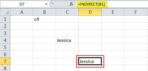
For example, in the next image, cell B1 contains the text string “c4.” Enter the formula “=INDIRECT(B1)” in any cell, e.g., D7. This INDIRECT Excel formula works as follows:
- The INDIRECT function refers to cell B1, which consists of “c4.”
- The INDIRECT function goes to cell C4 and returns its value “Jessica” in cell D7.
In this way, the text string “c4” is converted into the cell address C4. Then, the INDIRECT Excel function heads to this cell address (C4) and returns its value (Jessica).
The INDIRECT function lets the user specify an indirect cell address in the form of a text string. Apart from cells, this function can also refer to named ranges, other workbooks, and worksheets with the help of text strings.
The advantage of using the INDIRECT Excel function is that the indirect references do not change with the insertion or deletion of new rows or columns. Moreover, the user can change the text string (indirect cell address) of the cell referred to in the formula without changing the INDIRECT formula itself.
For instance, in the preceding example, type “c2” (without the double quotation marks) in cell B1 and retain the formula “=INDIRECT(B1).” So, this time the INDIRECT function goes to cell C2 and returns its content. Hence, the text string changed rather than the INDIRECT Excel formula.
Using the INDIRECT Excel function converts text values into valid cell addresses. The INDIRECT function is categorized under the LOOKUP and REFERENCE functions of Excel.
Table of contents
- INDIRECT Function In Excel
- Syntax of the INDIRECT Function
- How to Use the INDIRECT Function in Excel?
- Example #1–Reference to a Named Range
- Example #2–Reference to a Worksheet
- Example #3–Reference to the Last Month (R1C1-Style)
- Example #4–Reference to a Table Array
- Example #5–Reference to a Drop-down List
- How is the A1-Style Different From the R1C1-Style of Referencing?
- The Cautions While Working With the INDIRECT Excel Function
- Frequently Asked Questions
- Recommended Articles
Syntax of the INDIRECT Function
The syntax of the INDIRECT function of Excel is shown in the following image:
The function accepts the following arguments:
- ref_text: This is a cell address or cell referenceCell reference in excel is referring the other cells to a cell to use its values or properties. For instance, if we have data in cell A2 and want to use that in cell A1, use =A2 in cell A1, and this will copy the A2 value in A1.read more. It refers to the cell which contains a text string. This text string is an indirect cell address that we can specify in either the A1-style or the R1C1-style. “Ref_text” can also refer to a cell containing the name of a named range, a workbook, or a worksheet.
- a1: This is a logical (or Boolean) value–true or false. It specifies the style of reference used by the “ref_text” argument. It can take either of the following values:
| a1 | When true or omitted or 1, the “ref_text” argument is considered to be in A1-style. |
| a1 | When false or 0, the “ref_text” argument is considered to be in R1C1-style. |
The argument “ref_text” is mandatory while “a1” is optional.
Note 1: If the text string is entered in R1C1-style reference (like r2c3), it is compulsory to enter the “a1” argument (as 0 or false) in the INDIRECT excel formula.
Note 2: For more on A1-style and R1C1-style references, refer to the topic “how is the A1-style different from the R1C1-style of referencing?” at the end of example #5.
How to Use the INDIRECT Function in Excel?
Let us consider a few examples to understand the working of the INDIRECT function in Excel.
You can download this INDIRECT Function Excel Template here – INDIRECT Function Excel Template
Example #1–Reference to a Named Range
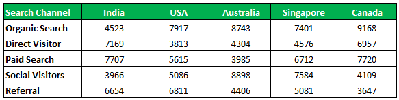
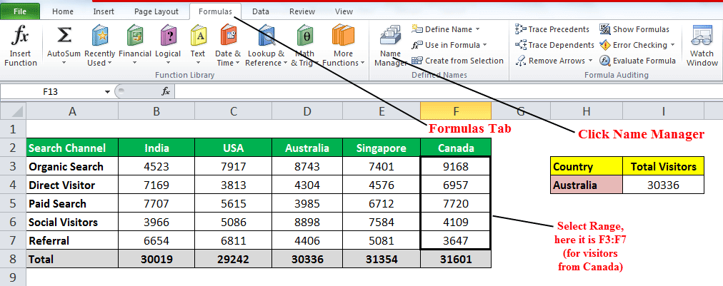
The following table displays the number of visitors to the website www.xyz.com. These visitors have been categorized under different channels. Each channel is listed in the column “Search Channel.”
Further, these visitors belong to five countries: India, the USA, Australia, Singapore, and Canada. Each country is represented by its respective column.
We want to perform the following tasks:
- Calculate the total number of visitors to each country using the SUM functionThe SUM function in excel adds the numerical values in a range of cells. Being categorized under the Math and Trigonometry function, it is entered by typing “=SUM” followed by the values to be summed. The values supplied to the function can be numbers, cell references or ranges.read more.
- Create named rangesName range in Excel is a name given to a range for the future reference. To name a range, first select the range of data and then insert a table to the range, then put a name to the range from the name box on the left-hand side of the window.read more for the figures of each of the five countries. We must call every range according to the country it represents. This range must exclude the totals and the titles of the columns.
- Calculate the total number of visitors from Canada by using the named ranges and the INDIRECT function of Excel.
- Apply the data validationThe data validation in excel helps control the kind of input entered by a user in the worksheet.read more feature of Excel to cell H4. By typing the country’s name in cell H4, cell I4 must show its respective total. Use the named ranges and the INDIRECT Excel function for the same.
The steps to perform the given tasks are listed as follows:
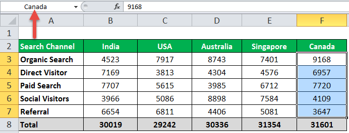
Step 1: In row 8, we must calculate the total visitors of each country by applying the SUM function. The totals of columns B, C, D, E, and F are shown in the next image.
Create a named range for the data of each country. Let us begin by naming the range F3:F7 as “Canada.” For this, perform the following tasks:
a. Select the range F3:F7.
b. In the name box, type “Canada” without the double quotation marks. The name box is to the left of the formula bar and is shown with a red arrow in the next image.
c. Press the “Enter” key.
The range F3:F7 has been named “Canada.”
Note: The names of the named ranges are not case-sensitive. It implies that if a range is called “figures,” the terms “FigUres,” “fIguReS,” etc. mean the same to Excel.
The alternative method to create a named range has been discussed in the following pointers (step 1a to step 1c).
Step 1a: Select the range (F3:F7) to be named.
- Click “Name Manager” from the “Formulas” tab of the Excel ribbon.
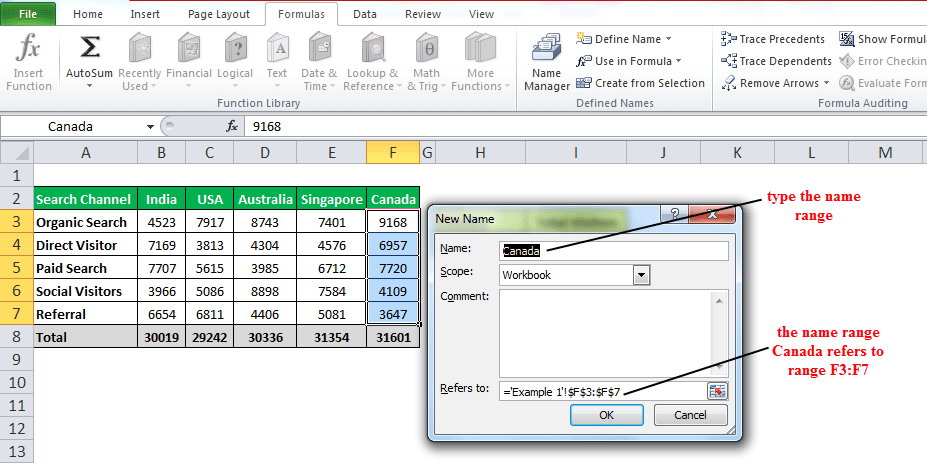
- Click “New.”
Step 1b: The “New Name” box opens. Next, perform the following tasks:
a. In the “Name” box, type “Canada” without the double quotation marks.
b. In “Refers to,” the selected range F3:F7 is displayed. If this range is not showing in the “Refers to” box, select it.
c. Click “OK.” Finally, close the “Name Manager” dialog box.
The selected range (F3:F7) has been named “Canada.” The selection of this range has been shown in the following image and the image under step 1a.
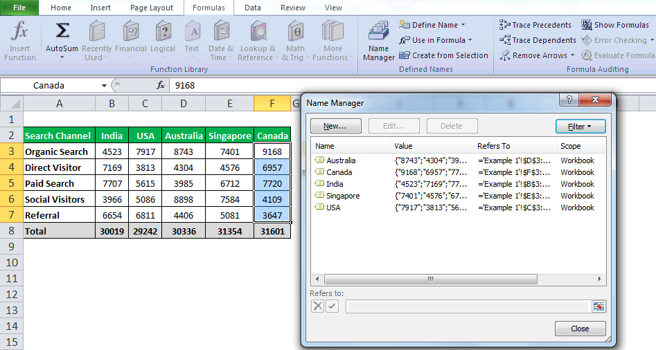
Step 1c: Likewise, we must create named ranges for the numbers of all the five countries. The five named ranges titled Australia (D3:D7), Canada (F3:F7), India (B3:B7), Singapore (E3:E7), and USA (C3:C7) have been created.
The named ranges are shown in the following image.
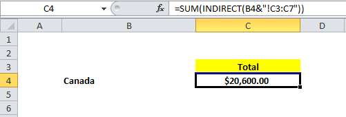
Step 2: To calculate the total number of visitors from Canada, enter the following formula in cell I4.
“=SUM(INDIRECT(H4))”
The INDIRECT Excel function refers to cell H4, which contains the name “Canada.” It goes to the range “Canada” (F3:F7) and returns its total. That is because the INDIRECT function is enclosed within the SUM function.

Step 3: Before applying the data validation feature, a named range consisting of the names of the five countries needs to be created. For this, perform the following tasks in the given sequence:
a. Select “Name Manager” from the “Formulas” tab and click “New.” The “New Name” dialog box opens.
b. In the “Name” box, type “Country” (without the double quotation marks), as shown in the following image.
c. In the “Refers to” box, select the cells B2:F2. Click “Ok.”
d. Close the “Name Manager” window.
A named range titled “Country” is created.

Step 4: Apply the data validationThe data validation in excel helps control the kind of input entered by a user in the worksheet.read more feature to cell H4. For this, perform the following tasks in the stated order:
a. Select the cell (H4) to which we must apply the data validation feature.
b. Click the “Data Validation” drop-down from Excel’s “Data” tab. Select “Data Validation.”
c. The “Data Validation” window opens, as shown in the following image. In the “Settings” tab, select “List” from the “Allow” drop-down.
d. In “Source,” type “=Country” without the double quotation marks.
e. Select “Ignore blank” and “In-cell drop-down ” checkboxes.” Click “OK.”
The data validation feature has been applied to cell H4. Therefore, depending on whether the checkbox of “in-cell dropdown” is selected or not (in step d), a drop-down arrow may or may not appear next to cell H4.
The drop-down arrow does appear next to cell H4, though it has not been shown in the following images. This drop-down arrow (next to cell H4) shows the names of the five countries, India, USA, Australia, Singapore, and Canada.
Note: The data validation feature restricts the input that a user can enter in a cell of a worksheet. It allows the user to enter only those values defined by the data validation rule.

Step 5: Once the data validation feature has been applied, we must enter the name of any of the five countries (India, USA, Australia, Singapore, and Canada) in cell H4. The total number of visitors to the selected country will appear in cell I4.
To insert the name of a country in cell H4, one can either type the required country or select it from the drop-down arrow next to cell H4.
An error message appears if an input other than the names of the given five countries is entered in cell H4. This message states that restrictions have been defined for this cell (H4).
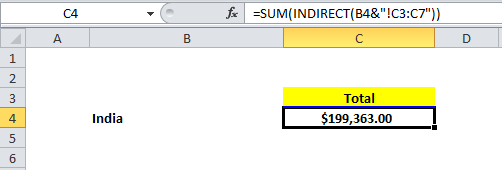
For instance, enter “India” in cell H4. The sum of its visitors (30,019) appears in cell I4. It is shown in the following image.

In the following pointers (step 5a to step 5b), the results of the data validation feature are examined.
Step 5a: Enter “Australia” in cell H4. The total number of visitors (30,336) appears in cell I4. The same is shown in the following image.

Step 5b: Enter “Australia” in cell H4. The total number of visitors (30,336) appears in cell I4. The same is shown in the following image.
Hence, one must note that we did not change the INDIRECT Excel formula of cell I4 to obtain the total visitors of the different countries. We only changed the names of the ranges in cell H4.
Thus, we changed the cell’s content referred to in the formula (H4) without changing the formula itself (in cell I4).

Example #2–Reference to a Worksheet
The next images (image 1, image 2, and image 3) show the sales revenue (in $) generated by the different channels (under “Search Channel”) in other countries. Every channel represents a category of visitors to the website www.xyz.com.
Further, one image has been created in one Excel worksheet. As a result, every worksheet has been named by the country it represents. So, for instance, the worksheet containing the numbers of India has been called “India.”
The total sales revenue of five countries (India, USA, Australia, Singapore, and Canada) has been shared. These totals have been calculated with the SUM function of Excel.
We want to perform the following tasks:
- Calculate the total sales revenue generated by each country using the INDIRECT and the SUM functions.
- Cross-check the results of the INDIRECT function in excel (enclosed within SUM) with the simple SUM function.
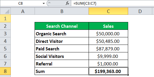
The total sales revenue of Singapore and Canada are $65,358 and $20,600, respectively. For these countries, assume that the sales generated by the different channels are listed in the range C2:C8 of the worksheets titled “Singapore” and “Canada,” respectively. Cell C2 contains the caption “Sales,” and cell C8 has the sum of the range C3:C7 (calculated by the SUM function).
[Please note that the total sales revenues calculated with the SUM function have been shared to enable cross-checking of results.]
Image 1
The total sales revenueSales revenue refers to the income generated by any business entity by selling its goods or providing its services during the normal course of its operations. It is reported annually, quarterly or monthly as the case may be in the business entity’s income statement/profit & loss account.read more (in $) of India is shown in the following image:
[Consider the entire column “search channel” as range B2:B8 of the worksheet “India.” The column “sales” is in the range C2:C8. These ranges also include the titles of the green boxes.]
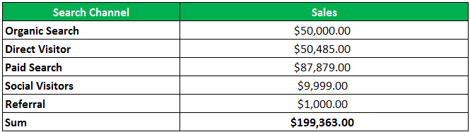
Image 2
The total sales revenue (in $) of the USA is shown in the following image:
[Consider the column “search channel” as range B2:B8 of the worksheet “USA.” The column “sales” is in the range C2:C8.]
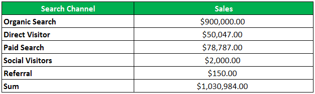
Image 3
The total sales revenue (in $) of Australia is shown in the following image:
[Consider this image as a part of the worksheet titled “Australia.”]
The steps to calculate the total sales revenue of the different countries by using the INDIRECT Excel function are listed as follows:
Step 1: To find the total sales revenue generated by each country, concatenate (join) the name of the worksheet and the channel-wise sales figures (listed in the “sales” column of the preceding images). It is because the sales figures of different countries are in separate worksheets.
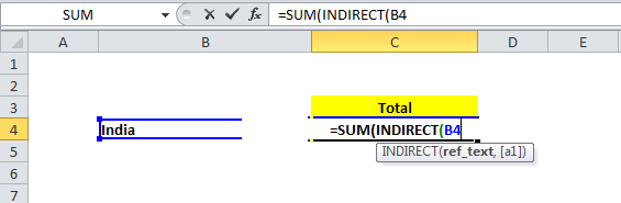
In cell C4, begin typing the following INDIRECT Excel formula.
“=SUM(INDIRECT(B4”
The same is shown in the next image.
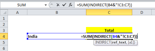
Step 2: Complete the preceding formula (entered in step 1) in cell C4.
“=SUM(INDIRECT(B4&”!C3:C7))”
The same is shown in the following image.
The “ref_text” argument (B4&”!C3:C7) begins with cell B4, which contains “India.” “India” is the name of the worksheet which contains image 1. So, in the first argument of the INDIRECT function, we refer to the worksheet indirectly by its name.
Further, we use the operator ampersand (&) for combining the sheet name (India) in cell B4 and the range to be summed up (C3:C7) in image 1.
Step 3: Press the “Enter” key. The output appears in cell C4, as shown in the following image.
Since the INDIRECT function in excel is enclosed within the SUM function (refer to the formula entered in step 2), the sum of the range C3:C7 of worksheet “India” is returned.
Hence, the total revenue of $199,363 matches the “SUM” amount of image 1. It implies that the result of the preceding formula (in step 2) is the same as that of the simple SUM function (in the second succeeding image).
The application of the SUM function to the range C3:C7 has been shown in the following image to allow cross-checking of results.
In the following pointers (step 3a to step 3c), the total sales revenue of the different countries is examined.
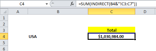
Step 3a: For calculating the total sales revenue of the USA, perform the following tasks:
- Enter “USA” (without the double quotation marks) in cell B4.
- Enter the formula “=SUM(INDIRECT(B4&”!C3:C7))” in cell C4.
- Press the “Enter” key.
In the given INDIRECT Excel formula, the value of cell B4 (worksheet named “USA”) is joined with the range (C3:C7 of image 2) to be summed.
Hence, the total revenue of $1,030,984 appears in cell C4. This number is the same as the “sum” amount of image 2.
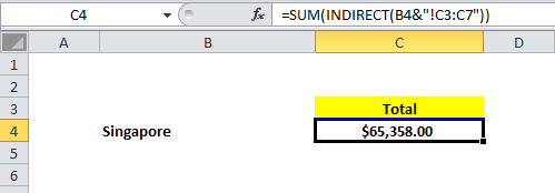
Step 3b: Enter “Singapore” in cell B4. The formula to be entered in cell C4 remains the same as in the preceding step (step 3a).
Press the “Enter” key. The output of $65,358 appears in cell C4, as shown in the following image.
Step 3c: Enter “Canada” in cell B4. Retain the same formula as the preceding step (step 3a).
The output in cell C4 is $20,600.
Likewise, we can calculate the total sales revenue of Australia by entering the respective name in cell B4 and retaining the formula of cell C4.
Hence, by changing the sheet names (in cell B4) and retaining the formula (in cell C4), we have obtained the total sales revenue of the different countries. Please note that we made no changes to the INDIRECT formula (in cell C4).
Thus, we changed the values of the first argument, “ref_text” (different sheet names), though the cell address of the INDIRECT excel formula remains the same (B4).
Example #3–Reference to the Last Month (R1C1-Style)
The next images (image 1, image 2, and image 3) show the sales revenue (in $) generated by the different channels (under “search channel”) in the first three months of 2018. The entire data relates to the website www.xyz.com.
We want to perform the following tasks:
- Find out the total sales revenue of the last month (March) by using the R1C1 reference style of the INDIRECT function in excel.
- Add a fifth column (column E) to the existing dataset, which contains the sales of April. Find out the total sales revenue of the last added month (April) by using the R1C1-style of the INDIRECT function.
- Cross-check the output of the INDIRECT formulas with the totals of the respective months. These totals have been calculated with the help of the SUM function of Excel.
The figures of April are–$12,943 (organic search), $7,279 (direct visitor), $7,889 (paid search), $10,327 (social visitors), $2,154 (referral), and $40,592 (total).
Image 1
The channel-wise sales revenues (in $) for January, February, and March are shown in the following image:
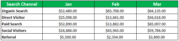
Image 2
The total sales revenue ($) for January, February, and March are shown in the following image:
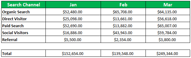
Image 3
The total sales revenues of March and April are to be calculated in the cell B13 (containing a question mark) shown in the following image:

The steps to perform the given tasks are listed as follows:
Step 1: Begin by entering the following formula in cell B13.
“=INDIRECT(“R10C”&COUNTA(10:10))”
The same is shown in the following image.

Step 2: Complete the preceding formula (step 1) in cell B13.
“=INDIRECT(“R10C”&COUNTA(10:10),FALSE)”
The same is shown in the following image.
The first argument of the INDIRECT excel function is “R10C”&COUNTA(10:10). In this argument, we have concatenated R10C and the COUNTA functionThe COUNTA function is an inbuilt statistical excel function that counts the number of non-blank cells (not empty) in a cell range or the cell reference. For example, cells A1 and A3 contain values but, cell A2 is empty. The formula “=COUNTA(A1,A2,A3)” returns 2.
read more with the help of the operator “&.” The COUNTA function counts the total number of non-empty cells in row 10. It returns 4.
So, R10C joined with 4 results in the cell number R10C4. Since the second argument of the INDIRECT function is “FALSE,” R10C4 is recognized as an R1C1-style reference by Excel.
Note: For more on R1C1-style references, refer to the topic “how is the A1-style different from the R1C1-style of referencing?” at the end of example #5.

Step 3: Press the “Enter” key. Since the “ref_text” argument evaluates to R10C4, the INDIRECT Excel formula returns the cell value at the intersection of row 10 and column 4. In the A1-style, this is cell D10 of Excel.
Hence, the output is $249,344.

Step 4: Add the sales figures for April in column E of the existing dataset. Enter the following formula in cell B13.
“=INDIRECT(“R10C”&COUNTA(10:10),FALSE)”
The first argument of the INDIRECT Excel function is “R10C”&COUNTA(10:10), and the second argument is “FALSE”. The COUNTA function returns the value 5 as there are five non-empty cells in row 10.
When R10C is joined with 5, it results in R10C5. This R10C5 is the R1C1-style reference which implies cell E10 (A1-style). The row number is 10, and the column number is 5 (column E).
Hence, the INDIRECT Excel formula returns the value of cell E10. So, the total sales revenue for April is $40,592.

Likewise, we can add the sales data for the remaining months to the existing dataset. Then, with the same INDIRECT formula (entered in steps 2 and 4), we can obtain the total sales revenues of the last added month.
One can notice that even after adding the data for April, the INDIRECT Excel formula remained the same. In other words, the INDIRECT formula we used for calculating the sales revenue for March is the same as that of April.
The INDIRECT formula did not change because it perceives “R10C” in the “ref_text” argument as a text string.
Hence, the indirect references do not change with the insertion or deletion of new rows or columns in Excel.
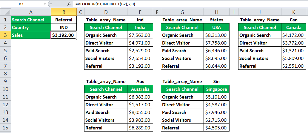
Example #4–Reference to a Table Array
The following image contains five table arrays. Each array includes the sales revenue generated from the different visitor channels (under “search channel”) of a website (www.xyz.com).
One table array represents the data of one country. For the five countries, India, USA, Canada, Australia, and Singapore, the table arrays are named “Ind,” “States,” “Can,” “Aus,” and “Sin,” respectively.
In addition, the entire range of every table array is a named range. The name of the range is the same as the name of the table array. For instance, the range D2:E7 has been called “Ind,” G2:H7 has been named “States,” and so on.
We want to perform the following tasks:
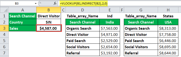
- Obtain the sales of the “Direct Visitor” channel of Singapore (in cell B3) with the help of the VLOOKUP functionThe VLOOKUP excel function searches for a particular value and returns a corresponding match based on a unique identifier. A unique identifier is uniquely associated with all the records of the database. For instance, employee ID, student roll number, customer contact number, seller email address, etc., are unique identifiers.
read more of Excel. - Obtain the sales of Singapore’s “Direct Visitor” channel (in cell B3) by using a combination of the VLOOKUP and INDIRECT functions.
- Obtain the sales of India’s “Referral” channel (in cell B3) by using a combination of the VLOOKUP and INDIRECT Excel functions.
One can cross-check the output of the preceding pointers with the figures of the respective table arrays.

The steps to perform the given tasks are listed as follows:
Step 1: To obtain the sales of the “Direct Visitor” channel of Singapore by the VLOOKUP function, perform the following tasks:
a. Enter “direct visitor” (without the double quotation marks) in cell B1.
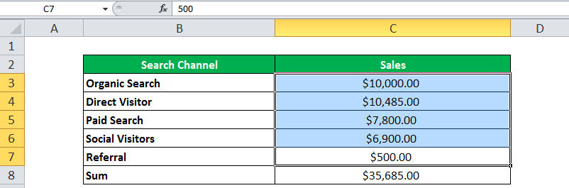
b. Ensure that the range G10:H15 is named “Sin.” Thereafter, enter “Sin” in cell B2.
c. Enter the formula “=VLOOKUP(B1,B2,2,0)” in cell B3.
d. Press the “Enter” key.
The output “N/A” error appears in cell B3, as shown in the following image.
The “N/A” error appears because we have mistakenly entered the “table_array” argument (second argument) as “B2.” Unfortunately, the VLOOKUP function could not recognize this argument (B2). The “table_array” argument is always entered as a range of cells.
Hence, an incorrect argument makes the VLOOKUP formula return an error.
Had we entered the VLOOKUP formula as: “=VLOOKUP(B1,G10:H15,2,0)” in cell B3, the output would have been $4,587.

Step 2: To obtain the sales of the “Direct Visitor” channel of Singapore by a combination of the VLOOKUP and INDIRECT functions, perform the following tasks:
- Enter “Direct Visitor” in cell B1 and “Sin” in cell B2. The range G10:H15 has already been named “Sin” in the preceding step (step 1).
- Enter the formula “=VLOOKUP(B1,INDIRECT(B2),2,0)” in cell B3, as shown in the following image.
The first argument, cell B1 is the “lookup_value” of the VLOOKUP function. So, this function searches for the string “Direct Visitor.”
The INDIRECT excel function refers to cell B2, which contains “Sin.” This “Sin” is the “table_array” argument of the VLOOKUP function. The VLOOKUP function searches for the string “direct visitor” in the range “Sin” (G10:H15).
Further, the “col_index_num” argument is 2. So, the VLOOKUP function searches for the lookup value (direct visitor) in the second column of the range “Sin.”
Since the fourth argument (range_lookup) is 0, the given VLOOKUP formula returns an exact match. An exact match is a value equal to the lookup value.

Step 3: Press the “Enter” key. The output of $4,587 appears in cell B3. This output matches the value of cell H12 which is a part of the table array of Singapore.
Hence, the preceding formula (entered in step 2) has returned the sales of Singapore’s “Direct Visitor” channel.
Step 4: To obtain the sales of the “Referral” channel of India with the help of the VLOOKUP and INDIRECT functions, perform the following tasks in the stated order:
- Enter “referral” in cell B1 and “Ind” in cell B2.
- Ensure that the range D2:E7 is named “Ind.”
- Enter the formula “=VLOOKUP(B1,INDIRECT(B2),2,0)” in cell B3.
- Press the “Enter” key.
The output appears in cell B3, as shown in the succeeding image.
We have changed the values of cells B1 and B2 to “Referral” and “Ind,” respectively. Since named ranges are not case-sensitive, “IND” and “Ind” mean the same to Excel.
The first argument (lookup_value) of the VLOOKUP is “B1.” The output of “INDIRECT(B2)” works as the “table_array” argument of the VLOOKUP function. The “col_index_num” argument is 2. The “range_lookup” argument is 0 or false (exact match).
The VLOOKUP searches for the value “referral” in the named range “Ind” (D2:E7). It returns an exact match from the second column of the range “Ind.”
Hence, India’s “Referral” channel sales are $3,192. This output does match with the value of cell E7. This cell is a part of the table array of the country India.
Likewise, we can change the values of cells B1 and B2 to obtain the different sales numbers in cell B3.
We must note that the formulas entered in steps 2 and 4 are the same. Therefore, retain this formula to obtain the required sales figures in cell B3. Next, we must change the values of cells B1 and B2 according to the output required in cell B3.
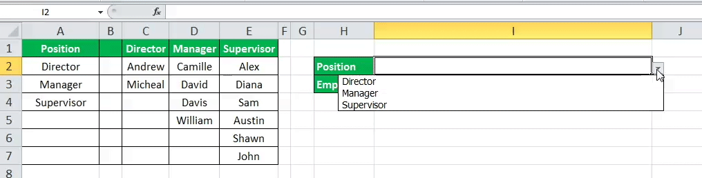
Example #5–Reference to a Drop-down List
The following image shows three designations (director, manager, and supervisor) prevalent in an organization. These positions (designations or ranks) are listed in column A. Columns C, D, and E state the names of those employees who are currently serving in these positions.
We want to perform the following tasks:
- Create a drop-down list in cell I2. When the drop-down arrow is clicked, the list must display the names of the three positions (Director, Manager, and Supervisor).
- Create a dependent drop-down list in cell I3. As a position is typed in cell I2, the corresponding names of employees (serving at that position) should be displayed. For instance, if “Director” is typed in cell I2, cell I3 should show the names of the Directors (listed in column C) of the organization.
Use the named ranges, data validation feature, and the INDIRECT function of Excel.

The steps to perform the given tasks are listed as follows:
Step 1: Name the ranges of the given dataset. For naming the ranges, select the range and type the required name in the name box (refer to step 1 of example #1).
The ranges should be named as follows:
- Name the range A2:A4 as “Position.”
- Name the range C2:C3 as “Director.”
- Name the range D2:D5 as “Manager.”
- Name the range E2:E7 as “Supervisor.”
Note:While naming the ranges, do not enter the beginning and the ending double quotation marks (shown in the preceding pointers) in the name box.
Step 2: For creating a drop-down list in cell I2, perform the following steps:
- Select cell I2. Click the “Data Validation” drop-down from the “Data” tab of Excel. Select “Data Validation.”
- In the settings tab of the “Data Validation” window, select “List” under the “Allow” drop-down.
- Under “Source,” Type “Position” (without the double quotation marks).
- Select the checkboxes of “ignore blank” and “in-cell dropdown.”
A drop-down list is created in cell I2, as shown in the following image. When the drop-down arrow (next to cell I2) is clicked, the names of the three positions (director, manager, and supervisor) appear.
To enter a position in cell I2, one can either type it or select it from the drop-down list.
Step 3: To create a dependent drop-down list in cell I3, we need to apply the data validation feature to the given cell. For this, perform the following steps:
Select cell I3. Click the “Data Validation” drop-down from the “Data” tab of the Excel ribbon.
b. Select “Data Validation.” The “Data Validation” window opens.
c. In the “Settings” tab, select “List” under “Allow.”
d. Select the checkboxes of “Ignore blank” and “In-cell dropdown” if they are not selected.
e. Under “Source,” enter the formula “=INDIRECT($I$2)” without the double quotation marks. Click “OK.”
The same is shown in the following image. Once “OK” is clicked (in step e), the drop-down arrow appears in cell I3.
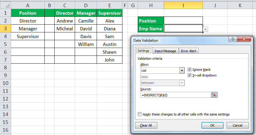
In the following pointers (step 3a to step 3c), the different drop-down lists (in cell I3) that appear on typing the position (in cell I2) have been examined.
Step 3a: Type “Director” (without the double quotation marks) in cell I2. Clicking the drop-down arrow of cell I3 displays the names of employees, Andrew and Micheal. These employees are serving in the mentioned position.
The same is shown in the following image.
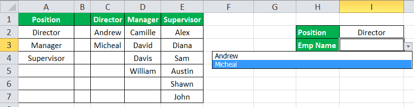
Step 3b: Type “Manager” (without the double quotation marks) in cell I2. The drop-down of cell I3 displays the names Camille, David, Davis, and William. These employees are the managers of the organization.
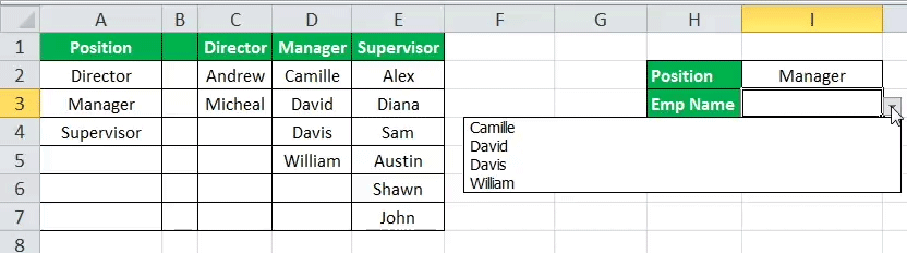
Step 3c: Type “Supervisor” (without the double quotation marks) in cell I2. The drop-down of cell I3 displays the names of the employees working as supervisors in the organization: Alex, Diana, Sam, Austin, Shawn, and John.

We must note that the drop-down list of cell I3 is dependent on cell I2. Therefore, it implies that cell I3 displays the names of employees corresponding to the name of the position typed in cell I2.
Before creating a dependent drop-down list (in cell I3), ensure that all ranges (in columns A, C, D, and E) are named and after that, apply the data validation feature to cell I3.
How is the A1-Style Different From the R1C1-Style of Referencing?
In the A1-style of referencing, every cell address consists of a column letter followed by a row number. For instance, address C5 refers to the cell at the intersection of column C and row 5.
In the A1-style referencing, every cell address consists of a column letter followed by a row number. For instance, address C5 refers to the cell at the intersection of column C and row 5.
On the other hand, in the R1C1-style, a cell address consists of a row number followed by a column number. Instead of letters, every column has a unique number assigned to it. For instance, cell A2 in A1-style is called R2C1 in R1C1-style.
To change the Excel reference style from A1 to R1C1, perform the following steps:
- From the File tab of Excel, click “options.”
- The “Excel Options” window opens. Select “Formulas.”
- Under “Working with formulas,” select the checkbox of “R1C1 reference style.”
- Click “OK.”
Consequently, all the column letters will change to numbers. Moreover, if there are any formulas in the worksheet, their cell references will adjust according to the R1C1-style.
By default, the INDIRECT function of Excel uses the A1-style of referencing. However, we can change the referencing style to R1C1 by entering “0” or “False” in the “a1” argument.
The Cautions While Working With the INDIRECT Excel Function
The cautions to be observed while working with the INDIRECT function of Excel are listed as follows:
- The “ref_text” argument must be a valid cell reference. If not, the INDIRECT function will return the “#REF!” error.
- The “ref_text” argument can refer to another workbook (an external reference). Ensure that the concerned workbook (source workbook) is open. If not, the INDIRECT function will return the “#REF!” error.
- The “ref_text” argument must not refer to a cell range beyond the maximum of 1,048,576 rows or 16,384 columns (XFD). The INDIRECT function in excel returns a “#REF!” error if it does.
The “#REF!” error is shown in the following image.
Note: In the modern versions of Excel, XFD is the right-most column of a worksheet.
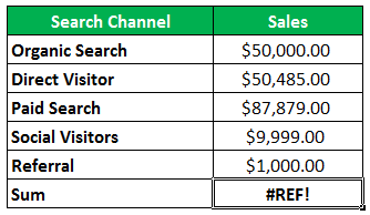
Frequently Asked Questions
1. Define the INDIRECT function of Excel.
The INDIRECT function returns the value of a cell whose address is provided by a text string. In other words, the function can interpret text strings as valid cell addresses (or cell references). Once analyzed, the function goes to this cell address, picks its value, and returns it.
The INDIRECT function does not perform any calculations. It just evaluates a reference and displays its content. The text string (or the reference) entered in the function can be changed without changing the INDIRECT formula.
The syntax of the INDIRECT function of Excel is stated as follows:
“INDIRECT(ref_text,[a1])”
The “ref_text” argument is the cell address that contains a text string, a named range, or the name of a worksheet or workbook.
The “a1” argument is the value true or false. If “a1” is true or 1 (or omitted), the “ref_text” argument is treated as an A1-style reference. If “a1” is false or 0, the “ref_text” argument is considered in R1C1-style.
2. How should the INDIRECT function be used with the data validation feature of Excel?
With the help of the INDIRECT function and the data validation feature, it is possible to create dependent drop-down lists. A dependent drop-down list displays a series of items depending on selecting a value in another cell.
For example, there are two lists titled “flowers” and “trees” in an Excel worksheet. First, let us create a dependent drop-down list in cell E3. This list should be dependent on the value entered in cell E2.
The text “flowers” is displayed in cell A1. This list contains the following items:
• Cell A2 contains Rose
• Cell A3 contains Lotus
• Cell A4 contains Sunflower
• Cell A5 contains Tulip
The text “trees” is shown in cell B1. This list contains the following items:
• Cell B2 contains Oak
• Cell B3 contains Pine
• Cell B4 contains Maple
• Cell B5 contains Spruce
The steps to create a drop-down list in cell E3, which depends on cell E2, are listed as follows:
a. Name the range A2:A5 as “Flowers” and B2:B5 as “Trees.”
b. Select cell E3.
c. Click the “Data Validation” drop-down from the “Data” tab of Excel. Select “Data Validation.”
d. In the “Settings” tab, select “List” under the “Allow” drop-down.
e. Under the “Source” drop-down, enter the formula “=INDIRECT($E$2).” The list (of cell E3) should depend on the value selected in cell E2.
f. Select the two checkboxes of “Ignore blank” and “In-cell dropdown.” Click “OK.”
A dependent drop-down list is created in cell E3.
When “Flowers” is typed in cell E2, the drop-down arrow next to E3 displays the list–Rose, Lotus, Sunflower, and Tulip. Similarly, if “Trees” is typed in cell E2, cell E3 shows the Oak, Pine, Maple, and Spruce values.
Note: Please do not enter the double quotation marks in the name of the range (in step a) and the INDIRECT Excel formula (in step d).
3. Why and when should the INDIRECT function be used in Excel?
We should use the INDIRECT function of Excel for the following reasons:
a. It helps indirectly refer to a cell, range, worksheet, or workbook.
b. It allows fixing a reference to not change with the insertion or deletion of rows or columns.
c. It helps obtain different outputs by changing the text string to which the INDIRECT formula refers.
We should use the INDIRECT function of Excel in the following situations:
a. It is used when there is a need to create dynamic cell references. For making a dynamic reference to a range, enter its name in a cell, and refer to that cell in the INDIRECT formula [like “=INDIRECT(C1)” where the cell C1 contains the name of the range].
b. It is used when there is a need to convert a text string into a valid cell address. The text string supplied to the function can be changed as per the user requirement without changing the actual INDIRECT formula.
c. It is used when there is a need to lock a cell reference. A cell reference is locked to prevent it from changing with the insertion or deletion of rows or columns. For instance, the formula “=INDIRECT(“B2”)” identifies “B2” as a text string rather than a cell reference. The string “B2” remains intact with the insertion of a row preceding cell B2 (like row 1).
Recommended Articles
This article is a guide to the INDIRECT Excel function. Here we discuss how to use an INDIRECT formula in Excel and step-by-step examples. Take a look at the following articles in Excel: –
- Indirect Labor Example
- Excel Check Mark
- Excel Indirect Formula
- Name Manager in Excel