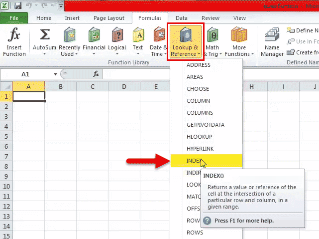
What is index function in excel - Word и Excel - помощь в работе с программами

The INDEX function returns a value or the reference to a value from within a table or range.

There are two ways to use the INDEX function:

If you want to return the value of a specified cell or array of cells, see Array form.
If you want to return a reference to specified cells, see Reference form.

Array form

Description

Returns the value of an element in a table or an array, selected by the row and column number indexes.

Use the array form if the first argument to INDEX is an array constant.

Syntax

INDEX(array, row_num, [column_num])

The array form of the INDEX function has the following arguments:

array Required. A range of cells or an array constant.
- If array contains only one row or column, the corresponding row_num or column_num argument is optional.
- If array has more than one row and more than one column, and only row_num or column_num is used, INDEX returns an array of the entire row or column in array.
row_num Required, unless column_num is present. Selects the row in array from which to return a value. If row_num is omitted, column_num is required.
column_num Optional. Selects the column in array from which to return a value. If column_num is omitted, row_num is required.

Remarks

If both the row_num and column_num arguments are used, INDEX returns the value in the cell at the intersection of row_num and column_num.
row_num and column_num must point to a cell within array; otherwise, INDEX returns a #REF! error.
If you set row_num or column_num to 0 (zero), INDEX returns the array of values for the entire column or row, respectively. To use values returned as an array, enter the INDEX function as an array formula.

Note: If you have a current version of Microsoft 365, then you can input the formula in the top-left-cell of the output range, then press ENTER to confirm the formula as a dynamic array formula. Otherwise, the formula must be entered as a legacy array formula by first selecting the output range, input the formula in the top-left-cell of the output range, then press CTRL+SHIFT+ENTER to confirm it. Excel inserts curly brackets at the beginning and end of the formula for you. For more information on array formulas, see Guidelines and examples of array formulas.

Examples

Example 1

These examples use the INDEX function to find the value in the intersecting cell where a row and a column meet.

Copy the example data in the following table, and paste it in cell A1 of a new Excel worksheet. For formulas to show results, select them, press F2, and then press Enter.

Data	Data
Apples	Lemons
Bananas	Pears
Formula	Description	Result
=INDEX(A2:B3,2,2)	Value at the intersection of the second row and second column in the range A2:B3.	Pears
=INDEX(A2:B3,2,1)	Value at the intersection of the second row and first column in the range A2:B3.	Bananas

Example 2

This example uses the INDEX function in an array formula to find the values in two cells specified in a 2×2 array.

Note: If you have a current version of Microsoft 365, then you can input the formula in the top-left-cell of the output range, then press ENTER to confirm the formula as a dynamic array formula. Otherwise, the formula must be entered as a legacy array formula by first selecting two blank cells, input the formula in the top-left-cell of the output range, then press CTRL+SHIFT+ENTER to confirm it. Excel inserts curly brackets at the beginning and end of the formula for you. For more information on array formulas, see Guidelines and examples of array formulas.

Formula	Description	Result
=INDEX({1,2;3,4},0,2)	Value found in the first row, second column in the array. The array contains 1 and 2 in the first row and 3 and 4 in the second row.	2
	Value found in the second row, second column in the array (same array as above).	4

Top of Page

Reference form

Description

Returns the reference of the cell at the intersection of a particular row and column. If the reference is made up of non-adjacent selections, you can pick the selection to look in.

Syntax

INDEX(reference, row_num, [column_num], [area_num])

The reference form of the INDEX function has the following arguments:

reference Required. A reference to one or more cell ranges.
- If you are entering a non-adjacent range for the reference, enclose reference in parentheses.
- If each area in reference contains only one row or column, the row_num or column_num argument, respectively, is optional. For example, for a single row reference, use INDEX(reference,,column_num).
row_num Required. The number of the row in reference from which to return a reference.
column_num Optional. The number of the column in reference from which to return a reference.
area_num Optional. Selects a range in reference from which to return the intersection of row_num and column_num. The first area selected or entered is numbered 1, the second is 2, and so on. If area_num is omitted, INDEX uses area 1. The areas listed here must all be located on one sheet. If you specify areas that are not on the same sheet as each other, it will cause a #VALUE! error. If you need to use ranges that are located on different sheets from each other, it is recommended that you use the array form of the INDEX function, and use another function to calculate the range that makes up the array. For example, you could use the CHOOSE function to calculate which range will be used.

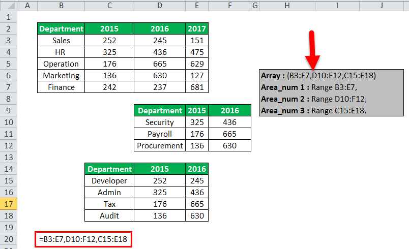
For example, if Reference describes the cells (A1:B4,D1:E4,G1:H4), area_num 1 is the range A1:B4, area_num 2 is the range D1:E4, and area_num 3 is the range G1:H4.

Remarks

After reference and area_num have selected a particular range, row_num and column_num select a particular cell: row_num 1 is the first row in the range, column_num 1 is the first column, and so on. The reference returned by INDEX is the intersection of row_num and column_num.
If you set row_num or column_num to 0 (zero), INDEX returns the reference for the entire column or row, respectively.
row_num, column_num, and area_num must point to a cell within reference; otherwise, INDEX returns a #REF! error. If row_num and column_num are omitted, INDEX returns the area in reference specified by area_num.
The result of the INDEX function is a reference and is interpreted as such by other formulas. Depending on the formula, the return value of INDEX may be used as a reference or as a value. For example, the formula CELL(«width»,INDEX(A1:B2,1,2)) is equivalent to CELL(«width»,B1). The CELL function uses the return value of INDEX as a cell reference. On the other hand, a formula such as 2*INDEX(A1:B2,1,2) translates the return value of INDEX into the number in cell B1.

Examples

Copy the example data in the following table, and paste it in cell A1 of a new Excel worksheet. For formulas to show results, select them, press F2, and then press Enter.

Fruit	Price	Count
Apples	$0.69	40
Bananas	$0.34	38
Lemons	$0.55	15
Oranges	$0.25	25
Pears	$0.59	40

Almonds	$2.80	10
Cashews	$3.55	16
Peanuts	$1.25	20
Walnuts	$1.75	12
Formula	Description	Result
=INDEX(A2:C6, 2, 3)	The intersection of the second row and third column in the range A2:C6, which is the contents of cell C3.	38
=INDEX((A1:C6, A8:C11), 2, 2, 2)	The intersection of the second row and second column in the second area of A8:C11, which is the contents of cell B9.	1.25
=SUM(INDEX(A1:C11, 0, 3, 1))	The sum of the third column in the first area of the range A1:C11, which is the sum of C1:C11.	216
=SUM(B2:INDEX(A2:C6, 5, 2))	The sum of the range starting at B2, and ending at the intersection of the fifth row and the second column of the range A2:A6, which is the sum of B2:B6.	2.42

Top of Page

Is INDEX better than Vlookup?

With sorted data and an approximate match, INDEX-MATCH is about 30% faster than VLOOKUP. With sorted data and a fast technique to find an exact match, INDEX-MATCH is about 13% faster than VLOOKUP.If you use VLOOKUP you must look up the same SKU for each column of information you need.

How do I INDEX an Excel spreadsheet?

To create the index, follow these steps:

Insert a new worksheet at the beginning of your workbook and rename it Index.
Right-click on the sheet tab and select View Code.
Enter the following code in Listing A.
Press [Alt][Q] and save the workbook.

Is INDEX a match?

The INDEX MATCH formula is the combination of two functions in Excel.Combined, the two formulas can look up and return the value of a cell in a table based on vertical and horizontal criteria. For short, this is referred to as just the Index Match function.

What is the difference between INDEX and match in Excel?

The INDEX function can return an item from a specific position in a list. The MATCH function can return the position of a value in a list. The INDEX / MATCH functions can be used together, as a flexible and powerful tool for extracting data from a table.

What is a index sheet?

The INDEX function in Google Sheets returns the value of a cell within an input range, relatively separated from the first cell by row and column offsets. This is similar to the index at the end of a book, which provides a quick way to locate specific content.

How do you calculate the index?

Calculate the index by dividing the current-year result of 0.687 by the previous year result of 0.667 to yield an index of 1.032.

How do you create an index?

Create the index

Click where you want to add the index.
On the References tab, in the Index group, click Insert Index.
In the Index dialog box, you can choose the format for text entries, page numbers, tabs, and leader characters.
You can change the overall look of the index by choosing from the Formats dropdown menu.

How do I use index function instead of VLOOKUP?

Why use INDEX MATCH instead of VLOOKUP?

To get the same result using INDEX MATCH, you need to apply the formula =INDEX($C$2:$C$9,MATCH(F2,$A$2:$A$9,0)) to cell G2.
Using INDEX MATCH will always return the price even after adding/deleting rows as you are using a dynamic reference.

Why do we use index match in Excel?

The INDEX MATCH function is one of Excel’s most powerful features. The older brother of the much-used VLOOKUP , INDEX MATCH allows you to look up values in a table based off of other rows and columns. And, unlike VLOOKUP , it can be used on rows, columns, or both at the same time.

What is VLOOKUP in Excel?

VLOOKUP stands for ‘Vertical Lookup’. It is a function that makes Excel search for a certain value in a column (the so called ‘table array’), in order to return a value from a different column in the same row.

Is index match faster than Xlookup?

We’ve seen that INDEX/MATCH is much faster than XLOOKUP. The same seems to be true for INDEX/MATCH/MATCH in comparison with a 2D XLOOKUP. INDEX/MATCH/MATCH calculates around 30% faster than a 2D XLOOKUP in our test workbook.

Does index match use less memory than Vlookup?

I recommend using INDEX and MATCH. VLOOKUP is slightly faster (approx. 5%), simpler and uses less memory than a combination of MATCH and INDEX or OFFSET. However the additional flexibility offered by MATCH and INDEX often allows you to make significant timesaving compared to VLOOKUP.

What is an index example?

The definition of an index is a guide, list or sign, or a number used to measure change. An example of an index is a list of employee names, addresses and phone numbers.

How do you use index function in sheets?

In Google Sheets, the formula INDEX() allows you to return the value of a cell by specifying which row and column to look at in the specified array. =INDEX(A:A,1,1) for example will always return the first cell in column A.

How do I create an index link in Excel?

Simply select the cell, and then Insert > Hyperlink. This brings up the Insert Hyperlink dialog box, pictured below. To set up a link to another sheet or named reference within the workbook, simply click Place in This Document from the Link to panel.

How do you calculate an index example?

To calculate the percent change between two non-base index numbers, subtract the second index from the first, divide the result by the first index and then multiply by 100. In the example, if the third-year index was 119.1, subtract 114.6 from 119.1 and divide by 114.6.

How do I index a document?

To index a document:

Select a document to index.
In the Document Profile field, select a document profile that matches the type of document to index.
Complete the required metadata fields.
Repeat steps 1 through 3 to index each document in a batch.

Where is the index page of a document?

An index can usually be found at the end of a document, listing the key words and phrases in a document, along with the page numbers they appear on.

Is primary key an index?

A primary key is a special kind of index in that: there can be only one; it cannot be nullable; and. it must be unique.

Does index match work in Google Sheets?

Case-sensitive v-lookup with INDEX MATCH in Google Sheets
VLOOKUP will return the first name it finds no matter its case. Luckily, INDEX MATCH for Google Sheets can do it correctly. You’ll just need to use one additional function — FIND or EXACT.

Источник

The INDEX function returns the value at a given location in a range or array. INDEX is a powerful and versatile function. You can use INDEX to retrieve individual values, or entire rows and columns. INDEX is frequently used together with the MATCH function. In this scenario, the MATCH function locates and feeds a position to the INDEX function, and INDEX returns the value at that position.

In the most common usage, INDEX takes three arguments: array, row_num, and col_num. Array is the range or array from which to retrieve values. Row_num is the row number from which to retrieve a value, and col_num is the column number at which to retrieve a value. Col_num is optional and not needed when array is one-dimensional.

In the example shown above, the goal is to get the diameter of the planet Jupiter. Because Jupiter is the fifth planet in the list, and Diameter is the third column, the formula in G7 is:

=INDEX(B5:E13,5,3) // diameter of Jupiter

The formula above is of limited value because the row number and column number have been hard-coded. Typically, the MATCH function would be used inside INDEX to provide these numbers. For a detailed explanation with many examples, see: How to use INDEX and MATCH.

Basic usage

INDEX gets a value at a given location in a range of cells based on numeric position. When the range is one-dimensional, you only need to supply a row number. When the range is two-dimensional, you’ll need to supply both the row and column number. For example, to get the third item from the one-dimensional range A1:A5:

=INDEX(A1:A5,3) // returns value in A3

The formulas below show how INDEX can be used to get a value from a two-dimensional range:

=INDEX(A1:B5,2,2) // returns value in B2
=INDEX(A1:B5,3,1) // returns value in A3

INDEX and MATCH

In the examples above, the position is «hardcoded». Typically, the MATCH function is used to find positions for INDEX. For example, in the screen below, the MATCH function is used to locate «Mars» (G6) in row 3 and feed that position to INDEX. The formula in G7 is:

=INDEX(B5:E13,MATCH(G6,B5:B13,0),3)

MATCH provides the row number (4) to INDEX. The column number is still hardcoded as 3.

INDEX and MATCH with horizontal table

In the screen below, the table above has been transposed horizontally. The MATCH function returns the column number (4) and the row number is hardcoded as 2. The formula in C10 is:

=INDEX(C4:K6,2,MATCH(C9,C4:K4,0))

For a detailed explanation with many examples, see: How to use INDEX and MATCH

Entire row / column

INDEX can be used to return entire columns or rows like this:

=INDEX(range,0,n) // entire column
=INDEX(range,n,0) // entire row

where n represents the number of the column or row to return. This example shows a practical application of this idea.

Reference as result

It’s important to note that the INDEX function returns a reference as a result. For example, in the following formula, INDEX returns A2:

=INDEX(A1:A5,2) // returns A2

In a typical formula, you’ll see the value in cell A2 as the result, so it’s not obvious that INDEX is returning a reference. However, this is a useful feature in formulas like this one, which uses INDEX to create a dynamic named range. You can use the CELL function to report the reference returned by INDEX.

Two forms

The INDEX function has two forms: array and reference. Both forms have the same behavior – INDEX returns a reference in an array based on a given row and column location. The difference is that the reference form of INDEX allows more than one array, along with an optional argument to select which array should be used. Most formulas use the array form of INDEX, but both forms are discussed below.

Array form

In the array form of INDEX, the first parameter is an array, which is supplied as a range of cells or an array constant. The syntax for the array form of INDEX is:

INDEX(array,row_num,[col_num])

If both row_num and col_num are supplied, INDEX returns the value in the cell at the intersection of row_num and col_num.
If row_num is set to zero, INDEX returns an array of values for an entire column. To use these array values, you can enter the INDEX function as an array formula in horizontal range, or feed the array into another function.
If col_num is set to zero, INDEX returns an array of values for an entire row. To use these array values, you can enter the INDEX function as an array formula in vertical range, or feed the array into another function.

Reference form

In the reference form of INDEX, the first parameter is a reference to one or more ranges, and a fourth optional argument, area_num, is provided to select the appropriate range. The syntax for the reference form of INDEX is:

INDEX(reference,row_num,[col_num],[area_num])

Just like the array form of INDEX, the reference form of INDEX returns the reference of the cell at the intersection row_num and col_num. The difference is that the reference argument contains more than one range, and area_num selects which range should be used. The area_num is argument is supplied as a number that acts like a numeric index. The first array inside reference is 1, the second array is 2, and so on.

For example, in the formula below, area_num is supplied as 2, which refers to the range A7:C10:

=INDEX((A1:C5,A7:C10),1,3,2)

In the above formula, INDEX will return the value at row 1 and column 3 of A7:C10.

Multiple ranges in reference are separated by commas and enclosed in parentheses.
All ranges must on one sheet or INDEX will return a #VALUE error. Use the CHOOSE function as a workaround.

Источник

This Excel tutorial explains how to use the Excel INDEX function with syntax and examples.

Description

The Microsoft Excel INDEX function returns a value in a table based on the intersection of a row and column position within that table. The first row in the table is row 1 and the first column in the table is column 1.

The INDEX function is a built-in function in Excel that is categorized as a Lookup/Reference Function. It can be used as a worksheet function (WS) in Excel. As a worksheet function, the INDEX function can be entered as part of a formula in a cell of a worksheet.

If you want to follow along with this tutorial, download the example spreadsheet.

Download Example

Syntax

The syntax for the INDEX function in Microsoft Excel is:

INDEX( table, row_number, column_number )

Parameters or Arguments

table: A range of cells that contains the table of data.
row_number: The row position in the table where the value you want to lookup is located. This is the relative row position in the table and not the actual row number in the worksheet.
column_number: The column position in the table where the value you want to lookup is located. This is the relative column position in the table and not the actual column number in the worksheet.

Returns

The INDEX function returns any datatype such as a string, numeric, date, etc.

Applies To

Excel for Office 365, Excel 2019, Excel 2016, Excel 2013, Excel 2011 for Mac, Excel 2010, Excel 2007, Excel 2003, Excel XP, Excel 2000

Type of Function

Worksheet function (WS)

Example (as Worksheet Function)

Let’s explore how to use INDEX as a worksheet function in Microsoft Excel.

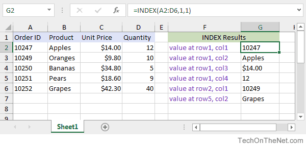
Based on the Excel spreadsheet above, the following INDEX examples would return:

=INDEX(A2:D6,1,1)
Result: 10247     'Intersection of row1 and col1 (cell A2)

=INDEX(A2:D6,1,2)
Result: "Apples"  'Intersection of row1 and col2 (cell B2)

=INDEX(A2:D6,1,3)
Result: $14.00    'Intersection of row1 and col3 (cell C2)

=INDEX(A2:D6,1,4)
Result: 12        'Intersection of row1 and col4 (cell D2)

=INDEX(A2:D6,2,1)
Result: 10249     'Intersection of row2 and col1 (cell A3)

=INDEX(A2:D6,5,2)
Result: Grapes    'Intersection of row5 and col2 (cell B6)

Now, let’s look at the example =INDEX(A2:D6,1,1) that returns a value of 10247 and take a closer look why.

First Parameter

The first parameter in the INDEX function is the table or the source of data where the lookup should be performed.

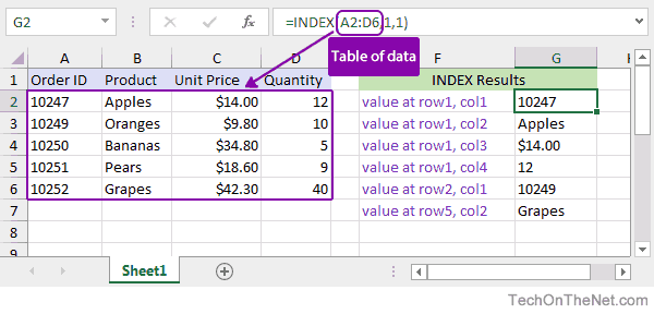
In this example, the first parameter is A2:D6 which defines the range of cells that contains the data.

Second Parameter

The second parameter is the row number used to determine the intersection location in the table. A value of 1 indicates the first row in the table, a value of 2 is the second row, and so on.

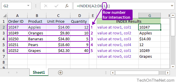
In this example, the second parameter is 1 so we know that our intersection will occur in the first row in the table.

Third Parameter

The third parameter is the column number used to determine the intersection location in the table. A value of 1 indicates the first column in the table, a value of 2 is the second column, and so on.

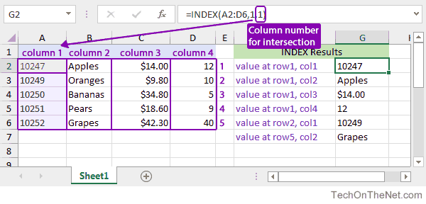
In this example, the third parameter is 1 so we know that our intersection will occur in the first column in the table.

Since we now have our row and column values, we know that we are looking for the intersection of row1 and col1 in the table of data. This makes the intersection point occur at cell A2 in the table so the INDEX function will return the value 10247.

Frequently Asked Questions

If you want to find out what others have asked about the INDEX function, go to our Frequently Asked Questions.

Frequently Asked Questions

Источник

The INDEX function in Excel helps extract the value of a cell, which is within a specified array (range) and, at the intersection of the stated row and column numbers. In other words, the function goes to the cell (within a particular range) whose position is specified, picks its value, and returns it as the output. The INDEX function can also extract an array of values from a dataset.

For example, a worksheet contains the names of continents and the corresponding countries. The entries, typed in Excel (without the double quotation marks), are listed as follows:

Column A

Cell A1 contains “Asia.”
Cell A2 contains “Africa.”
Cell A3 contains “Europe.”
Cell A4 contains “North America.”

Column B

Cell B1 contains “India.”
Cell B2 contains “Nigeria.”
Cell B3 contains “France.”
Cell B4 contains “Canada.”

Enter the formula “=INDEX(A1:B4,3,2)” in cell C1. Press the “Enter” key and the output is “France” (without the double quotation marks).

First, the INDEX excel function goes to the range A1:B4. From this range, it fetches the value of the cell, which is at the intersection of the third row (row 3) and the second column (column B). This cell is B3 and its value is “France.”

The INDEX function can return the following values:

The value at the intersection of the specified row and column numbers
The value within a table or a named range whose row and column numbers are specified
The value within non-adjacent ranges whose row and column numbers are specified

The INDEX function in Excel is useful when the dataset is large and one knows the position of the cell from which the value needs to be extracted.

The INDEX function is categorized under the Lookup and Reference functions of Excel.

You are free to use this image on your website, templates, etc, Please provide us with an attribution linkArticle Link to be Hyperlinked
For eg:
Source: INDEX Function in Excel (wallstreetmojo.com)

Index Function in Excel
- Syntax of the INDEX Function in Excel
- How to use the INDEX Function in Excel?
  - Example #1–Array Form With a One-Dimensional Array
  - Example #2–Array Form With a Two-Dimensional Array
  - Example #3–Array Form With Row and/or Column Numbers as Zeros
  - Example #4–Reference Form With Multiple Two-Dimensional Arrays
- The Properties Applicable to Both Forms of the INDEX Function
- The INDEX With Other Functions of Excel
- Frequently Asked Questions
- Recommended Articles

Syntax of the INDEX Function in Excel

There are two forms of the INDEX function in excel, the array and the reference. The syntax of both forms is shown in the following image.

Let us discuss both forms of the Excel INDEX function one by one.

The Array Form of the INDEX Excel Function

In the array form, the INDEX function fetches the value of a cell within an array or a table. An array can be either a single range of cells (horizontal or vertical) or multiple adjacent ranges. The value of the cell, which is at the intersection of the supplied row and column numbers, is returned.

The INDEX function accepts the following arguments in the array form:

Array: This can be a range of cells, table, array constant or named rangeName range in Excel is a name given to a range for the future reference. To name a range, first select the range of data and then insert a table to the range, then put a name to the range from the name box on the left-hand side of the window.read more. The cell whose value is to be returned must necessarily be within this array.
Row_num: This is the row number of the array from which the value is to be returned.
Column_num: This is the column number of the array from which the value is to be returned.

The arguments “array” and “row_num” are mandatory, while the argument “column_num” is optional.

It is essential to specify either the “row_num” or the “column_num” to extract a value from a one-dimensional array. To extract a value from a two-dimensional array, one needs to specify both, the “row_num” and the “column_num.”

Note 1: A one-dimensional array consists of a single row or a single column. A two-dimensional array consists of multiple rows and columns.

Note 2: If both “row_num” and “column_num” are entered as zeros (or blanks), the “#VALUE!” error is returned. For instance, the formulas “=INDEX(A1:A4,0,0)” and “=INDEX(A1:A4,,)” return the “#VALUE!” error.

Note 3: If the “array” argument consists of a single column, the “column_num” argument can be omitted, but the “row_num” must be supplied to fetch the value. Likewise, if the “array” argument consists of a single row, the “row_num” argument can be omitted, but the “column_num” must be specified to fetch the value.

For instance, in case of a single column, use the formula “=INDEX(array,row_num)” to fetch a value. In case of a single row, use the formula “=INDEX(array,,column_num)” to fetch a value.

The Reference Form of the INDEX Excel Function

In the reference form, the INDEX function fetches the value of a cell within a defined area (array or range). There can be multiple non-adjacent areas in the reference form. In such cases, the particular area, within which the INDEX function should look for the value, can be specified.

The INDEX function in Excel accepts the following arguments in the reference form:

Reference: This is the area which can either be a single range or multiple non-adjacent ranges. In the case of multiple non-adjacent ranges, use commas to separate the ranges. In addition, all the ranges must be enclosed within parentheses. For instance, the “reference” argument, (A1:C2, C4:D7) implies two areas (arrays or ranges), A1:C2 and C4:D7.
Row_num: This is the row number of the area from which the value is to be returned.
Column_num: This is the column number of the area from which the value is to be returned.
Area_num: This number indicates the area (of the “reference” argument) in which the INDEX function will look for a value. The first area of the “reference” argument is assigned the number 1. The second area is numbered 2 and so on. For instance, if the “reference” argument is (A1:C2, C4:D7, F4:H8) and the “area_num” is 3, the INDEX function looks for the value in the third area of the “reference” argument, i.e., F4:H8.

The arguments “reference” and “row_num” are required, while the arguments “column_num” and “area_num” are optional.

In the following image, the grey box (pointed by the red arrow) shows the different areas (arrays or ranges) of the reference argument. Further, the area numbers of each range are also given.

Note 1: If the “area_num” argument is omitted, the INDEX excel function looks for the value in the first area of the “reference” argument.

Note 2: All the areas stated in the “reference” argument should be located on one worksheet. If the first area is in one worksheet and the second is in another, the INDEX function returns the “#VALUE!” error.

Note 3: The difference between the array and reference forms is that in the former, adjacent ranges are used, while in the latter, non-adjacent ranges are used.

How to use the INDEX Function in Excel?

Let us consider a few examples to understand the working of the INDEX function in Excel.

You can download this INDEX Function Excel Template here – INDEX Function Excel Template

Example #1–Array Form With a One-Dimensional Array

The following image shows the number of employees (column C) working in the different departments (column B) of an organization.

We want to extract the value of cell C7 with the help of the INDEX function. Use the array form with column C as the single array.

The steps to perform the given task are listed as follows:

Step 1: Enter the following formula in cell E2.

“=INDEX(C3:C7,5)”

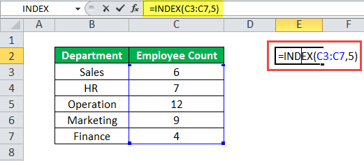
Step 2: Press the “Enter” key. The output in cell E2 is 4.

Explanation: In the formula entered in step 1, we omitted the “column_num” argument since the array (C3:C7) is a single column. Cell C7 is in the fifth row of the array C3:C7. So, the “row_num” argument is entered as 5.

Hence, the given INDEX formula returns 4, which is the value of row 5 of the range C3:C7.

Example #2–Array Form With a Two-Dimensional Array

The following image shows the total number of employees working in five departments of a multinational corporationA multinational company (MNC) is defined as a business entity that operates in its country of origin and also has a branch abroad. The headquarter usually remains in one country, controlling and coordinating all the international branches.
read more (MNC). The numbers pertain to four years, namely, 2015-2018.

We want to extract the value of cell E5 with the help of the INDEX excel function. Use the array form with the entire dataset (except the headings in row 2) as the array.

The steps to perform the given task are listed as follows:

Step 1: Enter the following formula in cell B9.

“=INDEX(B3:F7,3,4)”

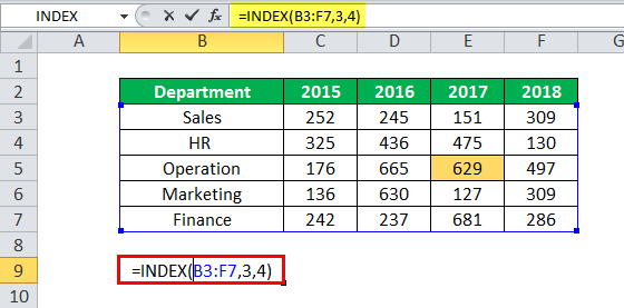
Step 2: Press the “Enter” key. The output in cell B9 is 629.

Explanation: In the preceding formula (entered in step 1), the multiple rows and columns of the dataset are entered as a single array (B3:F7). The INDEX formula returns the value of the cell, which is at the intersection of row 3 and column 4 of the range B3:F7. The cell at this position is cell E5 and its value is 629.

Hence, the output, 629, corresponds to the third row and fourth column of the range B3:F7.

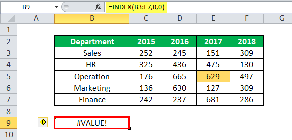
Example #3–Array Form With Row and/or Column Numbers as Zeros

Working on the data of example #2, we want to apply the INDEX function to the entire dataset (B3:F7). Further, observe the output in the following cases:

Case 1: When both arguments “row_num” and “column_num” are zeros

Case 2: When either the “row_num” or the “column_num” is zero

The two cases are discussed as follows:

Case 1: When both row and column numbers are entered as zeros, the INDEX function returns the “#VALUE” error.

Steps to be followed: Enter the formula “=INDEX(B3:F7,0,0)” in cell B9. Press the “Enter” key and the output is the “#VALUE” error. This is shown in the following image.

Conclusion: When multiple rows and columns are used as an array, it is necessary to specify both the row and column numbers to extract a particular cell value. In case, both row and column numbers are entered as zeros, the output is the “#VALUE” error.

Case 2: When either the row or the column number is zero, and the INDEX formula is entered as an array formula, the output is an array of values.

Steps to be followed: Select the blank range B11:B15. Enter the formula “=INDEX(B3:F7,0,1)” in the first cell selected (cell B11). Press the keys “Ctrl+Shift+Enter” together.

The outputs in cells B11, B12, B13, B14, and B15 are “Sales,” “HR,” “Operation,” “Marketing,” and “Finance” respectively. All outputs are obtained (without the double quotation marks) the way they are displayed in the range B3:B7.

Alternatively, select the blank row D11:H11. Enter the formula “=INDEX(B3:F7,3,0)” as an array formula. The output is the array of values of row 5 (of the preceding image). So, the output is “Operation,” “176,” “665,” “629,” and “497” without the double quotation marks.

Conclusion: When either the row or column number is specified while the other is set at zero, the INDEX function returns an array of values. However, in such cases, the INDEX formula must be entered as an array formula.

Moreover, it is essential to select a blank output range prior to entering the INDEX formula. This output range should have as many blank cells as the array of the source dataset.

Note: An array formula is usually completed by pressing the CSE keys (Ctrl+Shift+Enter).

Example #4–Reference Form With Multiple Two-Dimensional Arrays

The following image contains three datasets which display the number of employees working in the different departments of an MNC. The first dataset (B2:E7) shows the figures for the years 2015-2017. The second (D9:F12) and third datasets (C14:E18) show the figures for the years 2015 and 2016.

Use the reference form of the INDEX excel function to extract the value of cell F11. Further, categorize the three datasets into three areas which exclude the top row containing the headings.

The steps to perform the preceding tasks are listed as follows:

Step 1: Enter the following formula in cell B20.

“=INDEX((B3:E7,D10:F12,C15:E18),2,3,2)”

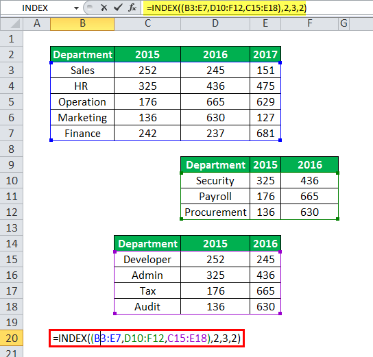
Step 2: Press the “Enter” key. The output is 665, as shown in the following image.

Explanation: In the preceding formula (entered in step 1), the three datasets (given in the question of this example) have been categorized into three areas of the “reference” argument. These areas are B3:E7, D10:F12, and C15:E18. The headings have been excluded from these areas.

Further, the INDEX function looks for a value in the second area (D10:F12). This is because the “area_num” argument is 2. The arguments “row_num” and “column_num” are 2 and 3 respectively. So, the INDEX function returns the value of the cell, which is at the intersection of the second row and the third column in the area D10:F12. This is cell F11.

Hence, the output of the INDEX formula is 665.

The Properties Applicable to Both Forms of the INDEX Function

The properties applicable to both the array and reference forms are listed as follows:

a. If both the arguments “row_num” and “column_num” are entered as zeros, the INDEX excel function returns the “#VALUE!” error.

b. To fetch a value from a single column array, use the following formulas:

“=INDEX(array,row_num)” in the array form
“=INDEX((reference),row_num,,area_num)” in the reference form

To fetch a value from a single row array, use the following formulas:

“=INDEX(array,,column_num)” in the array form
“=INDEX((reference),,col_num,area_num)” in the reference form

c. If all the column values of an array are required vertically, specify the “column_num” and set the “row_num” at zero. Likewise, if all the row values of an array are required horizontally, specify the “row_num” and set the “column_num” at zero. In both cases, select a blank output range prior to entering the INDEX formula. Moreover, press the keys “Ctrl+Shift+Enter” to complete the formula.

d. The arguments “row_num,” “column_num,” and “area_num” should refer to a cell within the defined array or reference. If not, the INDEX function returns the “#REF!” error.

Note: In pointer “c,” the blank output range can be selected vertically or horizontally depending on whether a vertical or a horizontal array is required.

Further, the number of blank cells (of the output range) must be equal to the cells of the particular row or column array (which is being copied) of the source dataset.

The INDEX With Other Functions of Excel

The INDEX function in excel can be used with several other functions of Excel in the following ways:

a. The INDEX function is used in combination with functions like SUM, AVERAGE, MIN, and MAX to create dynamic ranges. For instance, the formula “AVERAGE(C3:INDEX(C3:C7,3))” returns the average of cells C3, C4, and C5. This is because the formula “INDEX(C3:C7,3)” returns a reference to cell C5. So, the resulting formula becomes “AVERAGE(C3:C5).” Moreover, with a change in the “row_num” argument of the INDEX function, the range of the AVERAGE function changes. This results in a change in the output obtained.

b. The INDEX and MATCH The MATCH function looks for a specific value and returns its relative position in a given range of cells. The output is the first position found for the given value. Being a lookup and reference function, it works for both an exact and approximate match. For example, if the range A11:A15 consists of the numbers 2, 9, 8, 14, 32, the formula “MATCH(8,A11:A15,0)” returns 3. This is because the number 8 is at the third position.
read more functions are used together to perform left lookups. This combination of the INDEX and MATCH functions overcomes the limitations of the VLOOKUP function of Excel. For instance, limitations like compulsory sorting of data, restricted size of the lookup value, decreased speed of Excel, and so on are eliminated.

c. The INDEX function can be used with the COUNTA functionThe COUNTA function is an inbuilt statistical excel function that counts the number of non-blank cells (not empty) in a cell range or the cell reference. For example, cells A1 and A3 contain values but, cell A2 is empty. The formula “=COUNTA(A1,A2,A3)” returns 2.
read more to extract the value of the last used cell of a dataset. With a change in the value of the last used cell, the output updates on its own.

Note 1: Dynamic ranges automatically update with the addition or deletion of data.

Note 2: Usually, the INDEX function returns the value of a cell. However, when a cell referenceCell reference in excel is referring the other cells to a cell to use its values or properties. For instance, if we have data in cell A2 and want to use that in cell A1, use =A2 in cell A1, and this will copy the A2 value in A1.read more and colon (:) precede the INDEX function, it returns a cell reference. This can be observed in the AVERAGE and INDEX formula of pointer “a.”

Frequently Asked Questions

1. Define the INDEX function in Excel.

The INDEX function in Excel returns the value of a cell whose array has been defined. In addition, the row and column numbers of this cell are also specified in the arguments of the INDEX formula.

The INDEX function can also retrieve the values of the entire row or column of a range. The INDEX function has two versions, the array and the reference. Both versions have their own set of arguments.

Note: For details related to the arguments of the INDEX function, refer to the heading “the syntax of the INDEX function in Excel” of this article.

2. How to use the INDEX function in Excel?

The steps for using the INDEX function in Excel are listed as follows:

a. Select the relevant form (array or reference) of the INDEX function to be applied. For this, take into consideration the kind of data.
b. Supply the arguments to the INDEX function. If an array of values is required, select a blank output range prior to entering the arguments.
c. Press either the “Enter” key or the CSE (Ctrl+Shift+Enter) keys, depending on the kind of output required.

The INDEX function processes the arguments. Next, it returns either a single value or an array of values based on the way it has been used.

3. How to use the INDEX MATCH function in place of the VLOOKUP function in Excel?

The INDEX MATCH functions are a versatile combination. This is because these functions can easily lookup a value, regardless of the location of the lookup and the return columns.

The formula to perform a lookup (in rows and columns) by using the INDEX MATCH functions is stated as follows:

“=INDEX(column to return a value from,MATCH(vlookup value,column to be looked up,0),MATCH(hlookup value,row to be looked up,0))”

The working of this formula is explained as follows:

a. The formula “MATCH(vlookup value,column to be looked up,0)” looks for the vlookup value in the column to be looked up (or lookup column). This formula looks for the exact match and returns the row number.
b. The formula “MATCH(hlookup value,row to be looked up,0)” looks for the hlookup value in the row to be looked up (or lookup row). This formula looks for the exact match and returns the column number.
c. The INDEX function uses the row and column numbers returned by the MATCH function. The INDEX function returns a corresponding value from the “column to return a value from” (or return column).

Hence, the INDEX and MATCH formula returns a value at the intersection of certain row and column numbers.

Note 1: It is also possible to supply only the row number or only the column number to the INDEX function. For supplying only the row number, use the first MATCH formula (given in pointer “a”) with the INDEX function. Likewise, to supply only the column number, use the second MATCH formula (given in pointer “b”) with the INDEX function.

Note 2: Looking for a value at the intersection of a row and column is called a 2-way lookup (or 2-dimensional lookup or matrix lookup).

The two forms of INDEX function

The index function comes in two forms, one is called the Array form and the other is called the Reference form.

Excel displays the syntax of both forms as soon as you type the function name with an opening bracket.

I’ll try and explain both versions in simple terms. I’ll begin with the first one which is the Array form.

It is worth noting that the array version of this function is used more often than the reference version, and hence you are also more likely to use it.

INDEX function syntax (Array Form)

As I mentioned before, let’s understand how the array form of the function works before we look at the reference form. Below is the syntax breakdown of the Index function.

Syntax: INDEX(array, row_num, [column_num])

This function has three arguments: array, row_num, and [column_num].

Before we get our hands on an example, let’s quickly address these arguments one after the other. Knowing what a function argument does mean you are just halfway to mastering it.

So, below are the three arguments explained in simple terms.

array: This represents a range of cells that has the data. This range could be a table or just an ordinary grid of cells. When specifying this range, make sure it covers all the rows and columns that contain your data.
row_num: This represents a row number in a range. This row number is not referring to the row number in the actual worksheet. Rather, it is the relative row position in the table (range). This row number must not exceed the total number of rows in the table. When that happens, you’ll get a #REF! as a result which is Excel’s way of telling you that the cell you are referring to does not exist.
[column_num]: This represents a column number in a range. This argument refers to the relative column position in the table (range) and not the actual worksheet column number. The column number must not be greater than the total number of columns in the table or else you’ll get #REF! as a result.

What this function return

What this function return is a value found in the intersection cell of the row and column position specified.

Now let’s see how the INDEX function works in the following example.

INDEX Function Example 1 (Array form)

Using the sample table above, let’s illustrate how the index function works. Assuming the above table is sorted in an order that the first name in the list is our first customer, the second name is our second customer, then in that order up to the end.

Using the index function on this worksheet, we’ll find and retrieve the product our 5^th customer bought. In other words, the 5^th row in the 3^rd column (or the intersection of row 5 and column 3).

The function to perform this task is shown below:

=INDEX(B5:B14,5,3)

How to write the INDEX function

First of all, type the equal sign followed by the word INDEX.

When you begin typing the function with the first two letters IN, Excel will show you all the functions that begin with these letters.

Fortunately, the first suggested function is the INDEX function. So, there’s no need to finish typing it. Just press the tab key and excel will gladly insert the function for you.

However, if you use the tab key to auto-complete the function name, Excel will insert the opening bracket for you. Just make sure that you don’t forget and type another opening bracket.

Index function 1^st argument (array)

=INDEX(B5:B14,

Now, let’s specify the first argument of this function, which is the array argument.

This argument indicates the range of cells we are interested in. According to our sample table, the data covers cell B5:B14. We will, therefore, use this range as the first argument (array).

You can also use a named range for this argument, like CustomerTable or SalesTable.

To assign a name to any range of cells, highlight the range and go to the Name Box, type the name you wish to assign to the range, then press enter to apply the name.

You can, therefore, specify the array argument with this name.

See screenshot:

Index function 2^nd argument (row_num)

=INDEX(B5:B14,5

A value of 1 indicates the first row in the table (or range), a value of 2 indicates the second row in the table (or range), and in that order.

The second argument finds the row we want, and that is the 5^th row. Obviously, this argument will be 5 since we are referring to the 5^th row.

See screenshot:

Here, the function is not spotting the row based on any specific data as in VLOOKUP. Rather, the function is spotting the 5^th row because we specified 5 as the row number.

After specifying an argument, don’t forget to bring a comma sign before typing the next argument.

Index function 3^rd argument ([column_num])

=INDEX(B5:B14,5,3)

The third argument represents the index number of the product column which is 3. A value of 1 and 2 indicate the first and second columns in the table. The value of 3, therefore, means that you are referring to the third column in the table.

After providing all the arguments, close the brackets and press Enter key to see the result.

Result

When you enter the formula, the result says Product B. This is supposed to be the value of the cell in the 5^th row of the 3^rd column, which is cell D9. In other words, the intersection cell of row 5 and column 3.

More INDEX Function Examples

With this data, try your hands on more examples of the INDEX function to gain some experience. You can download the example file below and practice with it.

The main reason I brought these formulas is for you to see the different ways you can refer to ranges when dealing with the INDEX function.

See the second row, for instance, I only specify the array and the row number. I still got a result even though I didn’t specify the column number. This is because the range is one-dimensional, meaning it has only one column. Even if you don’t bring the column number, excel can still work with that since it got no options to choose from.

Now let’s look at the other version of the INDEX – Reference form.

Index function syntax (Reference Form)

The array form of the INDEX function has been explained in considerable detail.

Now let’s focus our attention on the other form of the function – the reference form.

Syntax: INDEX(reference, row_num, [column_num], [area-num])

One thing you should take note of is the key difference between the two forms which lies in the choice of arguments for the function. While the Array form of the INDEX works with a single table, the reference form can work with multiple tables. Therefore, you don’t need to use the Reference form of the INDEX function if you are referring to only one table in the formula.

Let’s get familiar with the arguments of this form of INDEX.

reference: This represents a reference to one or more cell ranges.
Row_num: This argument specifies the number of a row in a reference (or range of cells). If each range in the reference contains only one row, the row_num argument is optional.
[Column_num]: Specifies the number of a column in a reference (or range of cells). If each range in the reference contains only one column, then the column_num argument is optional.
[area_num]: This argument specifies one of the ranges in reference from which to return the intersection cell of a specified row and column. Since the Reference form of the INDEX function works with multiple tables, the [area_num] argument is used to select the table to use. 1 is used to select the first area (or table/range), 2 for the second area (or table/range), and so on.

INDEX() function example 2 (Reference form)

The above picture shows two tables with different data. Our goal here is to use both of these tables as references inside the INDEX function.

Therefore, imagine you want to write a formula that will refer to these two tables and retrieve a value from the second table.

Let’s take, for example, the quantity for Daniel is in table two. Daniel is in the 7^th row (excluding the header row) whilst quantity is in the 4^th column. We then need the formula to retrieve the intersection cell of row 7 and column 4.

Below is the formula:

=INDEX((B6:E15,G6:J15),7,4,2)

INDEX Formula breakdown

I mentioned before that the main difference between the Array form and Reference form of the INDEX function lies in the arguments. If you have only one table to deal with, go with the array form, otherwise, the reference form is what you need.

Here’s the case we have two tables and want to include both in the INDEX formula. Let’s see how you can do that.

1^st argument: Reference

This argument is what differentiates between the two forms of INDEX. In the reference version, this argument can refer to more than one table.

To refer to more ranges (or tables) than one, surround the ranges with parenthesis and separate them with a comma.

See screenshot:

2^nd and 3^rd arguments

The 2^nd and 3^rd arguments determine the row and column numbers respectively. These arguments, in particular, don’t change at all as compared to the Array form of the INDEX function. The 7 and 4 specify the row and column numbers respectively. The new thing here is the last argument – [area_num].

Final argument: [area_num]

What the area number argument does is very simple. It specifies which range in the reference to use. Since we are referring to multiple tables in the reference, we need to specify the table we want to work with. An argument of 1 will refer to the first table, an argument of 2 to the second table, and so on.

Bonus tips

Writing formulas that include values or text is not a good practice at all. If an argument requires a value or a text, whenever you wish to change this argument, you’ll be forced to crack open the formula for editing.

This is not a problem when you have only one or a few formulas on the line. It only becomes a big problem when you are working with countless formulas.

To avoid these problems in your formulas, always try and avoid using values and use cell references instead.

In other words, if your formula is going to need an argument that is a value (say 2), don’t write the value (2) into the formula. Instead, write the value (2) into another cell and then refer to that cell in the formula. This way, whenever you want to change this particular argument to 4, all you need to do is change the value in that cell.

Let’s try this idea with the first example we worked on.

See screenshot:

As seen in the above example, instead of using 5 for the row number argument and 2 for the column number argument, the formula referred to cells C2 and C3 which contain the values to be used for the arguments.

Assuming you want to change the row number or column number, you don’t have to edit the formula to do so. Changing the content in Cells C2 and C3 is all it’ll take.

See screenshot:

As seen in the above example, as you edit the content in cells C2 and C3, the result for the INDEX function also changes.

Источник

Функция INDEX (ИНДЕКС) в Excel используется для получения данных из таблицы, при условии что вы знаете номер строки и столбца, в котором эти данные находятся.

Например, в таблице ниже, вы можете использовать эту функцию для того, чтобы получить результаты экзамена по Физике у Андрея, зная номер строки и столбца, в которых эти данные находятся.

Содержание

Что возвращает функция
Синтаксис
Аргументы функции
Дополнительная информация
Примеры использования функции ИНДЕКС в Excel
Пример 1. Ищем результаты экзамена по физике для Алексея
Пример 2. Создаем динамический поиск значений с использованием функций ИНДЕКС и ПОИСКПОЗ
Пример 3. Создаем динамический поиск значений с использованием функций INDEX (ИНДЕКС) и MATCH (ПОИСКПОЗ) и выпадающего списка
Пример 4. Использование трехстороннего поиска с помощью INDEX (ИНДЕКС) / MATCH (ПОИСКПОЗ)

Что возвращает функция

Возвращает данные из конкретной строки и столбца табличных данных.

Синтаксис

=INDEX (array, row_num, [col_num]) — английская версия

=INDEX (array, row_num, [col_num], [area_num]) — английская версия

=ИНДЕКС(массив; номер_строки; [номер_столбца]) — русская версия

=ИНДЕКС(ссылка; номер_строки; [номер_столбца]; [номер_области]) — русская версия

Аргументы функции

array (массив) — диапазон ячеек или массив данных для поиска;
row_num (номер_строки) — номер строки, в которой находятся искомые данные;
[col_num] ([номер_столбца]) (необязательный аргумент) — номер колонки, в которой находятся искомые данные. Этот аргумент необязательный. Но если в аргументах функции не указаны критерии для row_num (номер_строки), необходимо указать аргумент col_num (номер_столбца);
[area_num] ([номер_области]) — (необязательный аргумент) — если аргумент массива состоит из нескольких диапазонов, то это число будет использоваться для выбора всех диапазонов.

Дополнительная информация

Если номер строки или колонки равен “0”, то функция возвращает данные всей строки или колонки;
Если функция используется перед ссылкой на ячейку (например, A1), она возвращает ссылку на ячейку вместо значения (см. примеры ниже);
Чаще всего INDEX (ИНДЕКС) используется совместно с функцией MATCH (ПОИСКПОЗ);
В отличие от функции VLOOKUP (ВПР), функция INDEX (ИНДЕКС) может возвращать данные как справа от искомого значения, так и слева;
Функция используется в двух формах — Массива данных и Формы ссылки на данные:

— Форма «Массива» используется когда вы хотите найти значения, основанные на конкретных номерах строк и столбцов таблицы;

— Форма «Ссылок на данные» используется при поиске значений в нескольких таблицах (используете аргумент [area_num] ([номер_области]) для выбора таблицы и только потом сориентируете функцию по номеру строки и столбца.

Примеры использования функции ИНДЕКС в Excel

Пример 1. Ищем результаты экзамена по физике для Алексея

Предположим, у вас есть результаты экзаменов в табличном виде по нескольким студентам:

Для того, чтобы найти результаты экзамена по физике для Андрея нам нужна формула:

=INDEX($B$3:$E$9,3,2) — английская версия

=ИНДЕКС($B$3:$E$9;3;2) — русская версия

В формуле мы определили аргумент диапазона данных, где мы будем искать данные $B$3:$E$9. Затем, указали номер строки “3”, в которой находятся результаты экзамена для Андрея, и номер колонки “2”, где находятся результаты экзамена именно по физике.

Пример 2. Создаем динамический поиск значений с использованием функций ИНДЕКС и ПОИСКПОЗ

Не всегда есть возможность указать номера строки и столбца вручную. У вас может быть огромная таблица данных, отображение данных которой вы можете сделать динамическим, чтобы функция автоматически идентифицировала имя или экзамен, указанные в ячейках, и дала правильный результат.

Пример динамического отображения данных ниже:

Для динамического отображения данных мы используем комбинацию функций INDEX (ИНДЕКС) и MATCH (ПОИСКПОЗ).

Вот такая формула поможет нам добиться результата:

=INDEX($B$3:$E$9,MATCH($G$4,$A$3:$A$9,0),MATCH($H$3,$B$2:$E$2,0)) — английская версия

=ИНДЕКС($B$3:$E$9;ПОИСКПОЗ($G$4;$A$3:$A$9;0);ПОИСКПОЗ($H$3;$B$2:$E$2;0)) — русская версия

В формуле выше, не используя сложного программирования, мы с помощью функции MATCH (ПОИСКПОЗ) сделали отображение данных динамическим.

Динамический отображение строки задается следующей частью формулы —

MATCH($G$4,$A$3:$A$9,0) — английская версия

ПОИСКПОЗ($G$4;$A$3:$A$9;0) — русская версия

Она сканирует имена студентов и определяет значение поиска ($G$4 в нашем случае). Затем она возвращает номер строки для поиска в наборе данных. Например, если значение поиска равно Алексей, функция вернет “1”, если это Максим, оно вернет “4” и так далее.

Динамическое отображение данных столбца задается следующей частью формулы —

MATCH($H$3,$B$2:$E$2,0) — английская версия

ПОИСКПОЗ($H$3;$B$2:$E$2;0) — русская версия

Она сканирует имена объектов и определяет значение поиска ($H$3 в нашем случае). Затем она возвращает номер столбца для поиска в наборе данных. Например, если значение поиска Математика, функция вернет “1”, если это Физика, функция вернет “2” и так далее.

Больше лайфхаков в нашем Telegram Подписаться

Пример 3. Создаем динамический поиск значений с использованием функций INDEX (ИНДЕКС) и MATCH (ПОИСКПОЗ) и выпадающего списка

На примере выше мы вручную вводили имена студентов и названия предметов. Вы можете сэкономить время на вводе данных, используя выпадающие списки. Это актуально, когда количество данных огромное.

Используя выпадающие списки, вам нужно просто выбрать из списка имя студента и функция автоматически найдет и подставит необходимые данные.

Пример ниже:

Используя такой подход, вы можете создать удобный дашборд, например для учителя. Ему не придется заниматься фильтрацией данных или прокруткой листа со студентами, для того чтобы найти результаты экзамена конкретного студента, достаточно просто выбрать имя и результаты динамически отразятся в лаконичной и удобной форме.

Для того, чтобы осуществить динамическую подстановку данных с использованием функций INDEX (ИНДЕКС) и MATCH (ПОИСКПОЗ) и выпадающего списка, мы используем ту же формулу, что в Примере 2:

=INDEX($B$3:$E$9,MATCH($G$4,$A$3:$A$9,0),MATCH($H$3,$B$2:$E$2,0)) — английская версия

=ИНДЕКС($B$3:$E$9;ПОИСКПОЗ($G$4;$A$3:$A$9;0);ПОИСКПОЗ($H$3;$B$2:$E$2;0)) — русская версия

Единственное отличие, от Примера 2, мы на месте ввода имени и предмета создадим выпадающие списки:

Выбираем ячейку, в которой мы хотим отобразить выпадающий список с именами студентов;
Кликаем на вкладку “Data” => Data Tools => Data Validation;
В окне Data Validation на вкладке “Settings” в подразделе Allow выбираем “List”;
В качестве Source нам нужно выбрать диапазон ячеек, в котором указаны имена студентов;
Кликаем ОК

Теперь у вас есть выпадающий список с именами студентов в ячейке G5. Таким же образом вы можете создать выпадающий список с предметами.

Пример 4. Использование трехстороннего поиска с помощью INDEX (ИНДЕКС) / MATCH (ПОИСКПОЗ)

Функция INDEX (ИНДЕКС) может быть использована для обработки трехсторонних запросов.

Что такое трехсторонний поиск?

В приведенных выше примерах мы использовали одну таблицу с оценками для студентов по разным предметам. Это пример двунаправленного поиска, поскольку мы используем две переменные для получения оценки (имя студента и предмет).

Теперь предположим, что к концу года студент прошел три уровня экзаменов: «Вступительный», «Полугодовой» и «Итоговый экзамен».

Трехсторонний поиск — это возможность получить отметки студента по заданному предмету с указанным уровнем экзамена.

Вот пример трехстороннего поиска:

В приведенном выше примере, кроме выбора имени студента и названия предмета, вы также можете выбрать уровень экзамена. Основываясь на уровне экзамена, формула возвращает соответствующее значение из одной из трех таблиц.

Для таких расчетов нам поможет формула:

=INDEX(($B$3:$E$7,$B$11:$E$15,$B$19:$E$23),MATCH($G$4,$A$3:$A$7,0),MATCH($H$3,$B$2:$E$2,0),IF($H$2=»Вступительный»,1,IF($H$2=»Полугодовой»,2,3))) — английская версия

=ИНДЕКС(($B$3:$E$7;$B$11:$E$15;$B$19:$E$23);ПОИСКПОЗ($G$4;$A$3:$A$7;0);ПОИСКПОЗ($H$3;$B$2:$E$2;0); ЕСЛИ($H$2=»Вступительный»;1;ЕСЛИ($H$2=»Полугодовой»;2;3))) — русская версия

Давайте разберем эту формулу, чтобы понять, как она работает.

Эта формула принимает четыре аргумента. Функция INDEX (ИНДЕКС) — одна из тех функций в Excel, которая имеет более одного синтаксиса.

=INDEX (array, row_num, [col_num]) — английская версия

=INDEX (array, row_num, [col_num], [area_num]) — английская версия

=ИНДЕКС(массив; номер_строки; [номер_столбца]) — русская версия

=ИНДЕКС(ссылка; номер_строки; [номер_столбца]; [номер_области]) — русская версия

По всем вышеприведенным примерам мы использовали первый синтаксис, но для трехстороннего поиска нам нужно использовать второй синтаксис.

Рассмотрим каждую часть формулы на основе второго синтаксиса.

array (массив) – ($B$3:$E$7,$B$11:$E$15,$B$19:$E$23):Вместо использования одного массива, в данном случае мы использовали три массива в круглых скобках.
row_num (номер_строки) – MATCH($G$4,$A$3:$A$7,0): функция MATCH (ПОИСКПОЗ) используется для поиска имени студента для ячейки $G$4 из списка всех студентов.
col_num (номер_столбца) – MATCH($H$3,$B$2:$E$2,0): функция MATCH (ПОИСКПОЗ) используется для поиска названия предмета для ячейки $H$3 из списка всех предметов.
[area_num] ([номер_области]) – IF($H$2=”Вступительный”,1,IF($H$2=”Полугодовой”,2,3)): Значение номера области сообщает функции INDEX (ИНДЕКС), какой массив с данными выбрать. В этом примере у нас есть три массива в первом аргументе. Если вы выберете «Вступительный» из раскрывающегося меню, функция IF (ЕСЛИ) вернет значение “1”, а функция INDEX (ИНДЕКС) выберут 1-й массив из трех массивов ($B$3:$E$7).

Уверен, что теперь вы подробно изучили работу функции INDEX (ИНДЕКС) в Excel!

Источник

How to Use the INDEX Function in Excel – With Examples (2023)

INDEX function belongs to the family of LOOKUP and is an awesome function at its base.

Its primary purpose is to return a cell reference from a specified array.

But the other LOOKUP functions do the same thing, no? So what distinguishes INDEX from other functions, and how do you use it? 🤔

Read on to find answers to these and a lot more questions. This guide has all you need to know.

If you want to practice the INDEX function in real time, download our sample workbook here.

How to use INDEX – reference style

The Excel INDEX function has two versions of its syntax. These are referred to as the array form and the reference form.

Let’s first discuss the reference argument of the formula.

Its syntax is:

=INDEX(reference, =INDEX(reference, row_num, [columm_num], [area_num])

reference argument refers to the range or ranges you select – you can select more than one range. If you have multiple ranges, separate them using a comma like (A1:C4, D1:F4)
row_num parameter specifies the row number from where you want to extract the result.
column_num parameter specifies the column number containing the value to be extracted.
area_num is an optional argument. It is only used when you insert two or more ranges in the reference parameter. It specifies a particular range from the two.

Now that we are well-equipped with its syntax, let’s see how it works on actual data 🤓

We have the following example data set.

It contains the names of some students and their marks in three subjects. We want to find the total marks of Daniel B. given in cell E7.

So to do that:

Select a cell.
Enter the formula as:

=INDEX(

Add the reference as:

=INDEX(A1:E10

This specifies the range INDEX will look up for our value.

Add the next argument as:

=INDEX(A1:E10, 7, 4)

The two recent arguments specify the row and column numbers where the lookup value exists. INDEX will search the entire row and entire column for the value.

Since we only had one range, we didn’t use the area_num parameter.

Press Enter.

The Excel INDEX function returns the value 59, which is exactly what we want.

This might seem petty but wait till you use the INDEX function with large data. Your mind will be blown away 🤯

How to use INDEX – matrix style

We’ve seen how the INDEX reference style works. Let’s now explore and learn more about its array version below.

The syntax of the array form is given as follows:

=INDEX(array, row_num, [column_num])

The parameter array refers to the range of cells where we want to find our lookup value.
The row-num argument is the row number in the array where the lookup value exists.
The column-num argument specifies the column containing the lookup value.

These arguments are similar to the ones used in the reference form. And the results are also pretty identical.

Let’s test the array form on a real data set.

We have the following sample data.

And we want to find the sales percentage of iPhone 11.

To do that:

Select a cell.
Enter the INDEX formulas as:

=INDEX(

Select the array.

=INDEX(A1:C10,

Add the row and column numbers and close the brackets.

=INDEX(A1:C10, 8, 3)

Press Enter.

INDEX formula returns your result as:

Other INDEX formula examples

Let’s see some examples of the INDEX formula with other functions 😃

INDEX formula example #1

We will combine the INDEX and MATCH functions – the most commonly used duo. So let’s get started.

We have the following data set.

It contains information about the employees of a company. It shows their departments, salaries, joining years, and leaves.

We need to check the number of leaves of Alex J. using the INDEX and MATCH Formula.

To do that:

Select a cell.
Enter the formula as:

= INDEX(

Enter the reference containing the lookup value to be returned.

= INDEX(E1:E10

Combine it with the MATCH function.

= INDEX(E1:E10, MATCH(

Now, we need to add the arguments of the MATCH function. The first argument is the reference against which it will find the lookup value.

Enter the lookup_value as:

= INDEX(E1:E10, MATCH(A6,

Reference the lookup_array as:

= INDEX(E1:E10, MATCH(A6, A1:A10,

Enter the match_type – we used 0 for the exact value.

= INDEX(E1:E10, MATCH(A6, A1:A10, 0

Add the closing brackets.

The final formula looks like this:

= INDEX(E1:E10, MATCH(A6, A1:A10, 0))

Press Enter.

And voila! The MATCH function returns the leaves number of Alex J. as:

You’ve done quite some work today 🥇

INDEX formula example #2

Let’s try an easy INDEX example for this one.

Say we have the following data set that shows the total sales of some T-shirts.

We will combine the INDEX function with the MAX function to find the highest sales made in this range.

To do that:

Select a cell.
Enter the formula as:

= MAX(

Now add the INDEX function as a parameter of the MAX function.

= MAX(INDEX(

Insert the reference as:

= MAX(INDEX(A1:C10,

We will leave out the row-num argument because we want INDEX to find the highest value in the third column.

Add the column number and close the brackets.

The final formula looks like this:

= MAX(INDEX(A1:C10, , 3))

Press Enter

And INDEX returns the result as:

Pretty easy, no? 👀

This might seem a little uncalled for. But the INDEX function can be really resourceful when combined with other intricate functions for data crunching and analysis.

That’s it – What now?

Wow, we’ve learned a lot today 😅

We saw what the Excel INDEX function is and how it works. We also saw its two versions and some important INDEX examples with other functions.

It’s a really fantastic function – you just need to know when and where to use it. Luckily, Excel has a huge variety of functions similar to and more powerful than the INDEX function.

Some of these include the VLOOKUP, IF, and SUMIF functions, but there’s more to it.

You can learn these incredible functions and more for free in my 30-minute email course. It’s delivered right to your inbox only at the cost of your email address. So join now! 😃

Frequently asked questions

To know what INDEX does in Excel, you first need to know how it works. The INDEX function is an array formula. It lookups up a value in a range as we specify its row and column. INDEX returns the value given at the intersection of the specified row and column.

Kasper Langmann2023-01-21T19:57:37+00:00

Page load link

Источник

Get the value at a given position in a range or array

What is the INDEX Function?

The INDEX Function[1] is categorized under Excel Lookup and Reference functions. The function will return the value at a given position in a range or array. The INDEX function is often used with the MATCH function. We can say it is an alternative way to do VLOOKUP.

As a financial analyst, INDEX can be used in other forms of analysis besides looking up a value in a list or table. In financial analysis, we can use it along with other functions, for lookup and to return the sum of a column.

There are two formats for the INDEX function:

Array format
Reference format

The Array Format of the INDEX Function

The array format is used when we wish to return the value of a specified cell or array of cells.

Formula

=INDEX(array, row_num, [col_num])

The function uses the following arguments:

Array (required argument) – This is the specified array or range of cells.
Row_num (required argument) – Denotes the row number of the specified array. When the argument is set to zero or blank, it will default to all rows in the array provided.
Col_num (optional argument) – This denotes the column number of the specified array. When this argument is set to zero or blank, it will default to all rows in the array provided.

The Reference Format of the INDEX Function

The reference format is used when we wish to return the reference of the cell at the intersection of row_num and col_num.

Formula

=INDEX(reference, row_num, [column_num], [area_num])

The function uses the following arguments:

Reference (required argument) – This is a reference to one or more cells. If we input multiple areas directly into the function, individual areas should be separated by commas and surrounded by brackets. Such as (A1:B2, C3:D4), etc.
Row_num (required argument) – Denotes the row number of a specified area. When the argument is set to zero or blank, it will default to all rows in the array provided.
Col_num (optional argument) – This denotes the column number of the specified array. When the argument is set to zero or blank, it will default to all rows in the array provided.
Area_num (optional argument) – If the reference is supplied as multiple ranges, area_num indicates which range to use. Areas are numbered by the order they are specified.

If the area_num argument is omitted, it defaults to the value 1 (i.e., the reference is taken from the first area in the supplied range).

How to Use the INDEX Function in Excel

To understand the uses of the function, let us consider a few examples:

Example 1

We are given the following data and we wish to match the location of a value.

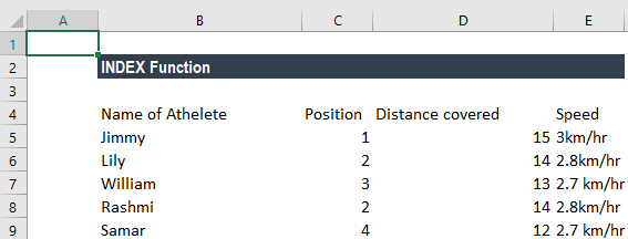
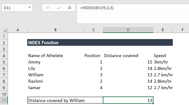
In the table above, we wish to see the distance covered by William. The formula to use will be:

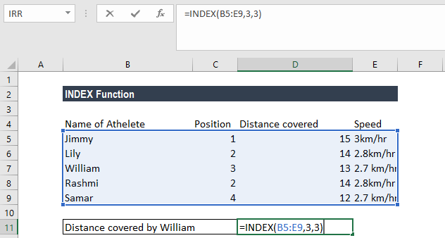
We get the result below:

Example 2

Now let’s see how to use the MATCH and INDEX functions at the same time. Suppose we are given the following data:

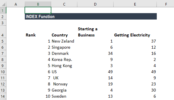
Suppose we wish to find out Georgia’s rank in the Ease of Doing Business category. We will use the following formula:

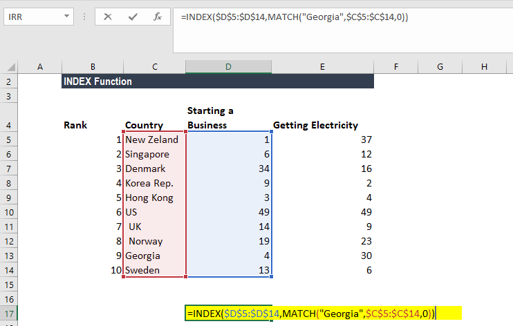
Here, the MATCH function will look up for Georgia and return number 10 as Georgia is 10 on the list. The INDEX function takes “10” in the second parameter (row_num), which indicates which row we wish to return a value from and turns into a simple =INDEX($C$2:$C$11,3).

We get the result below:

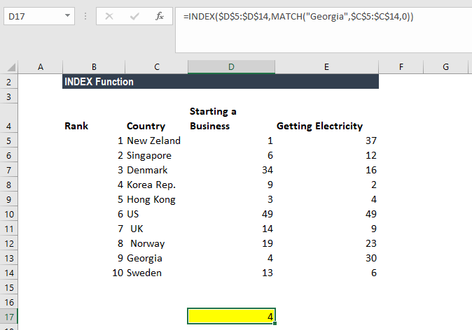
Things to Remember

#VALUE! error – Occurs when any of the given row_num, col_num or area_num arguments are non-numeric.
#REF! error – Occurs due to either of the following reasons:
- The given row_num argument is greater than the number of rows in the given range;
- The given [col_num] argument is greater than the number of columns in the range provided; or
- The given [area_num] argument is more than the number of areas in the supplied range.
VLOOKUP vs. INDEX function
- Excel VLOOKUP is unable to look to its left, meaning that our lookup value should always reside in the left-most column of the lookup range. This is not the case with the INDEX and MATCH functions.
- VLOOKUP formulas get broken or return incorrect results when a new column is deleted from or added to a lookup table. With INDEX and MATCH, we can delete or insert new columns in a lookup table without distorting the results.

Click here to download the sample Excel file

Additional Resources

Thank you for reading CFI’s guide to the INDEX Function. To learn more, check out these additional CFI resources:

Advanced Excel Formulas Course
Advanced Excel Formulas You Must Know
Excel Shortcuts for PC and Mac
Financial Analyst Program
See all Excel resources

Article Sources

INDEX Function

Источник

Array form

Description

Syntax

Remarks

Examples

Example 1

Example 2

Reference form

Description

Syntax

Remarks

Examples

See Also

Is INDEX better than Vlookup?

How do I INDEX an Excel spreadsheet?

Is INDEX a match?

What is the difference between INDEX and match in Excel?

What is a index sheet?

How do you calculate the index?

How do you create an index?

How do I use index function instead of VLOOKUP?

Why do we use index match in Excel?

What is VLOOKUP in Excel?

Is index match faster than Xlookup?

Does index match use less memory than Vlookup?

What is an index example?

How do you use index function in sheets?

How do I create an index link in Excel?

How do you calculate an index example?

How do I index a document?

Where is the index page of a document?

Is primary key an index?

Does index match work in Google Sheets?

Basic usage

INDEX and MATCH

INDEX and MATCH with horizontal table

Entire row / column

Reference as result

Two forms

Array form

Reference form

Description

Syntax

Parameters or Arguments

Returns

Applies To

Type of Function

Example (as Worksheet Function)

First Parameter

Second Parameter

Third Parameter

Frequently Asked Questions

Table of contents

Syntax of the INDEX Function in Excel

How to use the INDEX Function in Excel?

Example #1–Array Form With a One-Dimensional Array

Example #2–Array Form With a Two-Dimensional Array

Example #3–Array Form With Row and/or Column Numbers as Zeros

Example #4–Reference Form With Multiple Two-Dimensional Arrays

The Properties Applicable to Both Forms of the INDEX Function

The INDEX With Other Functions of Excel

Frequently Asked Questions

Recommended Articles

The two forms of INDEX function

INDEX function syntax (Array Form)

What this function return

INDEX Function Example 1 (Array form)

How to write the INDEX function

Index function 1st argument (array)

Index function 2nd argument (row_num)

Index function 3rd argument ([column_num])

Result

More INDEX Function Examples

Index function syntax (Reference Form)

INDEX() function example 2 (Reference form)

INDEX Formula breakdown

1st argument: Reference

Bonus tips

Что возвращает функция

Синтаксис

Index function 1^st argument (array)

Index function 2^nd argument (row_num)

Index function 3^rd argument ([column_num])

1^st argument: Reference