
Excel for Microsoft 365 Excel for Microsoft 365 for Mac Excel for the web Excel 2021 Excel 2021 for Mac Excel 2019 Excel 2019 for Mac Excel 2016 Excel 2016 for Mac Excel 2013 Excel 2010 Excel 2007 Excel for Mac 2011 Excel Starter 2010 More…Less
Tip: Try using the new XLOOKUP function, an improved version of HLOOKUP that works in any direction and returns exact matches by default, making it easier and more convenient to use than its predecessor.
This article describes the formula syntax and usage of the HLOOKUP function in Microsoft Excel.
Description
Searches for a value in the top row of a table or an array of values, and then returns a value in the same column from a row you specify in the table or array. Use HLOOKUP when your comparison values are located in a row across the top of a table of data, and you want to look down a specified number of rows. Use VLOOKUP when your comparison values are located in a column to the left of the data you want to find.
The H in HLOOKUP stands for «Horizontal.»
Syntax
HLOOKUP(lookup_value, table_array, row_index_num, [range_lookup])
The HLOOKUP function syntax has the following arguments:
-
Lookup_value Required. The value to be found in the first row of the table. Lookup_value can be a value, a reference, or a text string.
-
Table_array Required. A table of information in which data is looked up. Use a reference to a range or a range name.
-
The values in the first row of table_array can be text, numbers, or logical values.
-
If range_lookup is TRUE, the values in the first row of table_array must be placed in ascending order: …-2, -1, 0, 1, 2,… , A-Z, FALSE, TRUE; otherwise, HLOOKUP may not give the correct value. If range_lookup is FALSE, table_array does not need to be sorted.
-
Uppercase and lowercase text are equivalent.
-
Sort the values in ascending order, left to right. For more information, see Sort data in a range or table.
-
-
Row_index_num Required. The row number in table_array from which the matching value will be returned. A row_index_num of 1 returns the first row value in table_array, a row_index_num of 2 returns the second row value in table_array, and so on. If row_index_num is less than 1, HLOOKUP returns the #VALUE! error value; if row_index_num is greater than the number of rows on table_array, HLOOKUP returns the #REF! error value.
-
Range_lookup Optional. A logical value that specifies whether you want HLOOKUP to find an exact match or an approximate match. If TRUE or omitted, an approximate match is returned. In other words, if an exact match is not found, the next largest value that is less than lookup_value is returned. If FALSE, HLOOKUP will find an exact match. If one is not found, the error value #N/A is returned.
Remark
-
If HLOOKUP can’t find lookup_value, and range_lookup is TRUE, it uses the largest value that is less than lookup_value.
-
If lookup_value is smaller than the smallest value in the first row of table_array, HLOOKUP returns the #N/A error value.
-
If range_lookup is FALSE and lookup_value is text, you can use the wildcard characters, question mark (?) and asterisk (*), in lookup_value. A question mark matches any single character; an asterisk matches any sequence of characters. If you want to find an actual question mark or asterisk, type a tilde (~) before the character.
Example
Copy the example data in the following table, and paste it in cell A1 of a new Excel worksheet. For formulas to show results, select them, press F2, and then press Enter. If you need to, you can adjust the column widths to see all the data.
|
Axles |
Bearings |
Bolts |
|
4 |
4 |
9 |
|
5 |
7 |
10 |
|
6 |
8 |
11 |
|
Formula |
Description |
Result |
|
=HLOOKUP(«Axles», A1:C4, 2, TRUE) |
Looks up «Axles» in row 1, and returns the value from row 2 that’s in the same column (column A). |
4 |
|
=HLOOKUP(«Bearings», A1:C4, 3, FALSE) |
Looks up «Bearings» in row 1, and returns the value from row 3 that’s in the same column (column B). |
7 |
|
=HLOOKUP(«B», A1:C4, 3, TRUE) |
Looks up «B» in row 1, and returns the value from row 3 that’s in the same column. Because an exact match for «B» is not found, the largest value in row 1 that is less than «B» is used: «Axles,» in column A. |
5 |
|
=HLOOKUP(«Bolts», A1:C4, 4) |
Looks up «Bolts» in row 1, and returns the value from row 4 that’s in the same column (column C). |
11 |
|
=HLOOKUP(3, {1,2,3;»a»,»b»,»c»;»d»,»e»,»f»}, 2, TRUE) |
Looks up the number 3 in the three-row array constant, and returns the value from row 2 in the same (in this case, third) column. There are three rows of values in the array constant, each row separated by a semicolon (;). Because «c» is found in row 2 and in the same column as 3, «c» is returned. |
c |
Need more help?
Want more options?
Explore subscription benefits, browse training courses, learn how to secure your device, and more.
Communities help you ask and answer questions, give feedback, and hear from experts with rich knowledge.
На чтение 2 мин
Функция HLOOKUP (ГПР) в Excel используется для поиска и сопоставления данных находящихся в строках таблицы (горизонтальный поиск). Другими словами, с ее помощью вы можете искать данные из первой строки таблицы и возвращать число, находящееся в том же столбце в заданной строке таблицы.
Если сравниваемые данные находятся в столбце слева от искомых чисел, используйте функцию VLOOKUP (ВПР).
Содержание
- Что возвращает функция
- Синтаксис
- Аргументы функции
- Дополнительная информация
- Примеры использования функции ГПР в Excel
Что возвращает функция
Возвращает данные, которые вы хотите сопоставить по заданному значению из первой строки таблицы.
 Больше лайфхаков в нашем Telegram Подписаться
Синтаксис
=HLOOKUP(lookup_value, table_array, row_index_num, [range_lookup]) — английская версия
=ГПР(искомое_значение;таблица;номер_строки;[интервальный_просмотр]) — русская версия
Аргументы функции
- lookup_value (искомое_значение) — это искомое число, которое вы собираетесь искать в первой строке таблицы;
- table_array (таблица) — это диапазон таблицы, в которой вы будете искать данные. Аргументом может быть как ссылка на диапазон так и именной диапазон;
- row_index (номер_строки) — это номер строки из которой вы хотите найти и сопоставить данные;
Если аргумент row_index (номер_строки) равен “1”, это означает что функция выдаст результат из первой строки диапазона таблицы (из строки поиска).
Если row_index (номер строки) равен “2”, то функция выдаст результат из строки, следующей за первой строкой диапазона поиска.
- [range_lookup] ([интервальный_просмотр])— не обязательный аргумент. В нем вы указываете, нужно ли вам точное совпадение данных или приблизительное соответствие. «1» — приблизительное соответствие, «0» — точное совпадение.
Дополнительная информация
- Функция может сопоставить данные как приблизительно (1), так и точно (0);
- При приблизительном сопоставлении убедитесь, что список отсортирован в порядке возрастания (слева направо), иначе результат вычисления может быть неточным;
- Когда range_lookup (интервальный _просмотр) имеет значение TRUE (приблизительный поиск), данные сортируются по возрастанию:
- Если функция HLOOKUP (ГПР) не может найти значение, она возвращает наибольшее значение, которое меньше значения аргумента lookup_value (искомое_значение);
- Функция возвращает ошибку #N/A, если значение lookup_value (искомое_значение) меньше наименьшего значения диапазона данных;
- Если lookup_value (искомое_значение) является текстом, то в таком случае в функции могут использоваться подстановочные знаки (*,?).
Примеры использования функции ГПР в Excel
The functions VLOOKUP and HLOOKUP among Excel users are very popular. The first function is used for vertical analysis, comparison. That is, it is used when the information is concentrated in columns.
HLOOKUP, respectively, is used for horizontal analysis. Inasmuch as there are rarely more rows in tables than columns, this function is rarely called.
The syntax of the VLOOKUP and HLOOKUP functions
The functions have 4 arguments:
- Lookup value: WHAT we are looking for – the desired parameter (numbers and / or text) or a reference to the cell with the desired value;
- Table array: WHERE we are looking for – an array of data where the search will be performed (for VLOOKUP – the searching of the value is carried out in the FIRST column of the table, for the HLOOKUP – from the FIRST line);
- Row index number: The NUMBER of the column / row – where exactly the corresponding value is returned (1 – from the first column or the first line, 2 – from the second one, etc.).
- Range lookup: The INTERVAL VIEW – the exact or approximate value should be found by the function (FALSE / 0 – the exact value, TRUE / 1 / not specified – the approximate value).
Attention! If the values in the range are sorted in ascending order (or alphabetically), we specify TRUE / 1. Otherwise – there is FALSE / 0.
How to use the VLOOKUP function in Excel: examples
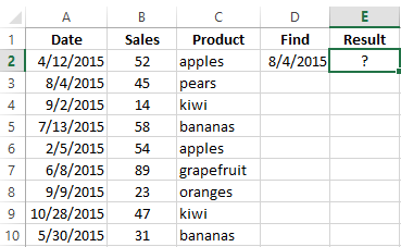
For the educational purposes, let’s take the table with the data:
| Formula | Description |
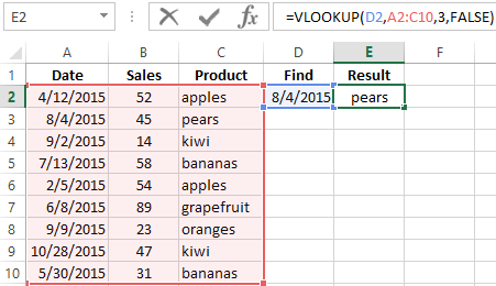
| =VLOOKUP(D2,A2:C10,3,FALSE) | The function searches for the value of the cell F5 in the range A2:C10 and returns the value of the cell F5, that was found in the column 3, the exact match. |
 |
|
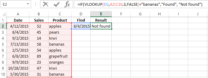
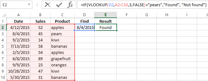
| =IF(VLOOKUP(D2,A$2:C$10,3,FALSE)=»bananas»,»Found», «Not found») | We need to find out whether bananas were sold 04. 08. 15. If bananas sold, the word «Found» appears in the corresponding cell. If bananas weren`t sold – «Not found». |
 |
|
| =IF(VLOOKUP(D2,A2:C10,3,FALSE)=»pears»,»Found», «Not found») | If the «bananas» are changed to «pears», the result will be «Found» |
 |
|
| =IFERROR(VLOOKUP(D2,A2:C10,3,FALSE),0) | When the VLOOKUP function can not find a value, it gives an error message # N/A. To avoid this, we use the function IFERROR. |
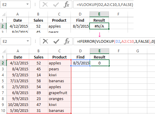 We will find out whether there were sales 08.05.15 |
|
| =VLOOKUP(A2,[employees.xlsx]Sheet1!A2:B10,2,FALSE) | If it`s necessary to implement for the search value in the another Excel workbook, then when filling out the «table» argument, we go to another workbook and select the desired range with the data. |
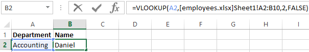 We wanted to know who worked 06. 08.15. |
|
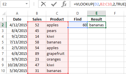
| =VLOOKUP(D2,B2:C10,2,TRUE) | The searching of the approximate value. |
 |
It is important:
- The VLOOKUP function always searches for data in the leftmost column of the table with values.
- The register is not taken into account: small and large letters for Excel are the same.
- If the sought after is less than the minimum value in the array, the program will return the error # N/D.
- If you set the column number to 0, the function will show #VALUE. If the third argument is greater than the number of columns in the table — #REFERENCE.
- To copy the correct array, we apply to the absolute references (F4 key).
How to use by the HLOOKUP function in Excel: examples
For educational purposes, let`s take the following table:
| Formula | Description |
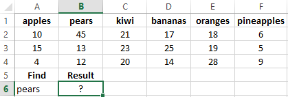
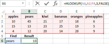
| =HLOOKUP(A6,A1:F4,3,FALSE) | Find the value of the cell |16 and return of the value from the third row of the same column. |
 |
The application of HLOOKUP in practice is limited, inasmuch as the horizontal representation of the information is used very rarely.
The symbols of substitution in VLOOKUP and HLOOKUP functions
It happens that the user does not remember the exact name. By specifying the desired value, he can apply the wildcard characters:
- «?» – replaces any character in text or digital information;
- «*» – for replacing any sequence of characters.
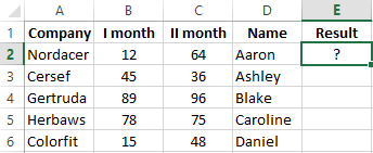
- Let`s find the text that begins or ends with a certain set of characters. For example we need to find the name of the company. We forgot it, but remember that it starts with Kol. The problem will be solved by the following formula:
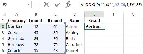
- We need to find the name of the company that ends with – «uda». The following formula will help:
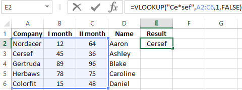
- Let`s find a company which name begins with «Ce» and ends with «sef». The formula of the VLOOKUP will look like this:
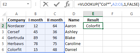
When the problems with memory are eliminated, you can work with data using all of the same functions.
How to compare sheets with the helping of VLOOKUP and HLOOKUP?
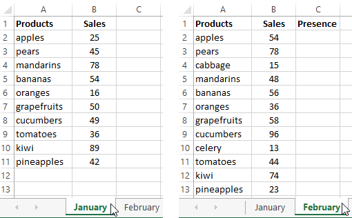
We have data about sales for January and February. These tables need to be compared using the formulas VLOOKUP and HLOOKUP. For clarity, we’ll put them in one sheet for now, but we will work in conditions when the ranges are in different sheets.
How can I compare sheets using VLOOKUP in Excel?
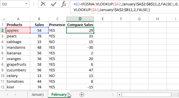
Let`s solve the problem 1: we compare the names of goods in January and February. Inasmuch as there are more of them in February, we will enter the formula on the «February» sheet.
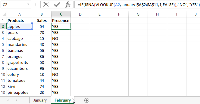
Let`s solve the problem 2: we compare the sales by positions in January and February. We use the following formula:
How can I compare sheets with HLOOKUP in Excel?
To demonstrate the action of the HLOOKUP function, we take two «horizontal» tables, located on different sheets.
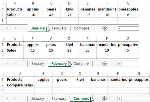
The task – is to compare sales by positions for January and February.
We create the new «Compare» sheet. This is not the obligatory condition. You can compare the data and display the difference on any sheet («January» or «February»).
The formula:
The result:
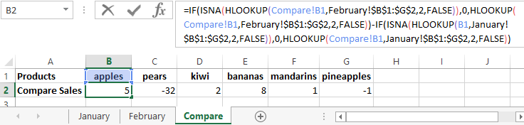
Let analyze the parts of the formula:
«Half» up to the sign «-»:
=IF(ISNA(HLOOKUP(Compare!B1,February!$B$1:$G$2,2,FALSE)),0,HLOOKUP(
Compare!B1,February!$B$1:$G$2,2,FALSE))-
The desired value – is the first cell in the table for comparison. The analyzed range – is the table with sales for February. The HLOOKUP function «takes» data from the second line in «accurate» reproduction.
After the «-» sign:
-IF(ISNA(HLOOKUP(B1,January!
$B$1:$G$2,2,FALSE)),0,HLOOKUP(Compare!B1,January!$B$1:$G$2,2,FALSE))
There are all the same in addition to the range. Here we take the table with sales for January.
Download example functions VLOOKUP and HLOOKUP
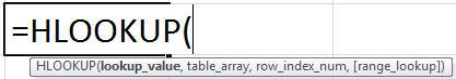
When we enter a formula, Excel prompts about: what the argument you need to enter now.
What is HLOOKUP in Excel?
The HLOOKUP function of Excel looks for the specified value in the topmost row of the table and returns another value from the same column of a different row. The specified value is called the lookup value and the value returned is known as a match. This match corresponds with either the exact lookup value (exact match) or with a value close to the lookup value (approximate match).
For example, cells A1 and B1 contain 10 and 20 respectively. Cells A2 and B2 contain “a” and “b” (without the double quotation marks) respectively. The formula “=HLOOKUP(10,A1:B2,2,0)” returns “a,” as shown in the following image.

The given HLOOKUP formula can be interpreted as follows:
- 10–HLOOKUP searches for this value.
- A1:B2–HLOOKUP searches in the topmost row of this array.
- 2–HLOOKUP returns a value from this row of the array.
- 0–HLOOKUP returns an exact match.
HLOOKUP stands for horizontal lookup in excel. It looks up values horizontally (in rows), unlike vertical lookup (VLOOKUPThe VLOOKUP excel function searches for a particular value and returns a corresponding match based on a unique identifier. A unique identifier is uniquely associated with all the records of the database. For instance, employee ID, student roll number, customer contact number, seller email address, etc., are unique identifiers.
read more), which looks up values vertically (in columns). Therefore, one must use the HLOOKUP when there is a need to search across (from left to right) in the topmost row of the array.
The purpose of using the HLOOKUP excel function is to quickly retrieve data based on certain predefined parameters. This function is categorized under the Lookup and Reference functions of Excel.
Table of contents
- What is HLOOKUP in Excel?
- Syntax of the HLOOKUP Function of Excel
- How to use the HLOOKUP Function in Excel?
- Example #1–Exact Match to Retrieve Numerical Values Including a Date
- Example #2–Exact and Approximate Match to Retrieve Percentages
- Errors Returned by the HLOOKUP Function in Excel
- The Key Points Related to the HLOOKUP Function in Excel
- Frequently Asked Questions
- HLOOKUP Function Video
- Recommended Articles
Syntax of the HLOOKUP Function of Excel
The syntax of the HLOOKUP function in excel is shown in the following image:
The HLOOKUP excel function accepts the following arguments:
- Lookup_value: This is the value to be searched. It can be a numeric value, text string or cell reference.
- Table_array: This consists of two or more rows where the lookup value is to be searched. It can be a range, table or named range. The lookup value must always be located in the topmost row of the “table_array.” Further, this topmost row can contain numeric values, text strings or logical values (true and false).
- Row_index_num: This is the exact row of the table array from which the match is to be returned. For instance, if the “row_index_num” is 3, a value from the third row of the table array is returned.
- Range_lookup: This can take either of the two logical values, which are described as follows:
- True (1): If the “range_lookup” is true or 1, the HLOOKUP returns an approximate match. Moreover, when this argument is set at true and an exact match is not found (refer to the succeeding note), the function returns the next largest value, which is less than the lookup value. If the “range_lookup” is true, the values of the table array must be sorted in an ascending order, beginning from left to right.
- False (0): If the “range_lookup” is false or 0, the HLOOKUP returns an exact match. Moreover, when this argument is set at false and an exact match is not found, the function returns the “#N/A” error. If the “range_lookup” is false, no sorting of the table array is required.
The arguments “lookup_value,” “table_array,” and “row_index_num” are mandatory, while the “range_lookup” is an optional argument. If the “range_lookup” argument is omitted, the HLOOKUP excel function assumes it as 1 (true).
Note: When the “range_lookup” argument is set at true, the HLOOKUP function searches for an exact match at first. If the exact match is not found, an approximate match is returned by the function. When the “range_lookup” argument is set at false, the HLOOKUP function searches for an exact match only.
How to use the HLOOKUP Function in Excel?
Let us consider some examples to understand the working of the HLOOKUPHLOOKUP function finds the data in the table’s first row and then provides a related value in the column aligned with the specified row. HLOOKUP examples enlighten the users on how to locate values when the data table is in horizontal form. read more function of Excel.
You can download this HLOOKUP Excel Template here – HLOOKUP Excel Template
Example #1–Exact Match to Retrieve Numerical Values Including a Date
The following image shows the sales revenue (row 6) generated and the profits (row 5) earned on particular dates (row 7) by an organization. This organization operates in four regions, namely, East, West, North, and South. The data for every region is shared. One column represents the data of one region.
We want to retrieve the profit, sales revenue, and the date of sales associated with the Northern region. Use the HLOOKUP function of Excel to perform a lookup with an exact match.
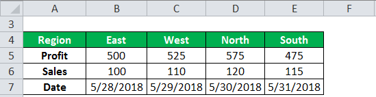
The steps to retrieve the data related to the Northern region are listed as follows:
Step 1: Enter the following formulas in cells B10, C10, and D10 respectively:
- “=HLOOKUP($A10,$A$4:$E$7,2,0)”
- “=HLOOKUP($A10,$A$4:$E$7,3,0)”
- “=HLOOKUP($A10,$A$4:$E$7,4,0)”
Cell A10 contains “north.”
Step 2: Press the “Enter” key after entering each formula in the preceding step. The outputs are shown in cells B10, C10, and D10 of the following image.

Explanation: In all the three formulas (entered in step 1), the HLOOKUP looks for the value in cell A10, which is “north.” This value is looked up in the topmost row of the array A4:E7. Since the “range_lookup” is 0 in all three formulas, the HLOOKUP excel function looks for an exact match.
In pointer “a” (of step 1), the HLOOKUP returns a value from row 2 of the table array. The column from which the match is returned is the same as that of the North region (column D). The value which corresponds with the stated row and column is 575. Hence, from the formula in pointer “a,” the output is 575. This is the profit of the Northern region.
Likewise, in pointers “b” and “c” (of step 1), the HLOOKUP returns a value from rows 3 and 4 of the table array (A4:E7) respectively. In both formulas, the value is returned from the column North (column D).
So, the corresponding matches for pointers “b” and “c” are 120 and 5/30/2018 respectively. The former match is the sales revenue generated, while the latter is the date of sales related to the Northern region.
Example #2–Exact and Approximate Match to Retrieve Percentages
The following image shows certain random dates (row 15) and percentages (row 16). We want to retrieve the following values:
- The percentage of 1-Jan by performing a lookup with an exact match
- The percentage of 2-Apr by performing a lookup with an approximate match
Use the HLOOKUP function of Excel. Note that all dates pertain to the year 2011.
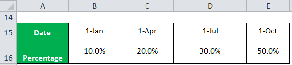
The steps to retrieve the given values are listed as follows:
Step 1: Enter the following formulas in cells B20 and B21 respectively:
- “=HLOOKUP(A20,A15:E16,2,0)” or “=HLOOKUP(A20,A15:E16,2,False)”
- “=HLOOKUP(A21,A15:E16,2,1)” or “=HLOOKUP(A20,A15:E16,2,True)”
Cells A20 and A21 contain “1-Jan” and “2-Apr” respectively.
Step 2: Press the “Enter” key after entering the preceding formulas. The outputs in cells B20 and B21 are 10.0% and 20.0% respectively. These are shown in the following image.
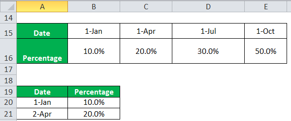
Explanation: In the formula of pointer “a” (entered in step 1), the HLOOKUP excel function looks for the value of cell A20 in the topmost row of the given table array (A15:E16). It looks for an exact match of the lookup value (1-Jan). This exact match is returned from the second row of the table array.
The column from which the exact match is returned is the same as that of 1-Jan (column B). Therefore, the corresponding value at the given row and column is 10.0%, which is the output of the first formula.
Likewise, in pointer “b” (of step 1), the HLOOKUP function searches for the value of cell A21, which is 2-Apr. This is also searched in the topmost row of the array A15:E16. However, this time the function looks for an approximate match as the “range_lookup” argument is set at 1 (or true).
The HLOOKUP excel function is unable to find an exact match of the lookup value (2-Apr) in the topmost row of the table array. So, the function returns the percentage corresponding to the next largest date, which is 1-Apr. This next largest date (1-Apr) is smaller than the lookup value (2-Apr).
Since the match needs to be from the second row of the given array (A15:E16), the output is 20.0%.
Note: The dates in cells B20 and B21 pertain to the same year (2011) as those given in the dataset. Had we entered the dates with different years, we would not have been able to retrieve the required data.
Errors Returned by the HLOOKUP Function in Excel
The errors returned by the HLOOKUP excel function are explained as follows:
a. “#N/A” error: This is returned if the “range_lookup” argument is set at false (or 0) and the HLOOKUP is unable to find the lookup value in the topmost row of the table array.
For instance, in the following image, the “lookup_value” is 2-Jan and an exact match is required. In cell B20, the formula “=HLOOKUP(A20,A15:E16,2,0)” returns the “#N/A” error.

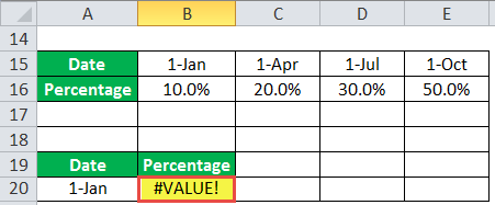
b. “#VALUE!” error: #VALUE! error#VALUE! Error in Excel represents that the reference cell the user has either entered an incorrect formula or used a wrong data type (mostly numerical data). Sometimes, it is difficult to identify the kind of mistake behind this error.read more is returned if the “row_index_num” entered is less than 1.
For instance, in the following image, the “row_index_num” is supplied as zero. In cell B20, the formula “=HLOOKUP(A20,A15:E16,0,0)” returns the “#VALUE!” error.
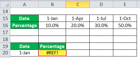
c. “#REF!” error: This is returned if the “row_index_num” entered is greater than the total rows of the table array.
For instance, in the following image, the “row_index_num” is supplied as 3, while the total rows of the “table_array” are 2. In cell B20, the formula “=HLOOKUP(A20,A15:E16,3,0)” returns the “#REF!” error.
The key points related to the HLOOKUP excel function are listed as follows:
- It is a case-insensitive function. This implies that the uppercase and lowercase values are treated the same.
- It is unable to look up anywhere else other than the topmost row of the table array. So, the lookup value should always be located in this row.
- It supports the usage of the wildcard characters like the asterisk (*) and question mark (?) in the “lookup_value” argument. In such cases, one can enter an incomplete text string as the “lookup_value” and, based on this, retrieve the corresponding value.
- It returns the first match in case there is more than one instance of the lookup value in the topmost row of the table array. To avoid such a situation, remove the duplicates before applying the HLOOKUP formula.
Note: If the lookup value is not located in the topmost row of the table array, a combination of the INDEX and MATCH functionsThe INDEX function can return the result from the row number, and the MATCH function can give us the position of the lookup value in the array. This combination of the INDEX MATCH is beneficial in addressing a fundamental limitation of VLOOKUP.read more can be used to fetch data.
Frequently Asked Questions
1. Define the HLOOKUP function and state when it should be used in Excel.
The HLOOKUP function of Excel searches a specified lookup value in the first row of an array and returns a corresponding match from another row. The column from which the match is returned is the same as that of the lookup value. In the arguments of the function, one can state whether an exact or an approximate match is required.
The HLOOKUP function is used in the following situations:
a. When the lookup value is located in the first row of the array
b. When the array is arranged horizontally and the value needs to be searched across a row of the worksheet
Note: For the syntax and the arguments of the HLOOKUP function, refer to the heading “Syntax of the HLOOKUP Function of Excel” of this article.
2. Describe the step-by-step usage of the HLOOKUP function in Excel.
The steps, when a single value needs to be fetched, are listed as follows:
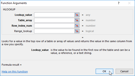
a. Type the arguments of the function manually in the cell where the output is required. Alternatively, from the Formulas tab, access the “insert function” dialog box. Select “HLOOKUP” from the “lookup & reference” functions. Enter the function arguments.
b. Press the “Enter” key if the arguments are entered manually in the preceding step. Alternatively, click “Ok” in the “function arguments” dialog box to proceed.
A single value is retrieved from the dataset.
The steps, when an array of values needs to be fetched, are listed as follows:
a. Select as many blank, horizontal cells as the number of rows required in the output.
b. In the first cell of the selection, enter the arguments of the HLOOKUP function manually. Ensure that the different row numbers of the “row_index_num” argument are entered within curly brackets {}. For instance, the formula should look like “=HLOOKUP(A1,A1:C3,{1,2,3},0).” Exclude the beginning and ending double quotation marks.
c. Press the keys “Ctrl+Shift+Enter” together.
An array of values is obtained in the blank row selected in step “a.”
3. How to perform HLOOKUP using a different Excel worksheet?
To extract data from a different worksheet, specify the sheet name followed by an exclamation mark. For instance, the HLOOKUP formula is stated as follows (ignore the beginning and ending double quotation marks):
“=HLOOKUP(A1,Sheet3!A1:C3,2,0)”
Here, the “lookup_value” is in cell A1. The “sheet3” contains the “table_array” A1:C3. The “row_index_num” is 2 and the “range_lookup” argument is 0.
If the name of the worksheet consists of non-alphabetical characters (like @, #, etc.) or spaces, enclose the name within single quotation marks followed by an exclamation mark (like ‘Sheet 3’! or ‘Sheet [email protected]’!).
Note: Rather than typing the arguments manually, one can select the cells of the different worksheet. Excel automatically inserts the sheet name in the HLOOKUP formula.
Likewise, to extract data from a different workbook, ensure that the name of the workbook is enclosed within square brackets. To make it easy, select the cells of the different workbook. Excel automatically inserts the names of the workbook and the worksheet in the HLOOKUP formula.
HLOOKUP Function Video
Recommended Articles
This has been a guide to the HLOOKUP in Excel. Here we discuss its formula and how to use the HLOOKUP function along with practical examples and downloadable Excel templates. You may also look at these useful functions of Excel –
- VLOOKUP with Two CriteriaVlookup and Hlookup are referencing functions in excel, used to reference data to match with a table array or a group of data and display the output. The difference between these referencing functions is that Vlookup uses reference columns while Hlookup uses reference rows.read more
- VLOOKUP Errors in Excel
- Power BI VlookupVLOOKUP in Power BI helps the users fetch data from the other tables. Since it is not an inbuilt function, the user needs to replicate it using the DAX function like the LOOKUPVALUE DAX function.read more
- Price Function in ExcelThe price function in Excel is a financial function that calculates the original value or face value of a stock for per 100 dollars, assuming interest is paid periodically.read more
![]()
Rohit Sharma is the Program Director for the UpGrad-IIIT Bangalore, PG Diploma Data Analytics Program.
Last Updated: Aug 24, 2022
·
6 min read
Home > Data Science > What is HLOOKUP in Excel? Function, Syntax & Examples
HLOOKUP in Excel is short for ‘Horizontal Lookup’. This function helps in searching for a certain value at the top of a row of a table, also known as a ‘table array’, to return a value from another specified row from the same column.
When comparison values are located in a row at the top of a table of data, and you need to look down a particular number of rows use the HLOOKUP function in Excel. VLOOKUP is a similar function when comparison values are located in a column located to the left of the specified data. Excel experts opine that the HLOOKUP formula is convenient and easy to use.
HLOOKUP is especially useful when working with data such as long lists. When working with columns containing multiple values in Excel, HLOOKUP makes it easy to associate target cells. HLOOKUP also enables us to automate changes in other associated cells by using the HLOOKUP function when you modify the target cell. HLOOKUP can also find partial matches, thus, proving to be extremely useful when we are not certain about our lookup values.
Here we will shed light on HLOOKUP in Excel and the HLOOKUP formula.
Learn online data science certifications from the World’s top Universities. Earn Executive PG Programs, Advanced Certificate Programs, or Masters Programs to fast-track your career.
How HLOOKUP Works
The HLOOKUP function is primarily used to retrieve a value from data located in a horizontal table. As mentioned before, it is similar to the “V” in the VLOOKUP function which is short for “vertical”.
To successfully use the HLOOKUP function, make sure that the lookup values are located in the first row of the table and are moving to the right horizontally. This function supports approximate and accurate matching and uses wildcards (* ?) to find partial matches.
Explore our Popular Data Science Courses
Syntax
The HLOOKUP function locates a value from the first row of a table. After locating a match, the value is retrieved from that column presenting the row given. The syntax for the HLOOKUP function is:-
The syntax of the HLOOKUP function in Excel has four elements. They are as follows:-
- Lookup_value: This is a mandated requirement in the HLOOKUP syntax. It locates the value you need to find in the first row of the table. Lookup_value can be a value, a text string, or a reference.
- Table_array: A table array is also a required element in the syntax of HLOOKUP. A table of information in which data is looked up. Always use a reference to a range name or a range.
- The values present in the first row of table_array can be numerical, alphabetical, or logical values.
- When the range_lookup is TRUE, the values located in the first row of table_array need to be placed in ascending order: -3, -2, -1, 0, 1, 2, A-Z; otherwise, HLOOKUP may not present the correct value. If range_lookup is FALSE, there is no need to sort the table_array.
- The lowercase and uppercase text are equal.
- Row_index_num: This is a crucial requirement as well. The matching value will be returned from this particular row number in table_array. A row_index_num of 1 returns a value in the first row of the table_array, and likewise, a row_index_num of 2 returns the value in the second row of the table_array, etc. If the row_index_num is more than the number of rows on table_array, HLOOKUP will return the #REF! error value and if the If row_index_num is lesser than 1, HLOOKUP will return the #VALUE! error value.
- Range_lookup: This is an optional element in the HLOOKUP syntax. It is a logical value that identifies if you want to find an accurate or an estimated match with HLOOKUP. If TRUE or omitted, you will get an estimated match, i.e., if HLOOKUP fails to find an accurate match, you will get the next largest value lesser than lookup_value. If FALSE, HLOOKUP will locate an exact match. If it fails to find a value, #N/A is the returned error value.
Example Of HLOOKUP in Excel
An HLOOKUP example for easy understanding:
To get a better experience of using the following example, it is advised to copy the example data in the following table and paste it into cell A1 in a fresh Excel worksheet. To see the results of the formulas, select them, press F2, and then click Enter.
| Apples | Oranges | Pears |
| 5 | 5 | 10 |
| 6 | 8 | 11 |
| 7 | 9 | 12 |
| Formula | Description | Result |
| =HLOOKUP(“Apples”, A1:C4, 2, TRUE) | Locates up “Apples” in row 1 and gives you the value from row 2 that’s in the same column (column A). | 5 |
| =HLOOKUP(“Oranges”, A1:C4, 3, FALSE) | Locates “Oranges” in row 1, and gives you the value from row 3 that’s in the same column (column B). | 8 |
| =HLOOKUP(“B”, A1:C4, 3, TRUE) | Locates “B” in row 1, and gives you the value from row 3 in the same column. This is because an accurate match for “B” is not found, and the largest value in row 1 less than “B” is used: “Apples,” in column A. | 6 |
| =HLOOKUP(“Pears”, A1:C4, 4) | Locates “Pears” in row 1, and gives you the value from row 4 in the same column (column C). | 12 |
| =HLOOKUP(3, {1,2,3;”a”,”b”,”c”;”d”,”e”,”f”}, 2, TRUE) | Locates the number 3 in the three-row array constant, and gives you the value from row 2 in the same column, which is in this case, third. You will find three rows of values in the array constant, where a semicolon separates each row (;). “c” is found in the second row and in the exact column as 3. Therefore “c” is returned. |
Important Things To Note About HLOOKUP
- HLOOKUP is a case-insensitive lookup. For example, it will consider “HAM” and “ham” the same.
- The ‘Lookup_value’ should be the first row of the ‘table_array’ while using HLOOKUP. To look somewhere else, another Excel formula needs to be used.
- Wildcard characters like ‘*’ or ‘?’ are supported by HLOOKUP in the ‘lookup_value’ argument if the ‘lookup_value’ is alphabetical.
- If HLOOKUP fails to locate the lookup_value, and the range_lookup is TRUE, the largest value lesser than the lookup_value is used.
- If lookup_value is < than the smallest value of table_array’s first row, HLOOKUP will generate the #N/A error value.
- If range_lookup is FALSE, the wildcard characters can be used as well.
Read our popular Data Science Articles
Conclusion
You can find the HLOOKUP function in every version of Microsoft Excel 2016, 2013, 2010, 2007, and lower. Having Microsoft Excel skills and proficiency in lookup functions can significantly boost your career.
Making a career in data analytics is a lucrative opportunity in the current industry. Data analysts work with huge volumes of data for extracting crucial information. To hone your skills in data analytics, you must join upGrad’s Data Analytics Certificate Program. Powered by Fullstack Academy, you will get a Caltech data analytics certificate upon completing the course. You will be able to learn data visualization skills, Python, and SQL through the course, which will pave your way for making a great data analyst.
What is the difference between HLOOKUP AND VLOOKUP?
The difference between HLOOKUP and VLOOKUP is that HLOOKUP searches for the target values inside the selected columns, whereas VLOOKUP searches for the target values inside the selected rows.
What is an alternative to HLOOKUP?
There are a few alternatives for HLOOKUP. XLOOKUP is a good alternative to HLOOKUP that allows you to search for values in both columns and rows.
Can you use HLOOKUP AND VLOOKUP together?
Yes, you can use both HLOOKUP and VLOOKUP together. You can use the two functions together through the nested function method. We can use a nested formula to combine the two functions and retrieve relevant values from structures such as tables.
Want to share this article?
