
Overview of formulas in Excel
Get started on how to create formulas and use built-in functions to perform calculations and solve problems.

Important: The calculated results of formulas and some Excel worksheet functions may differ slightly between a Windows PC using x86 or x86-64 architecture and a Windows RT PC using ARM architecture. Learn more about the differences.
Important: In this article we discuss XLOOKUP and VLOOKUP, which are similar. Try using the new XLOOKUP function, an improved version of VLOOKUP that works in any direction and returns exact matches by default, making it easier and more convenient to use than its predecessor.
Create a formula that refers to values in other cells
-
Select a cell.
-
Type the equal sign =.
Note: Formulas in Excel always begin with the equal sign.
-
Select a cell or type its address in the selected cell.

-
Enter an operator. For example, – for subtraction.
-
Select the next cell, or type its address in the selected cell.
-
Press Enter. The result of the calculation appears in the cell with the formula.


See a formula
-
When a formula is entered into a cell, it also appears in the Formula bar.
-
To see a formula, select a cell, and it will appear in the formula bar.


Enter a formula that contains a built-in function
-
Select an empty cell.
-
Type an equal sign = and then type a function. For example, =SUM for getting the total sales.
-
Type an opening parenthesis (.
-
Select the range of cells, and then type a closing parenthesis).
-
Press Enter to get the result.

Download our Formulas tutorial workbook
We’ve put together a Get started with Formulas workbook that you can download. If you’re new to Excel, or even if you have some experience with it, you can walk through Excel’s most common formulas in this tour. With real-world examples and helpful visuals, you’ll be able to Sum, Count, Average, and Vlookup like a pro.
Formulas in-depth
You can browse through the individual sections below to learn more about specific formula elements.
A formula can also contain any or all of the following: functions, references, operators, and constants.
Parts of a formula

1. Functions: The PI() function returns the value of pi: 3.142…
2. References: A2 returns the value in cell A2.
3. Constants: Numbers or text values entered directly into a formula, such as 2.
4. Operators: The ^ (caret) operator raises a number to a power, and the * (asterisk) operator multiplies numbers.
A constant is a value that is not calculated; it always stays the same. For example, the date 10/9/2008, the number 210, and the text «Quarterly Earnings» are all constants. An expression or a value resulting from an expression is not a constant. If you use constants in a formula instead of references to cells (for example, =30+70+110), the result changes only if you modify the formula. In general, it’s best to place constants in individual cells where they can be easily changed if needed, then reference those cells in formulas.
A reference identifies a cell or a range of cells on a worksheet, and tells Excel where to look for the values or data you want to use in a formula. You can use references to use data contained in different parts of a worksheet in one formula or use the value from one cell in several formulas. You can also refer to cells on other sheets in the same workbook, and to other workbooks. References to cells in other workbooks are called links or external references.
-
The A1 reference style
By default, Excel uses the A1 reference style, which refers to columns with letters (A through XFD, for a total of 16,384 columns) and refers to rows with numbers (1 through 1,048,576). These letters and numbers are called row and column headings. To refer to a cell, enter the column letter followed by the row number. For example, B2 refers to the cell at the intersection of column B and row 2.
To refer to
Use
The cell in column A and row 10
A10
The range of cells in column A and rows 10 through 20
A10:A20
The range of cells in row 15 and columns B through E
B15:E15
All cells in row 5
5:5
All cells in rows 5 through 10
5:10
All cells in column H
H:H
All cells in columns H through J
H:J
The range of cells in columns A through E and rows 10 through 20
A10:E20
-
Making a reference to a cell or a range of cells on another worksheet in the same workbook
In the following example, the AVERAGE function calculates the average value for the range B1:B10 on the worksheet named Marketing in the same workbook.
1. Refers to the worksheet named Marketing
2. Refers to the range of cells from B1 to B10
3. The exclamation point (!) Separates the worksheet reference from the cell range reference
Note: If the referenced worksheet has spaces or numbers in it, then you need to add apostrophes (‘) before and after the worksheet name, like =’123′!A1 or =’January Revenue’!A1.
-
The difference between absolute, relative and mixed references
-
Relative references A relative cell reference in a formula, such as A1, is based on the relative position of the cell that contains the formula and the cell the reference refers to. If the position of the cell that contains the formula changes, the reference is changed. If you copy or fill the formula across rows or down columns, the reference automatically adjusts. By default, new formulas use relative references. For example, if you copy or fill a relative reference in cell B2 to cell B3, it automatically adjusts from =A1 to =A2.
Copied formula with relative reference
-
Absolute references An absolute cell reference in a formula, such as $A$1, always refer to a cell in a specific location. If the position of the cell that contains the formula changes, the absolute reference remains the same. If you copy or fill the formula across rows or down columns, the absolute reference does not adjust. By default, new formulas use relative references, so you may need to switch them to absolute references. For example, if you copy or fill an absolute reference in cell B2 to cell B3, it stays the same in both cells: =$A$1.
Copied formula with absolute reference
-
Mixed references A mixed reference has either an absolute column and relative row, or absolute row and relative column. An absolute column reference takes the form $A1, $B1, and so on. An absolute row reference takes the form A$1, B$1, and so on. If the position of the cell that contains the formula changes, the relative reference is changed, and the absolute reference does not change. If you copy or fill the formula across rows or down columns, the relative reference automatically adjusts, and the absolute reference does not adjust. For example, if you copy or fill a mixed reference from cell A2 to B3, it adjusts from =A$1 to =B$1.
Copied formula with mixed reference
-
-
The 3-D reference style
Conveniently referencing multiple worksheets If you want to analyze data in the same cell or range of cells on multiple worksheets within a workbook, use a 3-D reference. A 3-D reference includes the cell or range reference, preceded by a range of worksheet names. Excel uses any worksheets stored between the starting and ending names of the reference. For example, =SUM(Sheet2:Sheet13!B5) adds all the values contained in cell B5 on all the worksheets between and including Sheet 2 and Sheet 13.
-
You can use 3-D references to refer to cells on other sheets, to define names, and to create formulas by using the following functions: SUM, AVERAGE, AVERAGEA, COUNT, COUNTA, MAX, MAXA, MIN, MINA, PRODUCT, STDEV.P, STDEV.S, STDEVA, STDEVPA, VAR.P, VAR.S, VARA, and VARPA.
-
3-D references cannot be used in array formulas.
-
3-D references cannot be used with the intersection operator (a single space) or in formulas that use implicit intersection.
What occurs when you move, copy, insert, or delete worksheets The following examples explain what happens when you move, copy, insert, or delete worksheets that are included in a 3-D reference. The examples use the formula =SUM(Sheet2:Sheet6!A2:A5) to add cells A2 through A5 on worksheets 2 through 6.
-
Insert or copy If you insert or copy sheets between Sheet2 and Sheet6 (the endpoints in this example), Excel includes all values in cells A2 through A5 from the added sheets in the calculations.
-
Delete If you delete sheets between Sheet2 and Sheet6, Excel removes their values from the calculation.
-
Move If you move sheets from between Sheet2 and Sheet6 to a location outside the referenced sheet range, Excel removes their values from the calculation.
-
Move an endpoint If you move Sheet2 or Sheet6 to another location in the same workbook, Excel adjusts the calculation to accommodate the new range of sheets between them.
-
Delete an endpoint If you delete Sheet2 or Sheet6, Excel adjusts the calculation to accommodate the range of sheets between them.
-
-
The R1C1 reference style
You can also use a reference style where both the rows and the columns on the worksheet are numbered. The R1C1 reference style is useful for computing row and column positions in macros. In the R1C1 style, Excel indicates the location of a cell with an «R» followed by a row number and a «C» followed by a column number.
Reference
Meaning
R[-2]C
A relative reference to the cell two rows up and in the same column
R[2]C[2]
A relative reference to the cell two rows down and two columns to the right
R2C2
An absolute reference to the cell in the second row and in the second column
R[-1]
A relative reference to the entire row above the active cell
R
An absolute reference to the current row
When you record a macro, Excel records some commands by using the R1C1 reference style. For example, if you record a command, such as clicking the AutoSum button to insert a formula that adds a range of cells, Excel records the formula by using R1C1 style, not A1 style, references.
You can turn the R1C1 reference style on or off by setting or clearing the R1C1 reference style check box under the Working with formulas section in the Formulas category of the Options dialog box. To display this dialog box, click the File tab.
Top of Page


Need more help?
You can always ask an expert in the Excel Tech Community or get support in the Answers community.
See Also
Switch between relative, absolute and mixed references for functions
Using calculation operators in Excel formulas
The order in which Excel performs operations in formulas
Using functions and nested functions in Excel formulas
Define and use names in formulas
Guidelines and examples of array formulas
Delete or remove a formula
How to avoid broken formulas
Find and correct errors in formulas
Excel keyboard shortcuts and function keys
Excel functions (by category)
Need more help?
Want more options?
Explore subscription benefits, browse training courses, learn how to secure your device, and more.
Communities help you ask and answer questions, give feedback, and hear from experts with rich knowledge.
Formulas and functions are the building blocks of working with numeric data in Excel. This article introduces you to formulas and functions.
In this article, we will cover the following topics.
- What is Formulas in Excel?
- Mistakes to avoid when working with formulas in Excel
- What is Function in Excel?
- The importance of functions
- Common functions
- Numeric Functions
- String functions
- Date Time functions
- V Lookup function
Tutorials Data
For this tutorial, we will work with the following datasets.
Home supplies budget
| S/N | ITEM | QTY | PRICE | SUBTOTAL | Is it Affordable? |
|---|---|---|---|---|---|
| 1 | Mangoes | 9 | 600 | ||
| 2 | Oranges | 3 | 1200 | ||
| 3 | Tomatoes | 1 | 2500 | ||
| 4 | Cooking Oil | 5 | 6500 | ||
| 5 | Tonic Water | 13 | 3900 |
House Building Project Schedule
| S/N | ITEM | START DATE | END DATE | DURATION (DAYS) |
|---|---|---|---|---|
| 1 | Survey land | 04/02/2015 | 07/02/2015 | |
| 2 | Lay Foundation | 10/02/2015 | 15/02/2015 | |
| 3 | Roofing | 27/02/2015 | 03/03/2015 | |
| 4 | Painting | 09/03/2015 | 21/03/2015 |
What is Formulas in Excel?
FORMULAS IN EXCEL is an expression that operates on values in a range of cell addresses and operators. For example, =A1+A2+A3, which finds the sum of the range of values from cell A1 to cell A3. An example of a formula made up of discrete values like =6*3.
=A2 * D2 / 2
HERE,
"="tells Excel that this is a formula, and it should evaluate it."A2" * D2"makes reference to cell addresses A2 and D2 then multiplies the values found in these cell addresses."/"is the division arithmetic operator"2"is a discrete value
Formulas practical exercise
We will work with the sample data for the home budget to calculate the subtotal.
- Create a new workbook in Excel
- Enter the data shown in the home supplies budget above.
- Your worksheet should look as follows.

We will now write the formula that calculates the subtotal
Set the focus to cell E4
Enter the following formula.
=C4*D4
HERE,
"C4*D4"uses the arithmetic operator multiplication (*) to multiply the value of the cell address C4 and D4.
Press enter key
You will get the following result

The following animated image shows you how to auto select cell address and apply the same formula to other rows.

Mistakes to avoid when working with formulas in Excel
- Remember the rules of Brackets of Division, Multiplication, Addition, & Subtraction (BODMAS). This means expressions are brackets are evaluated first. For arithmetic operators, the division is evaluated first followed by multiplication then addition and subtraction is the last one to be evaluated. Using this rule, we can rewrite the above formula as =(A2 * D2) / 2. This will ensure that A2 and D2 are first evaluated then divided by two.
- Excel spreadsheet formulas usually work with numeric data; you can take advantage of data validation to specify the type of data that should be accepted by a cell i.e. numbers only.
- To ensure that you are working with the correct cell addresses referenced in the formulas, you can press F2 on the keyboard. This will highlight the cell addresses used in the formula, and you can cross check to ensure they are the desired cell addresses.
- When you are working with many rows, you can use serial numbers for all the rows and have a record count at the bottom of the sheet. You should compare the serial number count with the record total to ensure that your formulas included all the rows.
Check Out
Top 10 Excel Spreadsheet Formulas
What is Function in Excel?
FUNCTION IN EXCEL is a predefined formula that is used for specific values in a particular order. Function is used for quick tasks like finding the sum, count, average, maximum value, and minimum values for a range of cells. For example, cell A3 below contains the SUM function which calculates the sum of the range A1:A2.
- SUM for summation of a range of numbers
- AVERAGE for calculating the average of a given range of numbers
- COUNT for counting the number of items in a given range
The importance of functions
Functions increase user productivity when working with excel. Let’s say you would like to get the grand total for the above home supplies budget. To make it simpler, you can use a formula to get the grand total. Using a formula, you would have to reference the cells E4 through to E8 one by one. You would have to use the following formula.
= E4 + E5 + E6 + E7 + E8
With a function, you would write the above formula as
=SUM (E4:E8)
As you can see from the above function used to get the sum of a range of cells, it is much more efficient to use a function to get the sum than using the formula which will have to reference a lot of cells.
Common functions
Let’s look at some of the most commonly used functions in ms excel formulas. We will start with statistical functions.
| S/N | FUNCTION | CATEGORY | DESCRIPTION | USAGE |
|---|---|---|---|---|
| 01 | SUM | Math & Trig | Adds all the values in a range of cells | =SUM(E4:E8) |
| 02 | MIN | Statistical | Finds the minimum value in a range of cells | =MIN(E4:E8) |
| 03 | MAX | Statistical | Finds the maximum value in a range of cells | =MAX(E4:E8) |
| 04 | AVERAGE | Statistical | Calculates the average value in a range of cells | =AVERAGE(E4:E8) |
| 05 | COUNT | Statistical | Counts the number of cells in a range of cells | =COUNT(E4:E8) |
| 06 | LEN | Text | Returns the number of characters in a string text | =LEN(B7) |
| 07 | SUMIF | Math & Trig |
Adds all the values in a range of cells that meet a specified criteria. =SUMIF(range,criteria,[sum_range]) |
=SUMIF(D4:D8,”>=1000″,C4:C8) |
| 08 | AVERAGEIF | Statistical |
Calculates the average value in a range of cells that meet the specified criteria. =AVERAGEIF(range,criteria,[average_range]) |
=AVERAGEIF(F4:F8,”Yes”,E4:E8) |
| 09 | DAYS | Date & Time | Returns the number of days between two dates | =DAYS(D4,C4) |
| 10 | NOW | Date & Time | Returns the current system date and time | =NOW() |
Numeric Functions
As the name suggests, these functions operate on numeric data. The following table shows some of the common numeric functions.
| S/N | FUNCTION | CATEGORY | DESCRIPTION | USAGE |
|---|---|---|---|---|
| 1 | ISNUMBER | Information | Returns True if the supplied value is numeric and False if it is not numeric | =ISNUMBER(A3) |
| 2 | RAND | Math & Trig | Generates a random number between 0 and 1 | =RAND() |
| 3 | ROUND | Math & Trig | Rounds off a decimal value to the specified number of decimal points | =ROUND(3.14455,2) |
| 4 | MEDIAN | Statistical | Returns the number in the middle of the set of given numbers | =MEDIAN(3,4,5,2,5) |
| 5 | PI | Math & Trig | Returns the value of Math Function PI(π) | =PI() |
| 6 | POWER | Math & Trig |
Returns the result of a number raised to a power. POWER( number, power ) |
=POWER(2,4) |
| 7 | MOD | Math & Trig | Returns the Remainder when you divide two numbers | =MOD(10,3) |
| 8 | ROMAN | Math & Trig | Converts a number to roman numerals | =ROMAN(1984) |
String functions
These basic excel functions are used to manipulate text data. The following table shows some of the common string functions.
| S/N | FUNCTION | CATEGORY | DESCRIPTION | USAGE | COMMENT |
|---|---|---|---|---|---|
| 1 | LEFT | Text | Returns a number of specified characters from the start (left-hand side) of a string | =LEFT(“GURU99”,4) | Left 4 Characters of “GURU99” |
| 2 | RIGHT | Text | Returns a number of specified characters from the end (right-hand side) of a string | =RIGHT(“GURU99”,2) | Right 2 Characters of “GURU99” |
| 3 | MID | Text |
Retrieves a number of characters from the middle of a string from a specified start position and length. =MID (text, start_num, num_chars) |
=MID(“GURU99”,2,3) | Retrieving Characters 2 to 5 |
| 4 | ISTEXT | Information | Returns True if the supplied parameter is Text | =ISTEXT(value) | value – The value to check. |
| 5 | FIND | Text |
Returns the starting position of a text string within another text string. This function is case-sensitive. =FIND(find_text, within_text, [start_num]) |
=FIND(“oo”,”Roofing”,1) | Find oo in “Roofing”, Result is 2 |
| 6 | REPLACE | Text |
Replaces part of a string with another specified string. =REPLACE (old_text, start_num, num_chars, new_text) |
=REPLACE(“Roofing”,2,2,”xx”) | Replace “oo” with “xx” |
Date Time Functions
These functions are used to manipulate date values. The following table shows some of the common date functions
| S/N | FUNCTION | CATEGORY | DESCRIPTION | USAGE |
|---|---|---|---|---|
| 1 | DATE | Date & Time | Returns the number that represents the date in excel code | =DATE(2015,2,4) |
| 2 | DAYS | Date & Time | Find the number of days between two dates | =DAYS(D6,C6) |
| 3 | MONTH | Date & Time | Returns the month from a date value | =MONTH(“4/2/2015”) |
| 4 | MINUTE | Date & Time | Returns the minutes from a time value | =MINUTE(“12:31”) |
| 5 | YEAR | Date & Time | Returns the year from a date value | =YEAR(“04/02/2015”) |
VLOOKUP function
The VLOOKUP function is used to perform a vertical look up in the left most column and return a value in the same row from a column that you specify. Let’s explain this in a layman’s language. The home supplies budget has a serial number column that uniquely identifies each item in the budget. Suppose you have the item serial number, and you would like to know the item description, you can use the VLOOKUP function. Here is how the VLOOKUP function would work.

=VLOOKUP (C12, A4:B8, 2, FALSE)
HERE,
"=VLOOKUP"calls the vertical lookup function"C12"specifies the value to be looked up in the left most column"A4:B8"specifies the table array with the data"2"specifies the column number with the row value to be returned by the VLOOKUP function"FALSE,"tells the VLOOKUP function that we are looking for an exact match of the supplied look up value
The animated image below shows this in action

Download the above Excel Code
Summary
Excel allows you to manipulate the data using formulas and/or functions. Functions are generally more productive compared to writing formulas. Functions are also more accurate compared to formulas because the margin of making mistakes is very minimum.
Here is a list of important Excel Formula and Function
- SUM function =
=SUM(E4:E8)
- MIN function =
=MIN(E4:E8)
- MAX function =
=MAX(E4:E8)
- AVERAGE function =
=AVERAGE(E4:E8)
- COUNT function =
=COUNT(E4:E8)
- DAYS function =
=DAYS(D4,C4)
- VLOOKUP function =
=VLOOKUP (C12, A4:B8, 2, FALSE)
- DATE function =
=DATE(2020,2,4)
Home / What is a Function in Excel
Home / What is a Function in Excel
What is a Function in Excel
In Excel, a function is a predefined formula that performs a specific calculation by using values a user input as arguments. Every Excel function has a specific purpose, in simple words, it calculates a specific value. Each function has its arguments (the value one needs to input) to get the result value in the cell.
Components
Each function has two major components. In short, each function (except a few) is made up of two following things:
- Function Name
- Arguments
Let me show you an example. Let’s take a look at the below function which we have inserted in the cell A1.
Now if you look at the formula bar you can understand the structure of the function by splitting it into two parts i.e. name and arguments.
Function Arguments
As I have already mentioned that in a function you need to specify input values to get the desired result. An argument is that value which you need to specify. If you look at the syntax of a function you can see there in each function there is set arguments to specify.
Below are the types of arguments:
- Required: A required argument is compulsory for a user to specify and without which a function can’t calculate its result.
- Optional: If you skip specifying these arguments it will not stop a function to calculate its result value.
- No Arguments: There are few functions (like NOW) where you don’t need to specify any argument.
How to INSERT a Function in Excel
The easiest way to insert a function in a cell in Excel is to type the name of the function you want to insert starting with equals to sign.
Let’s say you want to insert the SUM function:
- First of all, you need to type = and the then type SUM.
- After that, enter the opening parentheses.
- Specify the arguments (refer to a cell or you can directly enter values into the function).
- In the end, type closing parentheses and hit enter.
Major Types
Below are the major types:
- Text Functions: If you deal with data where you have text, then below are some of the functions which you need to learn to work efficiently.
- Date Functions: Dates are one of the major ingredients of data that you use every day, and helps you to analyze your data in a better way.
- Time Functions: Just like dates, time is could also be there in data and you can use time functions to deal with data where you have time values.
- Logical Functions: Logical functions can help you create some of the most helpful formula in your spreadsheet.
- Maths Functions: Excel is all about calculations and analysis, and mathematical functions and you can use these functions to get better in calculations and analysis.
- Statistical Functions: One of the best things about Excel is there are a bunch of statistical functions there that you can use to analyze data easily.
- Lookup Functions: In Excel, there some specific functions which can help you to look up a value or specific information about a cell or a range of cells.
- Information Function: These some specific functions which you can use to get information about the values you supplied.
- Financial Functions: These functions can help you calculate some of the common but important financial calculations in an easy way.
About the Author

Puneet is using Excel since his college days. He helped thousands of people to understand the power of the spreadsheets and learn Microsoft Excel. You can find him online, tweeting about Excel, on a running track, or sometimes hiking up a mountain.
Data comes to use only when you can actually work on it and Excel is one tool that provides a great amount of convenience both when you have to formulate equations of your own or make use of the built-in ones. In this article, you will be learning how you can actually work with these Excel Formulas ad Functions.
Here is a quick look at the topics that are discussed over here:
- What is a Formula?
- Writing Excel Formulas
- Editing a Formula
- Copy/ Paste a Formula
- Hide Formulas in Excel
- Operator Precedence Excel Formulas
- What are Functions in Excel?
- Most Important Functions
What is a Formula?
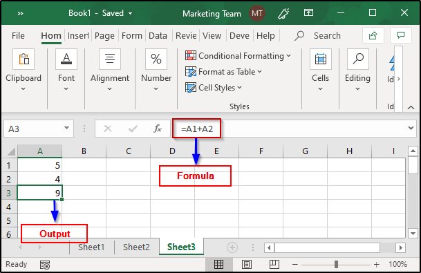
In general, a formula is a condensed way of representing some information in terms of symbols. In Excel, formulas are expressions that can be entered into the cells of an Excel sheet and their outputs are displayed as a result.
Excel formulas can be of the following types:
|
Type |
Example |
Description |
|
Mathematical operators( +, -, *, etc) |
Example: =A1+B1 |
Adds the values of A1 and B1 |
|
Values or text |
Example: 100*0.5 multiples 100 times 0.5 |
Takes the values and returns the output |
|
Cell reference |
EXAMPLE: =A1=B1 |
Returns TRUE or FALSE by comparing A1 and B1 |
|
Worksheet functions |
EXAMPLE: =SUM(A1: B1) |
Returns the output by adding values present in A1 and B1 |
Writing Excel Formulas:
In order to write a formula to an Excel sheet cell, you can do as follows:
- Select the cell where you want the result to be displayed
- Type a “=” sign initially to let Excel know that you are going to enter a formula in that cell
- After that, you can either type the cell addresses or specify the values that you intend to calculate
- For example, if you want to add the values of two cells, you can type in the cell address as follows:
- You can also select the cells whose sum you want to calculate by selecting all the required cells while pressing down the Ctrl key:

Editing a Formula:
In case you want to edit some previously entered formula, simply select the cell that contains the target formula and in the formula bar you can make the desired changes. In the previous example, I have calculated the Sum of A1 and A2. Now, I will edit the same and change the formula to calculate the product of the values present in these two cells:
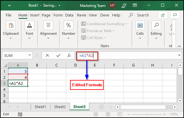
Once this is done, press Enter to see the desired output.
Copy or Paste a Formula:
Excel comes in really handy when you have to copy/ paste formulas. Whenever you copy a formula, Excel automatically takes care of the cell references that are required at that position. This is done through a system called as Relative Cell Addresses.
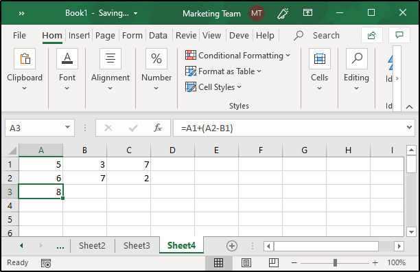
To copy a formula, select the cell that holds the original formula and then drag it till that cell which requires a copy of that formula as follows:
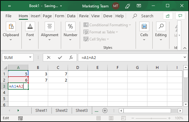
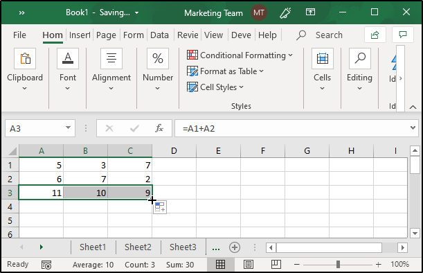
As you can see in the image, the formula is written originally in A3 and then I have dragged it down along B3 and C3 to calculate the sum of B1, B2 and C1, C2 without exclusively writing down the cell addresses.
In case I change the values of any of the cells, the output will be updated automatically by Excel in accordance with the Relative Cell Addresses, Absolute Cell Addresses or Mixed Cell Addresses.
Hide Formulas in Excel:
In case you want to hide some formula from an excel sheet, you can do it as follows:
- Select the cells whose formula you intend to hide
- Open the Font window and select the Protection pane
- Check the Hidden option and click on OK
- Then, from the ribbon tab, select Review
- Click on Protect sheet (Formulas will not work if you do not do this)
- Excel will ask you to enter a password in order to unhide the formulas for future use
Operator Precedence of Excel Formulas:
Excel formulas follow the BODMAS (Brackets Order Division Multiplication Addition Subtraction) rules. If you have a formula that contains brackets, the expression within the brackets will be solved before any other part of the complete formula. Take a look at the image below:
As you can see in the above example, I have a formula that consists of a bracket. So in accordance with the BODMAS rules, Excel will first find the difference between A2 and B1 and then it adds the result with A1.
What are ‘Functions’ in Excel?
In general, a function defines a formula that is executed in some given order. Excel provides a huge number of built-in functions that can be used in order to calculate the result of various formulas.
Formulas in Excel are divided into the following categories:
| Catagory | Important Formulas |
|
Date & Time |
DATE, DAY, MONTH, HOUR, etc |
|
Financial |
ACCINT, ACCINTM, DOLLARDE, INTRAATE, etc |
|
Math & Trig |
SUM, SUMIF, PRODUCT, SIN, COS, etc |
|
Statistical |
AVERAGE, COUNT, COUNTIF, MAX, MIN, etc |
|
Lookup & Reference |
COLUMN, HLOOKUP, ROW, VLOOKUP, CHOOSE, etc |
|
Database |
DAVERAGE, DCOUNT, DMIN, DMAX, etc |
|
Text |
BAHTTEXT, DOLLAR, LOWER, UPPER, etc |
|
Logical |
AND, OR, NOT, IF, TRUE, FALSE, etc |
|
Information |
INFO, ERROR.TYPE, TYPE, ISERROR, etc |
|
Engineering |
COMPLEX, CONVERT, DELTA, OCT2BIN, etc |
|
Cube |
CUBESET, CUBENUMBER, CUBEVALUE, etc |
|
Compatibility |
PERCENTILE, RANK, VAR, MODE, etc |
|
Web |
ENCODEURL, FILTERXML, WEBSERVICE |
Now, let us check out how to make use of some of the most important and commonly used Excel Formulas.
Most Important Excel Functions:
Here are some of the most important Excel functions along with their descriptions and examples.
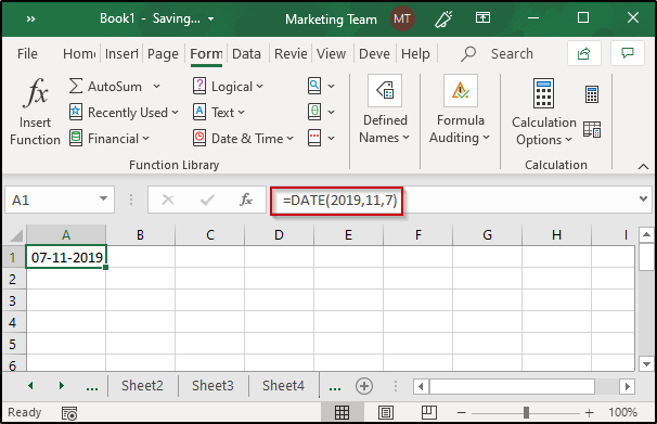
DATE:
One of the most important and widely used Date function in Excel is the DATE function. The syntax of it is as follows:
DATE(year, month, day)
This function returns a number that represents the given date in the MS Excel date-time format. The DATE function can be used as follows:
EXAMPLE:
- =DATE(2019,11,7)
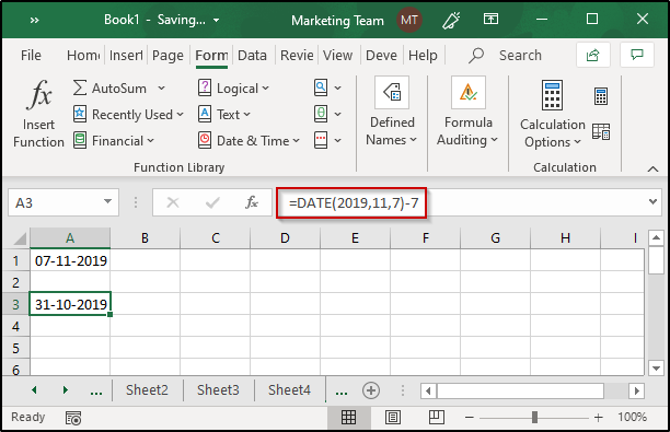
- =DATE(2019,11,7)-7 (returns the current date – seven days)
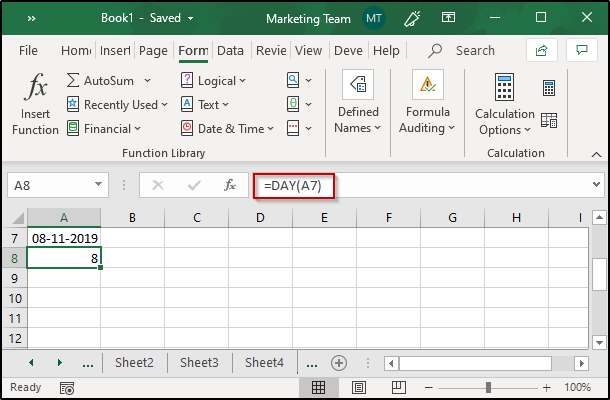
DAY:
This function returns the day value of the month (1-31). The syntax of it is as follows:
DAY(serial_number)
Here, serial_number is the date whose day you want to retrieve. It can be given in any manner such as the result of some other function, supplied by the DATE function, or a cell reference.
EXAMPLE:
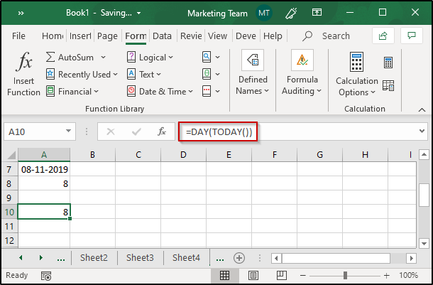
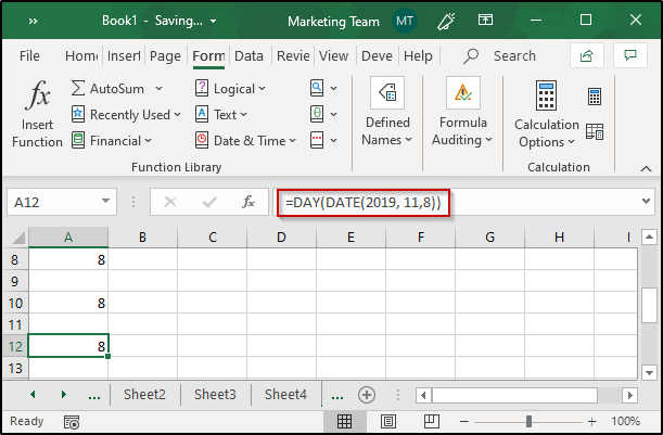
- =DAY(A7)
- =DAY(TODAY())
- =DAY(DATE(2019, 11,8))
MONTH:
Just like the DAY function, Excel provides another function i.e the MONTH function to retrieve the month from a specific date. The syntax is as follows:
MONTH(serial_number)
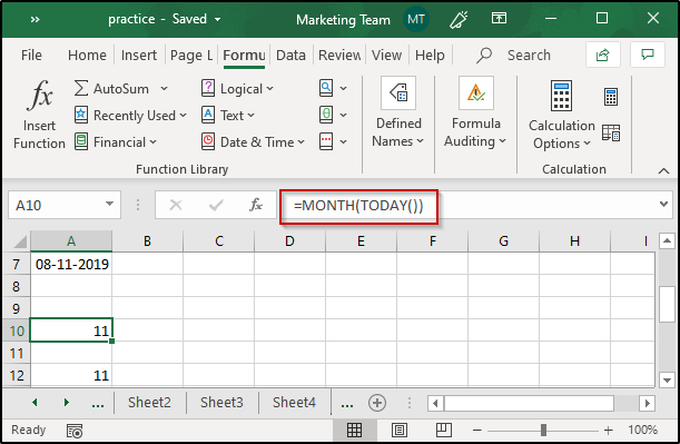
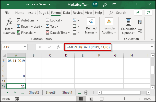
EXAMPLE:
- =MONTH(TODAY())
- =MONTH(DATE(2019, 11,8))
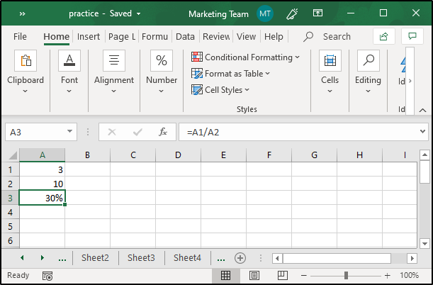
Percentage:
As we all know, Percentage is the ratio calculated as a fraction of 100. It can be denoted as follows:
Percentage = (Part/ Whole) x 100
In Excel, you can calculate the percentage of any desired values. For example, if you have the part and whole values present in A1 and A2 and you want to calculate the percentage, you can do it as follows:
- Select the cell where you want to display the result
- Type “=” sign
- Then, type in the formula as A1/ A2 and hit Enter
- From the home tab numbers group, select the “%” symbol
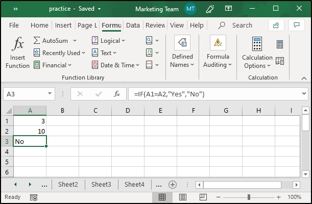
IF:
The IF statement is a conditional statement that returns True when the specified condition is satisfied and Flase when the condition is not. Excel provides a built-in “IF” function that serves this purpose. Its syntax is as follows:
IF(logical_test, value_if_true, value_if_false)
Here, logical_test is the condition that is to be checked
EXAMPLE:
- Enter the values to be compared
- Select the cell that will display the output
- Type in the Formula Bar “=IF(A1=A2, “Yes”, “No”)” and hit enter
VLOOKUP:
This function is used in order to look up and fetch some particular data from a column from an Excel sheet. The “V” in VLOOKUP stands for vertical lookup. It is one of the most important and widely used formulas in Excel and in order to use this function, the table must be sorted in ascending order. The syntax of this function is as follows:
VLOOKUP(lookup_value, table_array, col_index, num_range, lookup)
where,
lookup_value is the value to be searched
table_array is the table that is to be searched
col_index is the column from which the value is to be retrieved
range_lookup (optional) returns TRUE for approx. match and FALSE for an exact match
EXAMPLE:
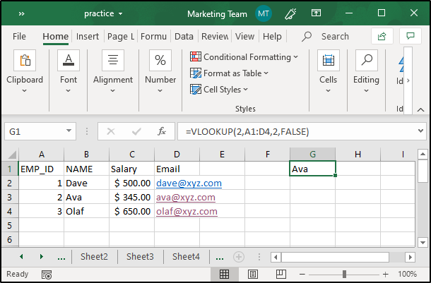
As you can see in the image, the value that I have specified is 2 and the table range is between A1 and D4. I want to fetch the name of the employee, therefore I have given the column value as 2 and since I want it to be an exact match, I used False for range lookup.
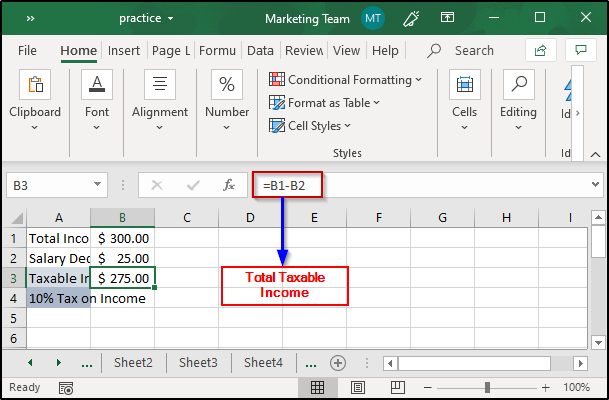
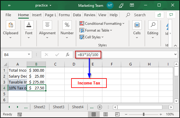
Income Tax:
Suppose you want to calculate the income tax of a person whose total salary is $300. You will need to calculate the income tax as follows:
- List down the Total Salary, Salary Deductions, Taxable Income and the percentage of Tax on Income
- Specify the values of Total Salary, Salary Deductions
- Then calculate the Taxable Income by finding the difference between Total Salary and Salary Deductions
- Finally, calculate the Tax Amount
SUM:
The SUM function in Excel calculates the result by adding all the specified values in Excel. The syntax of this function is as follows:
SUM(number1, number2, …)
Adds all the numbers that are specified as a parameter to it.
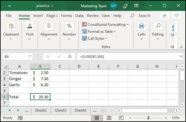
EXAMPLE:
In case you want to calculate the sum of the amount you spent in purchasing vegetables, list down all the prices and then use the SUM formula as follows:
Compound Interest:
To calculate compound interest, you can make use of one of the Excel Formulas called FV. This function will return the future value of an investment on the basis of periodic, constant interest rate and payments. The syntax of this function is as follows:
FV(rate, nper, pmt, pv, type)
In order to calculate the rate, you will need to divide the annual rate by the number of periods i.e annual rate/ periods. No. of periods or nper is calculated by multiplying the term (no. of years) with the periods i.e term * periods. pmt stands for periodic payment and can be any value including zero.
Consider the following example:
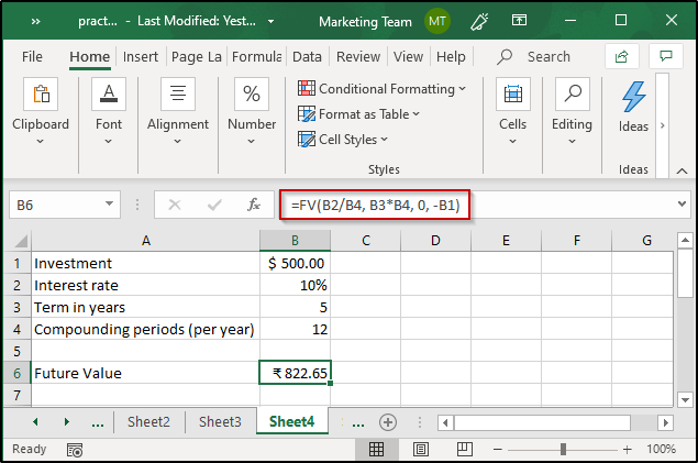
In the above example, I have calculated the Compound Interest for $500 at a rate of 10% for 5 years and assuming that the periodic payment value is 0. Please note that I have used -B1 meaning, $500 has been taken from me.
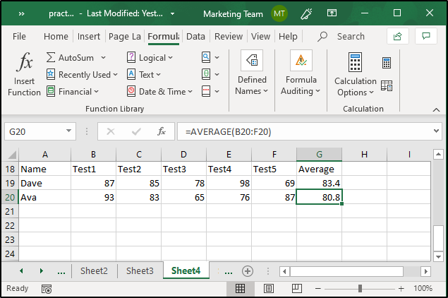
Average:
The average, as we all know, depicts the median value of a number of values. In Excel, the average can be easily calculated using the built-in function called “AVERAGE”. The syntax of this function is as follows:
AVERAGE(number1, number2, …)
EXAMPLE:
In case you want to calculate the average marks attained by students in all the exams, you can simply create a table and then use the AVERAGE formula to calculate the average marks attained by each student.
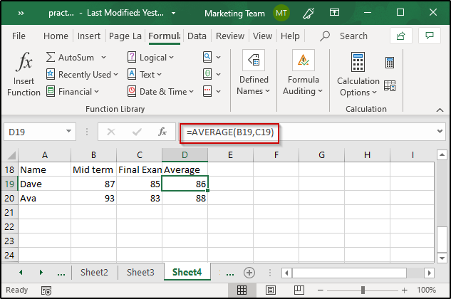
In the above example, I have calculated the average marks for two students in two exams. In case you have more than two values whose average needs to be determined, you just have to specify the range of cells wherein the values are present. For example:
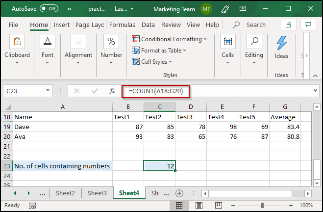
COUNT:
The count function in Excel will count the number of cells containing numbers in a given range. The syntax of this function is as follows:
COUNT(value1, value2, …)
EXAMPLE:
In case I want to calculate the number of cells holding numbers from the table I created in the previous example, I will simply have to select the cell wherein I want to display the result and then make use of the COUNT function as follows:
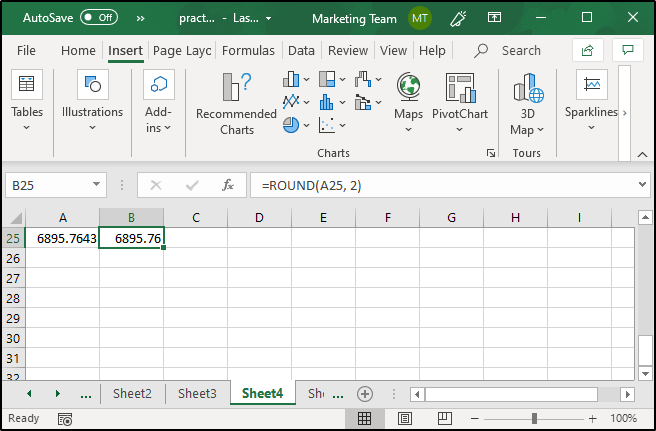
ROUND:
In order to round off values to some specific decimal places, you can make use of the ROUND function. This function will return a number by rounding it off to the specified number of decimal places. The syntax of this function is as follows:
ROUND(number, num_digits)
EXAMPLE:
Finding Grade:
In order to find grades, you will have to make use of nested IF statements in Excel. For example, in the Average example, I had calculated the average marks scored by students in the tests. Now, to find the Grades attained by these students, I will have to create a nested IF function as follows:

As you can see, the average marks are present in column G. To calculate the grade, I have used a nested IF formula. The code is as follows:
=IF(G19>90,”A”,(IF(G19>75,”B”,IF(G19>60,”C”,IF(G19>40,”D”,”F”)))))
After doing this, you will just have to copy the formula to all the cells where you want to display the grades.
RANK:
In case you want to determine the Rank attained by the students of a class, you can make use of one of the built-in Excel Formulas i.e RANK. This function will return the Rank for a specified range by comparing a given range in the ascending or in the descending order. The syntax of this function is as follows:
RANK(ref, number, order)
EXAMPLE:
![]()
As you can see, in the above example, I have calculated the Rank of the students using the Rank function. Here, the first parameter is the average marks attained by each student and the array is the average attained by all other students of the class. I have not specified any order, therefore, the output will be determined in the descending order. For ascending order ranks, you will have to specify any nonzero value.
COUNTIF:
In order to count the cells based on some given condition, you can use one of the built-in Excel Formulas called “COUNTIF”. This function will return the number of cells that satisfy some condition in a given range. The syntax of this function is as follows:
COUNTIF(range, criteria)
EXAMPLE:
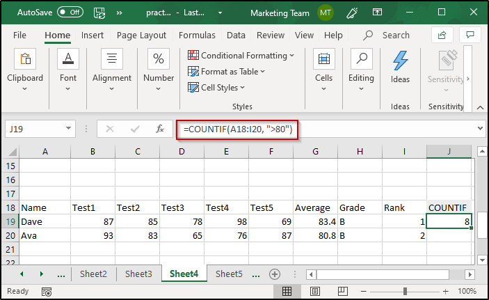
As you can see, in the above example, I have found the number of cells having values that are greater than 80. You can also give some text value to the criteria parameter.
INDEX:
The INDEX function returns a value or cell reference at some particular position in a specified range. The syntax of this function is as follows:
INDEX(array, row_num, column_num) or
INDEX(reference, row_num, column_num, area_num)
The index function works as follows for the Array form:
- If both row number and column number are supplied, it returns the value that is present at the intersection cell
- If the row value is set to zero, it will return the values present in the entire column in the specified range
- If the column value is set to zero, it will return the values present in the entire row in the specified range
The index function works as follows for the Reference form:
- Returns the reference of the cell where the row and the column values intersect
- The area_num will indicate which range is to be used in case multiple ranges have been supplied
EXAMPLE:
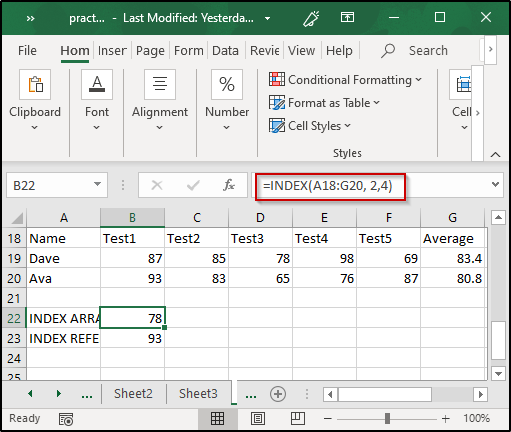
As you can see, in the above example, I have used the INDEX function to determine the value present in the 2nd row and 4th column for the range of cells between A18 to G20.
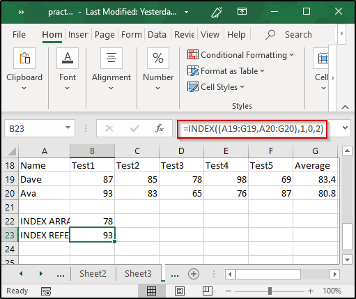
Similarly, you can also use the INDEX function by specifying multiple references as follows:
This brings us to the end of this article on Excel Formulas and Functions. I hope you are clear with all that has been shared with you. Make sure you practice as much as possible and revert your experience.
Got a question for us? Please mention it in the comments section of this “Excel Formulas and Functions” blog and we will get back to you as soon as possible.
To get in-depth knowledge on any trending technologies along with its various applications, you can enroll for live Edureka MS Excel Online training with 24/7 support and lifetime access.
Formulas and functions are the bread and butter of Excel. They drive almost everything interesting and useful you will ever do in a spreadsheet. This article introduces the basic concepts you need to know to be proficient with formulas in Excel. More examples here.
What is a formula?
A formula in Excel is an expression that returns a specific result. For example:
=1+2 // returns 3

=6/3 // returns 2

Note: all formulas in Excel must begin with an equals sign (=).
Cell references
In the examples above, values are «hardcoded». That means results won’t change unless you edit the formula again and change a value manually. Generally, this is considered bad form, because it hides information and makes it harder to maintain a spreadsheet.
Instead, use cell references so values can be changed at any time. In the screen below, C1 contains the following formula:
=A1+A2+A3 // returns 9

Notice because we are using cell references for A1, A2, and A3, these values can be changed at any time and C1 will still show an accurate result.
All formulas return a result
All formulas in Excel return a result, even when the result is an error. Below a formula is used to calculate percent change. The formula returns a correct result in D2 and D3, but returns a #DIV/0! error in D4, because B4 is empty:

There are different ways of handling errors. In this case, you could provide the missing value in B4, or «catch» the error with the IFERROR function and display a more friendly message (or nothing at all).
Copy and paste formulas
The beauty of cell references is that they automatically update when a formula is copied to a new location. This means you don’t need to enter the same basic formula again and again. In the screen below, the formula in E1 has been copied to the clipboard with Control + C:

Below: formula pasted to cell E2 with Control + V. Notice cell references have changed:

Same formula pasted to E3. Cell addresses are updated again:

Relative and absolute references
The cell references above are called relative references. This means the reference is relative to the cell it lives in. The formula in E1 above is:
=B1+C1+D1 // formula in E1
Literally, this means «cell 3 columns left «+ «cell 2 columns left» + «cell 1 column left». That’s why, when the formula is copied down to cell E2, it continues to work in the same way.
Relative references are extremely useful, but there are times when you don’t want a cell reference to change. A cell reference that won’t change when copied is called an absolute reference. To make a reference absolute, use the dollar symbol ($):
=A1 // relative reference
=$A$1 // absolute reference
For example, in the screen below, we want to multiply each value in column D by 10, which is entered in A1. By using an absolute reference for A1, we «lock» that reference so it won’t change when the formula is copied to E2 and E3:

Here are the final formulas in E1, E2, and E3:
=D1*$A$1 // formula in E1
=D2*$A$1 // formula in E2
=D3*$A$1 // formula in E3
Notice the reference to D1 updates when the formula is copied, but the reference to A1 never changes. Now we can easily change the value in A1, and all three formulas recalculate. Below the value in A1 has changed from 10 to 12:

This simple example also shows why it doesn’t make sense to hardcode values into a formula. By storing the value in A1 in one place, and referring to A1 with an absolute reference, the value can be changed at any time and all associated formulas will update instantly.
Tip: you can toggle between relative and absolute syntax with the F4 key.
How to enter a formula
To enter a formula:
- Select a cell
- Enter an equals sign (=)
- Type the formula, and press enter.
Instead of typing cell references, you can point and click, as seen below. Note references are color-coded:

All formulas in Excel must begin with an equals sign (=). No equals sign, no formula:

How to change a formula
To edit a formula, you have 3 options:
- Select the cell, edit in the formula bar
- Double-click the cell, edit directly
- Select the cell, press F2, edit directly
No matter which option you use, press Enter to confirm changes when done. If you want to cancel, and leave the formula unchanged, click the Escape key.
Video: 20 tips for entering formulas
What is a function?
Working in Excel, you will hear the words «formula» and «function» used frequently, sometimes interchangeably. They are closely related, but not exactly the same. Technically, a formula is any expression that begins with an equals sign (=).
A function, on the other hand, is a formula with a special name and purpose. In most cases, functions have names that reflect their intended use. For example, you probably know the SUM function already, which returns the sum of given references:
=SUM(1,2,3) // returns 6
=SUM(A1:A3) // returns A1+A2+A3
The AVERAGE function, as you would expect, returns the average of given references:
=AVERAGE(1,2,3) // returns 2
And the MIN and MAX functions return minimum and maximum values, respectively:
=MIN(1,2,3) // returns 1
=MAX(1,2,3) // returns 3
Excel contains hundreds of specific functions. To get started, see 101 Key Excel functions.
Function arguments
Most functions require inputs to return a result. These inputs are called «arguments». A function’s arguments appear after the function name, inside parentheses, separated by commas. All functions require a matching opening and closing parentheses (). The pattern looks like this:
=FUNCTIONNAME(argument1,argument2,argument3)
For example, the COUNTIF function counts cells that meet criteria, and takes two arguments, range and criteria:
=COUNTIF(range,criteria) // two arguments
In the screen below, range is A1:A5 and criteria is «red». The formula in C1 is:
=COUNTIF(A1:A5,"red") // returns 2

Video: How to use the COUNTIF function
Not all arguments are required. Arguments shown in square brackets are optional. For example, the YEARFRAC function returns fractional number of years between a start date and end date and takes 3 arguments:
=YEARFRAC(start_date,end_date,[basis])
Start_date and end_date are required arguments, basis is an optional argument. See below for an example of how to use YEARFRAC to calculate current age based on birthdate.
How to enter a function
If you know the name of the function, just start typing. Here are the steps:
1. Enter equals sign (=) and start typing. Excel will make a list of matching functions based as you type:

When you see the function you want in the list, use the arrow keys to select (or just keep typing).
2. Type the Tab key to accept a function. Excel will complete the function:

3. Fill in required arguments:

4. Press Enter to confirm formula:

Combining functions (nesting)
Many Excel formulas use more than one function, and functions can be «nested» inside each other. For example, below we have a birthdate in B1 and we want to calculate current age in B2:

The YEARFRAC function will calculate years with a start date and end date:

We can use B1 for start date, then use the TODAY function to supply the end date:

When we press Enter to confirm, we get current age based on today’s date:
=YEARFRAC(B1,TODAY())

Notice we are using the TODAY function to feed an end date to the YEARFRAC function. In other words, the TODAY function can be nested inside the YEARFRAC function to provide the end date argument. We can take the formula one step further and use the INT function to chop off the decimal value:
=INT(YEARFRAC(B1,TODAY()))

Here, the original YEARFRAC formula returns 20.4 to the INT function, and the INT function returns a final result of 20.
Notes:
- The current date in images above is February 22, 2019.
- Nested IF functions are a classic example of nesting functions.
- The TODAY function is a rare Excel function with no required arguments.
Key takeaway: The output of any formula or function can be fed directly into another formula or function.
Math Operators
The table below shows the standard math operators available in Excel:
| Symbol | Operation | Example |
|---|---|---|
| + | Addition | =2+3=5 |
| — | Subtraction | =9-2=7 |
| * | Multiplication | =6*7=42 |
| / | Division | =9/3=3 |
| ^ | Exponentiation | =4^2=16 |
| () | Parentheses | =(2+4)/3=2 |
Logical operators
Logical operators provide support for comparisons such as «greater than», «less than», etc. The logical operators available in Excel are shown in the table below:
| Operator | Meaning | Example |
|---|---|---|
| = | Equal to | =A1=10 |
| <> | Not equal to | =A1<>10 |
| > | Greater than | =A1>100 |
| < | Less than | =A1<100 |
| >= | Greater than or equal to | =A1>=75 |
| <= | Less than or equal to | =A1<=0 |
Video: How to build logical formulas
Order of operations
When solving a formula, Excel follows a sequence called «order of operations». First, any expressions in parentheses are evaluated. Next Excel will solve for any exponents. After exponents, Excel will perform multiplication and division, then addition and subtraction. If the formula involves concatenation, this will happen after standard math operations. Finally, Excel will evaluate logical operators, if present.
- Parentheses
- Exponents
- Multiplication and Division
- Addition and Subtraction
- Concatenation
- Logical operators
Tip: you can use the Evaluate feature to watch Excel solve formulas step-by-step.
Convert formulas to values
Sometimes you want to get rid of formulas, and leave only values in their place. The easiest way to do this in Excel is to copy the formula, then paste, using Paste Special > Values. This overwrites the formulas with the values they return. You can use a keyboard shortcut for pasting values, or use the Paste menu on the Home tab on the ribbon.
Video: Paste Special Shortcuts
What’s next?
Below are guides to help you learn more about Excel’s formulas and functions. We also offer online video training.
- 29 tips for working with formulas and functions (video version here)
- 500 formula examples with full explanations
- 101 important Excel functions
- Guide to all Excel functions (work in progress)
- Excel formula errors (examples and fixes)
- Formula criteria — 50 examples
- Formulas for conditional formatting
- How to use F9 to debug a formula (video)
- Excel formula errors and fixes (video)