What is format text in excel - Word и Excel - помощь в работе с программами

The TEXT function lets you change the way a number appears by applying formatting to it with format codes. It’s useful in situations where you want to display numbers in a more readable format, or you want to combine numbers with text or symbols.

Note: The TEXT function will convert numbers to text, which may make it difficult to reference in later calculations. It’s best to keep your original value in one cell, then use the TEXT function in another cell. Then, if you need to build other formulas, always reference the original value and not the TEXT function result.

Syntax

TEXT(value, format_text)

The TEXT function syntax has the following arguments:

Argument Name	Description
value	A numeric value that you want to be converted into text.
format_text	A text string that defines the formatting that you want to be applied to the supplied value.

Overview

In its simplest form, the TEXT function says:

=TEXT(Value you want to format, «Format code you want to apply»)

Here are some popular examples, which you can copy directly into Excel to experiment with on your own. Notice the format codes within quotation marks.

Formula	Description
=TEXT(1234.567,«$#,##0.00»)	Currency with a thousands separator and 2 decimals, like $1,234.57. Note that Excel rounds the value to 2 decimal places.
=TEXT(TODAY(),«MM/DD/YY»)	Today’s date in MM/DD/YY format, like 03/14/12
=TEXT(TODAY(),«DDDD»)	Today’s day of the week, like Monday
=TEXT(NOW(),«H:MM AM/PM»)	Current time, like 1:29 PM
=TEXT(0.285,«0.0%»)	Percentage, like 28.5%
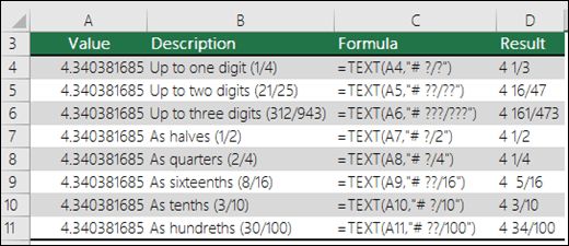
=TEXT(4.34 ,«# ?/?»)	Fraction, like 4 1/3
=TRIM(TEXT(0.34,«# ?/?»))	Fraction, like 1/3. Note this uses the TRIM function to remove the leading space with a decimal value.
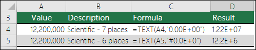
=TEXT(12200000,«0.00E+00»)	Scientific notation, like 1.22E+07
=TEXT(1234567898,«[<=9999999]###-####;(###) ###-####»)	Special (Phone number), like (123) 456-7898
=TEXT(1234,«0000000»)	Add leading zeros (0), like 0001234
=TEXT(123456,«##0° 00′ 00»»)	Custom — Latitude/Longitude

Note: Although you can use the TEXT function to change formatting, it’s not the only way. You can change the format without a formula by pressing CTRL+1 (or +1 on the Mac), then pick the format you want from the Format Cells > Number dialog.

Download our examples

You can download an example workbook with all of the TEXT function examples you’ll find in this article, plus some extras. You can follow along, or create your own TEXT function format codes.

Download Excel TEXT function examples

Other format codes that are available

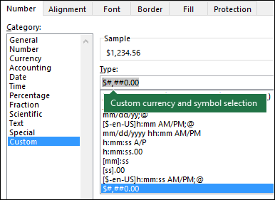
You can use the Format Cells dialog to find the other available format codes:

Press Ctrl+1 (+1 on the Mac) to bring up the Format Cells dialog.
Select the format you want from the Number tab.
Select the Custom option,
The format code you want is now shown in the Type box. In this case, select everything from the Type box except the semicolon (;) and @ symbol. In the example below, we selected and copied just mm/dd/yy.
Press Ctrl+C to copy the format code, then press Cancel to dismiss the Format Cells dialog.
Now, all you need to do is press Ctrl+V to paste the format code into your TEXT formula, like: =TEXT(B2,»mm/dd/yy«). Make sure that you paste the format code within quotes («format code»), otherwise Excel will throw an error message.

Format codes by category

Following are some examples of how you can apply different number formats to your values by using the Format Cells dialog, then use the Custom option to copy those format codes to your TEXT function.

Why does Excel delete my leading 0’s?

Excel is trained to look for numbers being entered in cells, not numbers that look like text, like part numbers or SKU’s. To retain leading zeros, format the input range as Text before you paste or enter values. Select the column, or range where you’ll be putting the values, then use CTRL+1 to bring up the Format > Cells dialog and on the Number tab select Text. Now Excel will keep your leading 0’s.

If you’ve already entered data and Excel has removed your leading 0’s, you can use the TEXT function to add them back. You can reference the top cell with the values and use =TEXT(value,»00000″), where the number of 0’s in the formula represents the total number of characters you want, then copy and paste to the rest of your range.

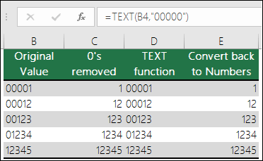
If for some reason you need to convert text values back to numbers you can multiply by 1, like =D4*1, or use the double-unary operator (—), like =—D4.

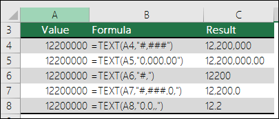
Excel separates thousands by commas if the format contains a comma (,) that is enclosed by number signs (#) or by zeros. For example, if the format string is «#,###», Excel displays the number 12200000 as 12,200,000.

A comma that follows a digit placeholder scales the number by 1,000. For example, if the format string is «#,###.0,», Excel displays the number 12200000 as 12,200.0.

Notes:

The thousands separator is dependent on your regional settings. In the US it’s a comma, but in other locales it might be a period (.).
The thousands separator is available for the number, currency and accounting formats.

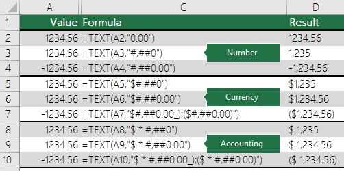
Following are examples of standard number (thousands separator and decimals only), currency and accounting formats. Currency format allows you to insert the currency symbol of your choice and aligns it next to your value, while accounting format will align the currency symbol to the left of the cell and the value to the right. Note the difference between the currency and accounting format codes below, where accounting uses an asterisk (*) to create separation between the symbol and the value.

To find the format code for a currency symbol, first press Ctrl+1 (or +1 on the Mac), select the format you want, then choose a symbol from the Symbol drop-down:

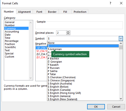
Then click Custom on the left from the Category section, and copy the format code, including the currency symbol.

Note: The TEXT function does not support color formatting, so if you copy a number format code from the Format Cells dialog that includes a color, like this: $#,##0.00_);[Red]($#,##0.00), the TEXT function will accept the format code, but it won’t display the color.

You can alter the way a date displays by using a mix of «M» for month, «D» for days, and «Y» for years.

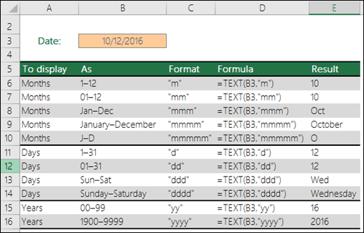
Format codes in the TEXT function aren’t case sensitive, so you can use either «M» or «m», «D» or «d», «Y» or «y».

You can alter the way time displays by using a mix of «H» for hours, «M» for minutes, or «S» for seconds, and «AM/PM» for a 12-hour clock.

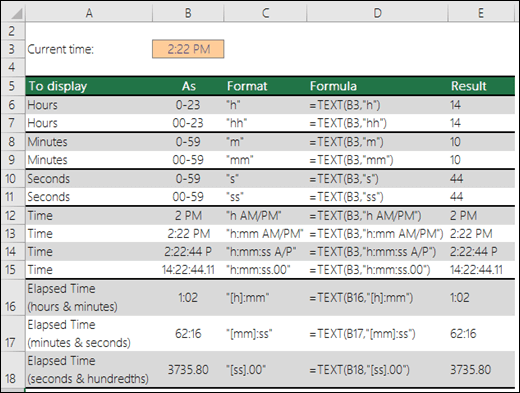
If you leave out the «AM/PM» or «A/P», then time will display based on a 24-hour clock.

Format codes in the TEXT function aren’t case sensitive, so you can use either «H» or «h», «M» or «m», «S» or «s», «AM/PM» or «am/pm».

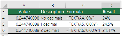
You can alter the way decimal values display with percentage (%) formats.

You can alter the way decimal values display with fraction (?/?) formats.

Scientific notation is a way of displaying numbers in terms of a decimal between 1 and 10, multiplied by a power of 10. It is often used to shorten the way that large numbers display.

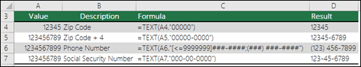
Excel provides 4 special formats:

Zip Code — «00000»
Zip Code + 4 — «00000-0000»
Phone Number — «[<=9999999]###-####;(###) ###-####»
Social Security Number — «000-00-0000»

Special formats will be different depending on locale, but if there aren’t any special formats for your locale, or if these don’t meet your needs then you can create your own through the Format Cells > Custom dialog.

Common scenario

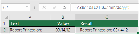
The TEXT function is rarely used by itself, and is most often used in conjunction with something else. Let’s say you want to combine text and a number value, like “Report Printed on: 03/14/12”, or “Weekly Revenue: $66,348.72”. You could type that into Excel manually, but that defeats the purpose of having Excel do it for you. Unfortunately, when you combine text and formatted numbers, like dates, times, currency, etc., Excel doesn’t know how you want to display them, so it drops the number formatting. This is where the TEXT function is invaluable, because it allows you to force Excel to format the values the way you want by using a format code, like «MM/DD/YY» for date format.

In the following example, you’ll see what happens if you try to join text and a number without using the TEXT function. In this case, we’re using the ampersand (&) to concatenate a text string, a space (» «), and a value with =A2&» «&B2.

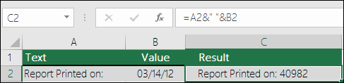
As you can see, Excel removed the formatting from the date in cell B2. In the next example, you’ll see how the TEXT function lets you apply the format you want.

Our updated formula is:

Cell C2:=A2&» «&TEXT(B2,»mm/dd/yy») — Date format

Frequently Asked Questions

Yes, you can use the UPPER, LOWER and PROPER functions. For example, =UPPER(«hello») would return «HELLO».

Yes, but it takes a few steps. First, select the cell or cells where you want this to happen and use Ctrl+1 to bring up the Format > Cells dialog, then Alignment > Text control > check the Wrap Text option. Next, adjust your completed TEXT function to include the ASCII function CHAR(10) where you want the line break. You might need to adjust your column width depending on how the final result aligns.

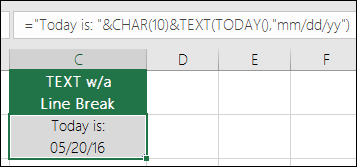
In this case, we used: =»Today is: «&CHAR(10)&TEXT(TODAY(),»mm/dd/yy»)

This is called Scientific Notation, and Excel will automatically convert numbers longer than 12 digits if a cell(s) is formatted as General, and 15 digits if a cell(s) is formatted as a Number. If you need to enter long numeric strings, but don’t want them converted, then format the cells in question as Text before you input or paste your values into Excel.

Introduction to Formatting Text in Excel

Excel has a wide range of variety for text formatting, which can make your results, dashboards, spreadsheets, an analysis that you do on day to day basis look fancier and attractive at the same time. Text formatting in Excel works in the same way as it does in other Microsoft tools such as Word and PowerPoint. This includes changing Font, Font Size, Font Color, Font Attribute (Such as making text, Bold, Italic, Underlined, etc.), text alignment, background color change, etc. This article will cover these text formatting tools in Excel along with examples for better understanding. Basically, all text formatting can be divided into two major groups, which are Font and Alignment. Each group has a variety of options using which we can format the text values and has its own relevance. e.g. within Font, you can have all the options associated with text fonts.

Please find attached is the screenshot for your reference:

Text Formatting Tools

All these text formatting tools are placed under the home tab. I am not considering the Clipboard in it because most of its part contains the cut, copy, paste, and Format Painter. Let’s start with Font and its options.

You can download this Formatting Text Excel Template here – Formatting Text Excel Template

1. Text Font

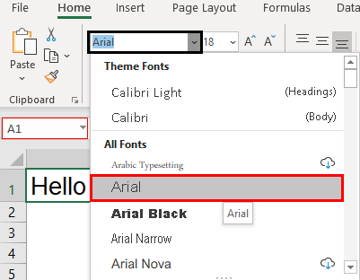
The first thing that comes into the picture when we talk about text formatting is Text Font. The default text font in Excel is set as Calibri (Body). However, it can be changed to any of the variety available in the fonts section.

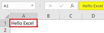
Let’s add some text under cell A1 of the Excel sheet.

As can be seen through the screenshot above, we have added as text “Hello World!” under cell A1 of the Excel sheet.

Navigate towards the Font section, where the default value is set as Calibri. Click on the dropdown menu, and you can see multiple fonts in which you can use for the text in cell A1. Choose anyone of your choice; I will use the Arial Black.

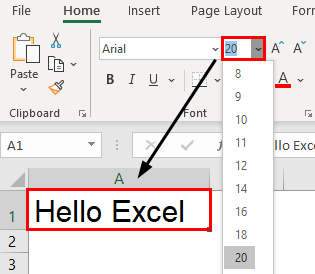
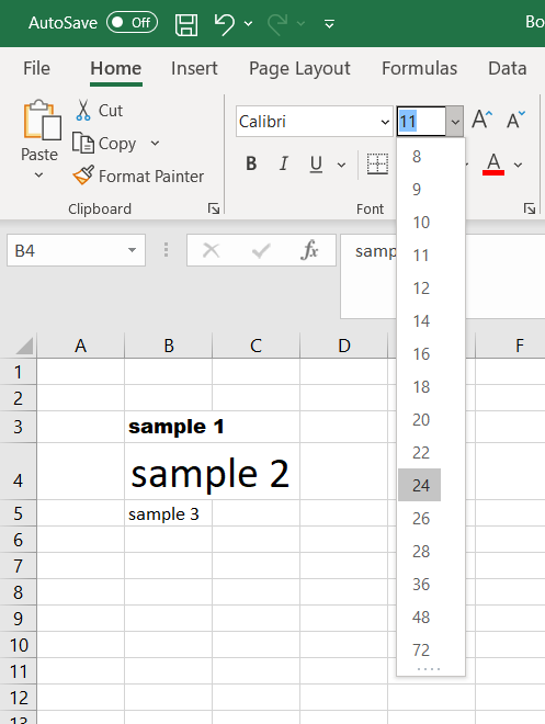
Now, we will try to change the font size.

Select the cell containing text (A1 in our example) and navigate towards the Font Size dropdown placed besides the Font option. Click on the dropdown, and you can see different font sizes starting from as low as 8. I will change the font size to 16. Please see the screenshot below for your reference.

You can also increase or decrease the font size using the Increase Font Size and Decrease Font Size buttons, which are placed right beside the Font Size dropdown. See the screenshot below:

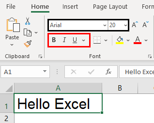
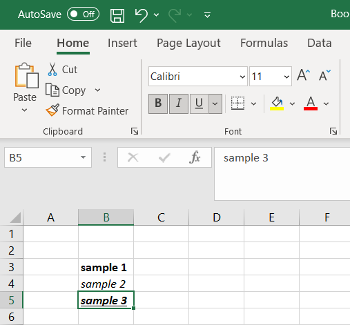
The next part comes when we have to change the text appearance. This covers the Bold, Italic, underlined text as well as coloring the text and/or cell containing the same.

Select the cell containing text and click on the bold button. It will make the text appear in bold. You can also achieve this by hitting Ctrl + B keys.

Select the cell and click on the Italic button that converts the text into Italic font. This can be achieved through a keyboard shortcut Ctrl + I.

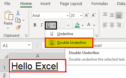
You can underline the text by using the Underline button that is placed besides the Italic button; the keyboard shortcut to achieve this result is Ctrl + U. There is one more option for the underlined section, and it is Double Underline. It adds a double underline to the current cell containing text. See the screenshot below for better visualization of these two options.

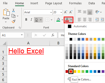
We also have an option to change the text color for a given text. This option is placed under the Font section in your excel ribbon. You can simply click on the change color dropdown and see different colors to add for the current text value. See the screenshot below for your reference:

This is how we can format the text using the Font Group. Now we will move towards the second group called Alignment.

2. Text Alignment

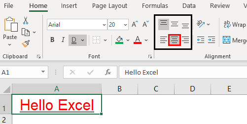
This part also plays an important role in text formatting. We have several alignment options available under this Group. We will see that one by one. Text alignment is of 6 types in total. The first three are Top Align, Middle Align, and Bottom Align. These are placed at the top most tier under the Alignment group.

Exactly below to these three, there are three more alignment options. Align Left, Center and Align Right. They are placed in the second tier of the options under the Alignment group.

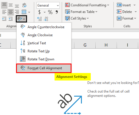
The third part that gets covered under the Alignment group is the Text Rotation option. This option has different text rotation options available, allowing you to rotate the text with angles (clockwise)and vertically (up and Down). This feature is rarely used though sometimes it is really helpful when you want to do something different with the headings of your reports.

Forth thing that gets covered under the Alignment section is the indentation. Most of us fail to recognize when to add or decrease an indentation. However, you don’t need to keep it in your mind. Excel has Increase Indent and Decrease Indent option that helps you either increase or decrease the indent in your current text.

The fifth and last thing that comes under alignment is Wrap Text and Merge& Center option. Well, these two are the most commonly used alignment operations in Excel. Wrap Text shows text in one single cell even if that text goes beyond the cell boundaries. On the other hand, Merge & Center merges the data across the multiple cells and then makes a centered alignment for the merged text. If you click on Merge & Center button again, it removes the effect; however, the text gets filled in the left most cell or a cell under which it has actually been entered.

The above screenshot emphasizes the use of Wrap Text. The actual text under A1 is beyond the cell boundary. However, with it having wrapped, it is under the cell boundary.

This screenshot emphasizes the use of Merge and Center. Instead of wrapping the text under same cell, we have tried it to merge across three cells A3:C3 and it looks nicer than before. This is how Merge & Center works.

This is how we can format the text under Excel. Now let’s wrap things up with some points to be remembered about Text Formatting in Excel.

Things to Remember

Font and Alignment covers most of the Text Formatting options under Excel
Some of the users also consider Conditional Formatting as a part of Text Formatting. It sometimes can be used to format the text. However, it is not dedicated to text formatting (We can also use conditional formatting on numbers).
You can use the Format Painter option under Clipboard to copy the text format and apply it to some other text in some other cell or sheet.

How to Format Text in Excel?

Formatting text in Excel includes color, font name, font size, alignment, font appearance in bold, underline, italic, background color of the font cell, etc.

How to Format Text in Excel?
- #1 Text Name
- #2 Font Size
- #3 Text Appearance
- #4 Text Color
- #5 Text Alignment
- #6 Text Orientation
- #7 Conditional Text Formatting
  - #1 – Highlight Specific Value
  - #2 – Highlight Duplicate Value
  - #3 – Highlight Unique Value
- Things to Remember
- Recommended Articles

You can download this Formatting Text Excel Template here – Formatting Text Excel Template

#1 Text Name

We can format the text font from default to any other available fonts in Excel. Likewise, we can insert any text value in any of the cells.

Under the “Home” tab, we can see so many formatting options available.

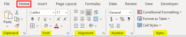
Formatting has been categorized into six groups: “Clipboard,” “Font,” “Alignment,” “Number,” and “Styles.”

In this, we are formatting the font of cell value A1, “Hello Excel.” For this, under the “Font” category, click on the “Font Name” drop-down list and select the font name as per wish.

We hover over one of the font names above. We can see the quick preview in cell A1. If you are satisfied with the font style, click on the name to fix the font name for the selected cell value.

#2 Font Size

Similarly, we can also format the font size of the text in a cell. Just type the font size in numbers next to the font name option.

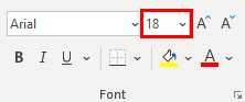
Enter the font size in numbers to see the impact.

#3 Text Appearance

We can modify the default view of the text value. For example, we can make the text value look bold, italic, and underlined. Look at font size and name options. We can see all these three options.

As per the format, we can apply formatting to text value.

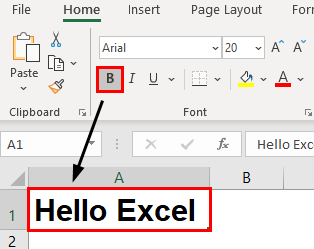
We have applied the “Bold” formatting using the Ctrl + B shortcut excel keyAn Excel shortcut is a technique of performing a manual task in a quicker way.read more.

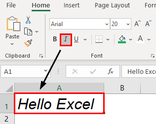
To apply “Italic” formatting, use the Ctrl + I shortcut key.

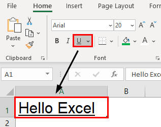
To apply “Underline” formatting, use the Ctrl + U shortcut key.

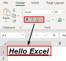
The below image shows a combination of all the above three options.

If we want to apply a double underline, click on the drop-down list of underline options and choose “Double Underline.”

#4 Text Color

We can format the default font color (black) of text to any colors available.

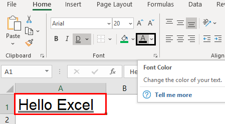
Click on the drop-down list of the “Font Color” option and change as per choice.

#5 Text Alignment

We can format the alignment of the Excel text under the “Alignment” group.

We can do a left alignment, right alignment, middle alignment, top alignment, and bottom alignment.

#6 Text Orientation

The important thing under “Alignment” is the “Orientation” of the text value.

Under “Orientation,” we can rotate text values diagonally or vertically.

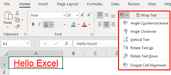
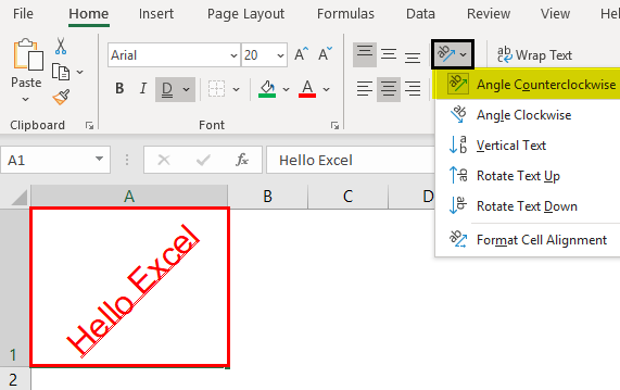
Angle Counterclockwise

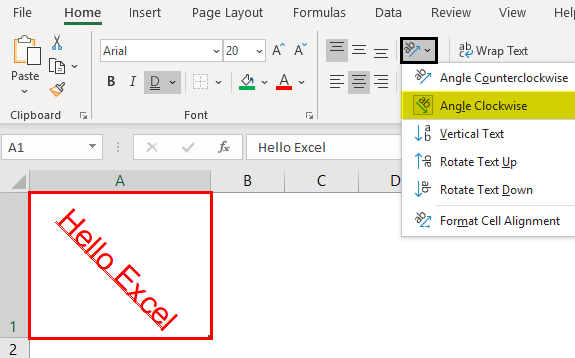
Angle Clockwise

Vertical Text

Rotate Text Up

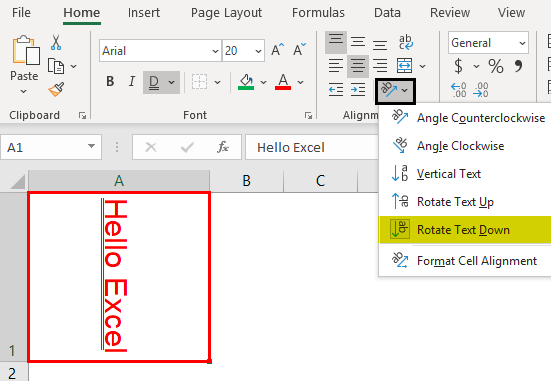
Rotate Text Down

Under “Format Cell Alignment, we have many options. Click on this option and experiment with some techniques to see the impact.

#7 Conditional Text Formatting

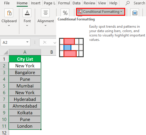
Let us see how to apply conditional formattingConditional formatting is a technique in Excel that allows us to format cells in a worksheet based on certain conditions. It can be found in the styles section of the Home tab.read more to text in Excel.

We have learned some of the basic text formatting techniques. How about the idea of formatting only a specific set of values from the group? If we want to find only duplicate values or find unique values.

These are possible through the conditional formatting technique.

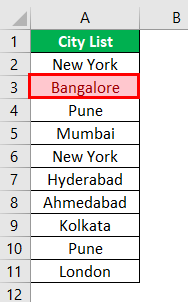
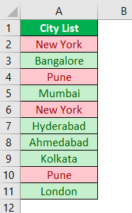
For example, look at the below list of cities.

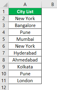
From this list, let us learn some formatting techniques.

#1 – Highlight Specific Value

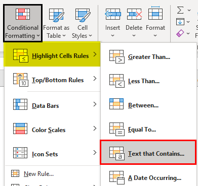
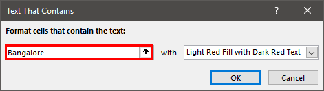
If we want to highlight only the specific city name, we can only highlight specific city names. For example, assume we want to highlight the city “Bangalore,” then select the data and go to conditional formatting.

Click on the drop-down list in excelA drop-down list in excel is a pre-defined list of inputs that allows users to select an option.read more of “Conditional Formatting” >>> “Highlight cells Rules” >>> “Text that Contains.”

Now, we will see the below window.

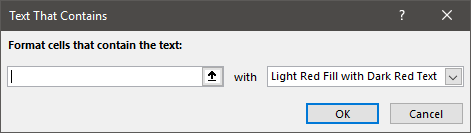
Next, we must enter the text value that we need to highlight.

Now from the drop-down list, we must choose the formatting style.

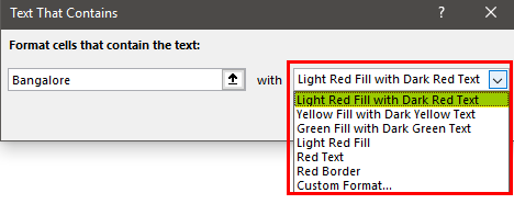
Click on “OK.” Consequently, it will highlight only the supplied text value.

#2 – Highlight Duplicate Value

To highlight duplicate values in excelHighlight Cells Rule, which is available under Conditional Formatting under the Home menu tab, can be used to highlight duplicate values in the selected dataset, whether it is a column or row of a table.read more, follow the below path.

“Conditional Formatting” >>> “Highlight cells Rules” >>> “Duplicate Values.”

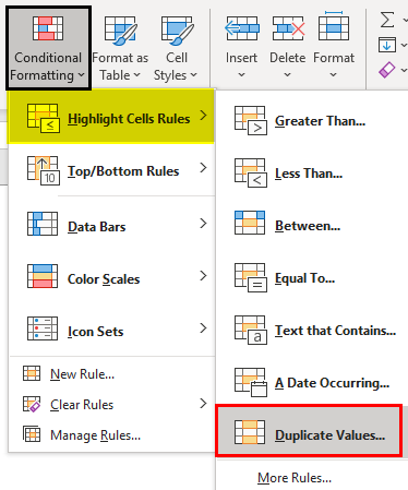
Again from the below window, we must select the formatting style.

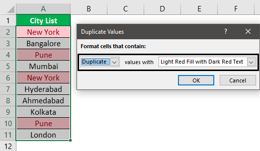
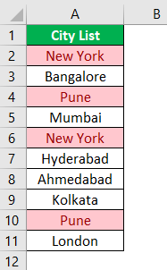
As a result, it will highlight only the text values that appear more than once.

#3 – Highlight Unique Value

Like how we have highlighted duplicate values similarly, we can highlight all the unique values, i.e., text value that appears only once. Then, the formatting window chooses the “Unique” value option from the duplicate values.

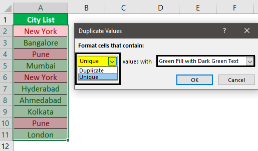
It will highlight only the unique values.

Things to Remember

We must learn shortcut keys to format text values in Excel quickly.
We can use conditional formatting to format some text values based on certain conditions.

Where is text or formatting in Excel?

If you want to search for text or numbers with specific formatting, click Format, and then make your selections in the Find Format dialog box. Tip: If you want to find cells that just match a specific format, you can delete any criteria in the Find what box, and then select a specific cell format as an example.

How do I format text in an Excel cell?

Tips & Tricks

Select the cell which you want to format.
In the formula bar highlight the part of the text that you want to format.
Go to the Home tab in the ribbon.
Press the dialog box launcher in the Font section.
Select any formatting options you want.
Press the OK button.

Is a text formatting?

Formatted text is text that is displayed in a special, specified style. … Text formatting data may be qualitative (e.g., font family), or quantitative (e.g., font size, or color). It may also indicate a style of emphasis (e.g., boldface, or italics), or a style of notation (e.g., strikethrough, or superscript).

What are the 4 types of formatting?

To help understand Microsoft Word formatting, let’s look at the four types of formatting:

Character or Font Formatting.
Paragraph Formatting.
Document or Page Formatting.
Section Formatting.

29 related questions found

What is an example of formatting?

The definition of a format is an arrangement or plan for something written, printed or recorded. An example of format is how text and images are arranged on a website. … They formatted the conference so that each speaker had less than 15 minutes to deliver a paper.

How do I format Excel cells to fit text?

Adjust text to fit within an Excel cell

Select the cell with text that’s too long to fully display, and press [Ctrl]1.
In the Format Cells dialog box, select the Shrink To Fit check box on the Alignment tab, and click OK.

What is the shortcut for text format in Excel?

To use the keyboard shortcuts:

Select the cell(s) you want to apply formatting to.
Press the keyboard shortcut by pressing and holding the keys in the following order: Ctrl + Shift + A (or the key you designate in the setup)
The cell formatting will be applied. You can use the Ctrl+Z or the Undo button to undo.

How do I see formatting in Excel?

How to Find and Replace Formatting in Excel

Click the Find & Select button on the Home tab.
Select Replace. …
Click the Options button.
Click the Find what: Format button. …
Select the formatting you want to find.
Click OK.
Click the Replace with: Format button.
Select the new formatting options you want to use.

How do you clear formatting in Excel?

Clear Formatting

Highlight the portion of the spreadsheet from which you want to remove formatting. Click the Home tab. Select Clear from the Editing portion of the Home tab. From the drop down menu of the Clear button, select Clear Formats.

How can I tell if a cell contains text?

Follow these steps to locate cells containing specific text:

Select the range of cells that you want to search. …
On the Home tab, in the Editing group, click Find & Select, and then click Find.
In the Find what box, enter the text—or numbers—that you need to find.

What is the shortcut key to apply bold formatting?

Select the text that you want to make bold, and do one of the following:

Move your pointer to the Mini toolbar above your selection and click Bold .
Click Bold in the Font group on the Home tab.
Type the keyboard shortcut: CTRL+B.

Which applies or removes bold formatting?

Ctrl + B Apply or remove bold format.

How do I apply text number format in Excel?

Format numbers as text

Select the cell or range of cells that contains the numbers that you want to format as text. How to select cells or a range. …
On the Home tab, in the Number group, click the arrow next to the Number Format box, and then click Text.

Can you format text in a cell in Excel?

Text formatting within a cell in Microsoft Excel works very much like it does in Word and PowerPoint. You can change the font, font size, color, attributes (such as bold or italic) and more for an Excel spreadsheet cell or range. Select the cell(s). … You can use the controls on the Home tab to work with cell alignment.

How do I convert text to number format in Excel?

Convert Text to Numbers Using ‘Convert to Number’ Option

Select all the cells that you want to convert from text to numbers.
Click on the yellow diamond shape icon that appears at the top right. From the menu that appears, select ‘Convert to Number’ option.

How do you AutoFit cell size to contents?

Automatically adjust your table or columns to fit the size of your content by using the AutoFit button.

Select your table.
On the Layout tab, in the Cell Size group, click AutoFit.
Do one of the following. To adjust column width automatically, click AutoFit Contents.

How do you make text fit in sheets?

Here’s how.

Select one or more cells containing the text you want to wrap. Select a header to highlight an entire row or column. …
Go to the Format menu.
Select the Text wrapping option to open a submenu containing three options: …
The cell enlarges to fit the text.

What are the three types of formatting?

To help understand Microsoft Word formatting, let’s look at the four types of formatting:

Character or Font Formatting.
Paragraph Formatting.
Document or Page Formatting.
Section Formatting.

What is formatting explain with example?

Format or document format is the overall layout of a document or spreadsheet. For example, the formatting of text on many English documents is aligned to the left of a page. With text, a user could change its format to bold to help emphasize text.

What is the formatting style?

Each formatting style is a set of predefined formatting options: (font size, color, line spacing, alignment etc.). … Applying a style depends on whether this style is a paragraph style (normal, no spacing, headings, list paragraph etc.), or a text style (based on the font type, size, color).

Which function key is used for style formatting?

The Shortcut Key used for opening Styles and Formatting Window is F11. F11 is shortcut key used for Opening or closing the Styles and Formatting window.

Источник

Changing the appearance of the text in a spreadsheet can make it easier to read. But how do you adjust the font, size and colour of the text? And how do you apply effects? In this article, we provide a quick guide to formatting text in Microsoft Excel.

How to Adjust Fonts in Excel

To change the font used in a cell in Microsoft Excel, you will need to:

Select all of the cells that you wish to format with the cursor.
Go to the Home tab on the main ribbon.
Click the fonts dropdown (i.e. the menu with the name of the current font in it).
Select the font you want to use from the list.

This will automatically change the typeface for any text already in the selected cell(s), plus any text later typed into the formatted cell(s).

Choosing the font from the drop-down list.

Changing the Font Size in Excel

To change the font size in Microsoft Excel, all you need to do is:

Select the cell(s) you want to format with the cursor.
Click the font size dropdown on the Home tab of the ribbon (i.e. the dropdown next to the main font menu).
Select a value from the list to adjust the size of the text in the selected cell(s).

You can also increase or decrease the font size by one step via the capital ‘A’ buttons with up and down arrows next to this dropdown.

Selecting a font size.

Changing the Font Colour in Excel

To change the font colour in Microsoft Excel:

Select the cell(s) you want to format.
Click the font colour button on the Home tab (see below).
Select a colour from the options available (or click More Colors… at the bottom of this menu to open a new pop-up with custom colours).

You can also change the background colour of a cell by using the Fill Color option to the left of the font colour menu (i.e. the paint bucket icon).

The font colour options in Microsoft Excel, accessed via the button in the bottom right of the font group.

Adjusting the font colour.

How to Apply Effects in Excel

In Excel, you can also apply italics, bold, and underlining to text. These effects can all be found next to each other in the font group of the Home tab.

Find this useful?

Subscribe to our newsletter and get writing tips from our editors straight to your inbox.

Bold, italics and underlining.

To apply your preferred style(s), select the cell(s) you wish to change, and then click on the B for bold, I for italics or U for underlining.

You also add strikethrough, subscript or superscript to text in Excel.

To do this, click the arrow in the bottom right of the font group to open the Format Cells pop-up. Make sure the Font tab is selected, then select your required formatting from the options in the Effects section of the window.

Adding effects to a cell.

You can make changes to the font, font size and font colour from this pop-up window too, if required, though it is usually quicker to do it via the Home tab.

Formatting Part of a Cell

Finally, what if you want to format a specific part of the text within a cell rather than all the text in a cell? Here’s how you do this:

Select the cell with the text you want to format.
In the formula bar, select the specific text you would like to change.
Choose your preferred formatting using the options set out above.

Changing part of the text in a cell.

The change will then be applied in the selected cell, but not in the formula bar.

Expert Spreadsheet Proofreading

Hopefully, this post has explained some of the basics of formatting text in Excel. But you’ll also want the text in your spreadsheets to be error-free. Why not send in a document today and have it checked by our spreadsheet experts?

Источник

Overview

Download our examples

Other format codes that are available

Format codes by category

Common scenario

Frequently Asked Questions

See Also

Introduction to Formatting Text in Excel

Text Formatting Tools

1. Text Font

2. Text Alignment

Things to Remember

Recommended Articles

How to Format Text in Excel?

Table of contents

#1 Text Name

#2 Font Size

#3 Text Appearance

#4 Text Color

#5 Text Alignment

#6 Text Orientation

#7 Conditional Text Formatting

#1 – Highlight Specific Value

#2 – Highlight Duplicate Value

#3 – Highlight Unique Value

Things to Remember

Recommended Articles

Where is text or formatting in Excel?

How do I format text in an Excel cell?

Is a text formatting?

What are the 4 types of formatting?

What is an example of formatting?

How do I format Excel cells to fit text?

What is the shortcut for text format in Excel?

How do I see formatting in Excel?

How do you clear formatting in Excel?

How can I tell if a cell contains text?

What is the shortcut key to apply bold formatting?

Which applies or removes bold formatting?

How do I apply text number format in Excel?

Can you format text in a cell in Excel?

How do I convert text to number format in Excel?

How do you AutoFit cell size to contents?

How do you make text fit in sheets?

What are the three types of formatting?

What is formatting explain with example?

What is the formatting style?

Which function key is used for style formatting?

How to Adjust Fonts in Excel

Changing the Font Size in Excel

Changing the Font Colour in Excel

How to Apply Effects in Excel

Find this useful?

Formatting Part of a Cell

Expert Spreadsheet Proofreading