
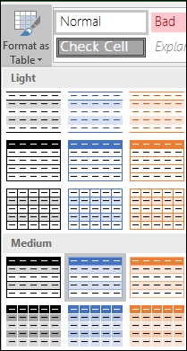
Excel provides numerous predefined table styles that you can use to quickly format a table. If the predefined table styles don’t meet your needs, you can create and apply a custom table style. Although you can delete only custom table styles, you can remove any predefined table style so that it is no longer applied to a table.

You can further adjust the table formatting by choosing Quick Styles options for table elements, such as Header and Total Rows, First and Last Columns, Banded Rows and Columns, as well as Auto Filtering.
Note: The screen shots in this article were taken in Excel 2016. If you have a different version your view might be slightly different, but unless otherwise noted, the functionality is the same.
Choose a table style
When you have a data range that is not formatted as a table, Excel will automatically convert it to a table when you select a table style. You can also change the format for an existing table by selecting a different format.
-
Select any cell within the table, or range of cells you want to format as a table.
-
On the Home tab, click Format as Table.

-
Click the table style that you want to use.
Notes:
-
Auto Preview — Excel will automatically format your data range or table with a preview of any style you select, but will only apply that style if you press Enter or click with the mouse to confirm it. You can scroll through the table formats with the mouse or your keyboard’s arrow keys.
-
When you use Format as Table, Excel automatically converts your data range to a table. If you don’t want to work with your data in a table, you can convert the table back to a regular range while keeping the table style formatting that you applied. For more information, see Convert an Excel table to a range of data.
Important:
-
Once created, custom table styles are available from the Table Styles gallery under the Custom section.
-
Custom table styles are only stored in the current workbook, and are not available in other workbooks.
Create a custom table style
-
Select any cell in the table you want to use to create a custom style.
-
On the Home tab, click Format as Table, or expand the Table Styles gallery from the Table Tools > Design tab (the Table tab on a Mac).
-
Click New Table Style, which will launch the New Table Style dialog.
-
In the Name box, type a name for the new table style.
-
In the Table Element box, do one of the following:
-
To format an element, click the element, then click Format, and then select the formatting options you want from the Font, Border or Fill tabs.
-
To remove existing formatting from an element, click the element, and then click Clear.
-
-
Under Preview, you can see how the formatting changes that you made affect the table.
-
To use the new table style as the default table style in the current workbook, select the Set as default table style for this document check box.

Delete a custom table style
-
Select any cell in the table from which you want to delete the custom table style.
-
On the Home tab, click Format as Table, or expand the Table Styles gallery from the Table Tools > Design tab (the Table tab on a Mac).
-
Under Custom, right-click the table style that you want to delete, and then click Delete on the shortcut menu.
Note: All tables in the current workbook that are using that table style will be displayed in the default table format.
-
Select any cell in the table from which you want to remove the current table style.
-
On the Home tab, click Format as Table, or expand the Table Styles gallery from the Table Tools > Design tab (the Table tab on a Mac).
-
Click Clear.
The table will be displayed in the default table format.
Note: Removing a table style does not remove the table. If you don’t want to work with your data in a table, you can convert the table to a regular range. For more information, see Convert an Excel table to a range of data.
There are several table style options that can be toggled on and off. To apply any of these options:
-
Select any cell in the table.
-
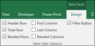
Go to Table Tools > Design, or the Table tab on a Mac, and in the Table Style Options group, check or uncheck any of the following:
-
Header Row — Apply or remove formatting from the first row in the table.
-
Total Row — Quickly add SUBTOTAL functions like SUM, AVERAGE, COUNT, MIN/MAX to your table from a drop-down selection. SUBTOTAL functions allow you to include or ignore hidden rows in calculations.
-
First Column — Apply or remove formatting from the first column in the table.
-
Last Column — Apply or remove formatting from the last column in the table.
-
Banded Rows — Display odd and even rows with alternating shading for ease of reading.
-
Banded Columns — Display odd and even columns with alternating shading for ease of reading.
-
Filter Button — Toggle AutoFilter on and off.
-
In Excel for the web, you can apply table style options to format the table elements.
Choose table style options to format the table elements
There are several table style options that can be toggled on and off. To apply any of these options:
-
Select any cell in the table.
-
On the Table Design tab, under Style Options, check or uncheck any of the following:
-
Header Row — Apply or remove formatting from the first row in the table.
-
Total Row — Quickly add SUBTOTAL functions like SUM, AVERAGE, COUNT, MIN/MAX to your table from a drop-down selection. SUBTOTAL functions allow you to include or ignore hidden rows in calculations.
-
Banded Rows — Display odd and even rows with alternating shading for ease of reading.
-
First Column — Apply or remove formatting from the first column in the table.
-
Last Column — Apply or remove formatting from the last column in the table.
-
Banded Columns — Display odd and even columns with alternating shading for ease of reading.
-
Filter Button — Toggle AutoFilter on and off.
-
Formatting cells as a table this is a process, that requires a lot of time, but that brings little benefit. A lot of effort can be saved by using ready-made styles of table layout.
Let`s descry ready-made designer stylish solutions that are predefined in the Excel tool set. You can also think about creating and maintaining your own styles. For this purpose, the program provides for special tools and tools.
How to create and format as a table in Excel?
We format the original range from the previous lessons with the helping of style design.
- Move the cursor to any cell in the table within the range A1:D4.
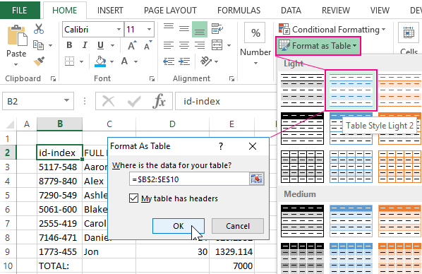
- Select the «Format as Table» tool on the «HOME» tab, the «Styles» section. There are the wide selection of ready-made and harmonious in design styles before you . Specify the style «Style Light 2». The dialog box appears where the range of the table data location is determined. Do not change anything, pressing OK.
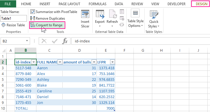
- The table has completely changed into a new and stylish format. There are even added filter control buttons. And on the broad band of tools the bookmark «DESIGN» was added, above which the inscription «TABLES TOOLS» is highlighted.
- To remove all unnecessary from our table and leave only the format, go to the «Designer» tab and in the «Tools» section, select «Convert to Range». Press OK to confirm.
The notation. Note, that Excel itself recognized to the size of the table, we did not need to allocate a range, it was enough to specify one of any cells.
Although there are a lot of styles, sometimes you can not find the right one. To save time, you should choose the most similar style and format it for your needs.
To clear the format, you must first select the required range of cells and select the tool on the «HOME tab» – «Editing» – «Clear Formats». For quick removal only of the cell boundaries, use the shortcut key combination CTRL + SHIFT + (minus). Just do not forget to select the range before that.
Try it!
- Select a cell within your data.
- Select Home > Format as Table.
- Choose a style for your table.
- In the Create Table dialog box, set your cell range.
- Mark if your table has headers.
- Select OK.
Contents
- 1 Why is format as table not working?
- 2 How do you convert a table format?
- 3 How do I convert text to a table in Excel?
- 4 How do I continue a Table format in Excel?
- 5 How do I extend a formatted Table in Excel?
- 6 How do I turn a table into a column in Excel?
- 7 How do I convert a table back to normal in Excel?
- 8 How do I edit a table in Excel?
- 9 How do you convert data into a Table?
- 10 How do I convert a text file to a Table?
- 11 How do I make a Table?
- 12 How do you create a format in Excel?
- 13 Why is my table not formatting in Excel?
- 14 How do you format data in Excel?
- 15 How do I create a dynamic table in Excel?
- 16 How do I create a multi column table in Excel?
- 17 How do I convert a table to a grid in Excel?
- 18 How do I copy a table into a cell in Excel?
- 19 How do you Deduplicate in Excel?
- 20 What is the quickest way to change the format of a table?
Why is format as table not working?
If applying table styles is not working, the range was probably already formatted before you converted it to a table. (Table formatting doesn’t override normal formatting.) To clear the existing background fill colors, select the entire table and choose Home> Font> Fill Color> No Fill.
How do you convert a table format?
Microsoft Word – Convert a Table to Text
- Select the rows or table you want to convert.
- Under the Table Tools tab, select the Layout tab.
- Select Convert to Text.
- Select what you want to separate the text with: Paragraph marks, Tabs, Commas, or Other.
- Select OK.
How do I convert text to a table in Excel?
Select the text that you want to convert, and then click Insert > Table > Convert Text to Table. In the Convert Text to Table box, choose the options you want. Under Table size, make sure the numbers match the numbers of columns and rows you want. In the Fixed column width box, type or select a value.
How do I continue a Table format in Excel?
On the Home tab, in the Styles group, click Format as Table. Click the table style that you want to use. Tips: Auto Preview – Excel will automatically format your data range or table with a preview of any style you select, but will only apply that style if you press Enter or click with the mouse to confirm it.
How do I extend a formatted Table in Excel?
Resize a table by adding or removing rows and columns
- Click anywhere in the table, and the Table Tools option appears.
- Click Design > Resize Table.
- Select the entire range of cells you want your table to include, starting with the upper-leftmost cell.
- When you’ve selected the range you want for your table, press OK.
How do I turn a table into a column in Excel?
Select the table you want to transform into a single column. Click on Copy on the left-hand side of the “Professor Excel”-ribbon. Select the first cell from which Professor Excel should paste the columns underneath. Click on “Paste to Single Column” on the “Professor Excel” ribbon.
How do I convert a table back to normal in Excel?
If you need to convert the table back to the normal data range, Excel also provides an easy way to deal with it.
- Select your table range, right click and select Table > Convert to Range from the context menu.
- Tip: You can also select the table range, and then click Design > Convert to Range.
How do I edit a table in Excel?
Modifying tables
- Select any cell in your table. The Design tab will appear on the Ribbon.
- From the Design tab, click the Resize Table command. Resize Table command.
- Directly on your spreadsheet, select the new range of cells you want your table to cover. You must select your original table cells as well.
- Click OK.
How do you convert data into a Table?
Convert Data Into a Table in Excel
- Open the Excel spreadsheet.
- Use your mouse to select the cells that contain the information for the table.
- Click the “Insert” tab > Locate the “Tables” group.
- Click “Table”.
- If you have column headings, check the box “My table has headers”.
How do I convert a text file to a Table?
How to Convert Text to a Table in Word
- Open the document you want to work in or create a new document.
- Select all the text in the document and then choose Insert→Table→Convert Text to Table. You can press Ctrl+A to select all the text in the document.
- Click OK.
- Save the changes to the document.
How do I make a Table?
For a basic table, click Insert > Table and move the cursor over the grid until you highlight the number of columns and rows you want. For a larger table, or to customize a table, select Insert > Table > Insert Table.
How do you create a format in Excel?
Apply a custom number format
- Select the cell or range of cells that you want to format.
- On the Home tab, under Number, on the Number Format pop-up menu. , click Custom.
- In the Format Cells dialog box, under Category, click Custom.
- At the bottom of the Type list, select the built-in format that you just created.
- Click OK.
Why is my table not formatting in Excel?
The reason this happens is because the number formatting was NOT applied to all of the cells in the column at the same time. If you apply number formatting to one cell, then apply the same format to the rest of the cells in the column later, the Table does NOT set that as the formatting for the entire column.
How do you format data in Excel?
Formatting text and numbers
- Select the cells(s) you want to modify. Selecting a cell range.
- Click the drop-down arrow next to the Number Format command on the Home tab. The Number Formatting drop-down menu will appear.
- Select the desired formatting option.
- The selected cells will change to the new formatting style.
How do I create a dynamic table in Excel?
#1 – Using Tables to create Dynamic Tables in Excel
- Select the data, i.e., A1:E6.
- In the Insert tab, click on Tables under the tables section.
- A dialog box pops up.
- Our Dynamic Range is created.
- Select the data and in the Insert Tab under the excel tables section, click on pivot tables.
How do I create a multi column table in Excel?
How to combine two or more columns in Excel
- In Excel, click the “Insert” tab in the top menu bar.
- In the “Create Table” dialog box that pops up, edit the formula so that only the columns and rows that you want to combine are used in the table.
How do I convert a table to a grid in Excel?
Choose Cross table to list option under Transpose type. button under Source range to select the data range that you want to convert. button under Results range to select a cell where you want to put the result. With this utility, you also convert flat list table to 2-dimensional cross table.
How do I copy a table into a cell in Excel?
Copy a Word table into Excel
- In a Word document, select the rows and columns of the table that you want to copy to an Excel worksheet.
- To copy the selection, press CTRL+C.
- In the Excel worksheet, select the upper-left corner of the worksheet area where you want to paste the Word table.
- Press CRL+V.
How do you Deduplicate in Excel?
Remove duplicate values
- Select the range of cells that has duplicate values you want to remove. Tip: Remove any outlines or subtotals from your data before trying to remove duplicates.
- Click Data > Remove Duplicates, and then Under Columns, check or uncheck the columns where you want to remove the duplicates.
- Click OK.
What is the quickest way to change the format of a table?
If you don’t like the default table format, you can easily change it by selecting any of the inbuilt Table Styles on the Design tab. The Design tab is the starting point to work with Excel table styles. It appears under the Table Tools contextual tab, as soon as you click any cell within a table.
Back in Excel 2007, Tables were added. That simple name hides a quite different and powerful Excel option that, in our view, Microsoft hasn’t explained very well.
Excel is often used for lists and Excel Tables make managing and extending those lists a lot easier. In fact, ‘Excel Lists’ was the name of the Tables predecessor in Excel. Word and PowerPoint have a ‘Tables’ feature but that’s quite different from Excel Tables.
Versions
Excel Tables are in Excel 2007, 2010, 2013 and 2016 for Windows, though the exact features will have changed over the decade.
Tables are also in Excel 2016 for Mac and seem much the same as Office 2016 for Windows.
Format as Table
You’ve probably seen Tables because they have a prominent place on the Home tab.

The label ‘Format as Table’ and the pull-down gallery gives the notion that Excel Tables are all about appearance/formatting. Microsoft also gives this impression in their description of Tables.
More than just appearances
In this article we’ll show you what’s useful in Excel Tables. We’ll leave aside the styles and galleries to show you the real benefits of tables.
Before Excel Tables
To understand Tables, let’s look at Excel life before they existed. Lists in Excel were a simple set of columns and rows.

You could add some structure to the list by clicking the Home | Sort and Filter | Filter button.

That made Row 1 into headers and little pull-down menus with sort and filter options.

The big problem with this was naming and keeping the data together.
If you added new rows to the list, you had to change any references to include the new rows.
For example, any formulas or refences with range A1:D5 would have to be changed to A1:D6 when you added a row.
Defining a named range helped, but you still needed to redefine the range each time the list was changed.
Excel Tables largely solve the naming and expansion issues. They make list sorting and filtering better plus a whole lot more.
What makes Excel Tables different
Tables are automatically Excel objects that you can refer to in formulas etc. They are automatically given names, starting with ‘Table1’, shown on the left of the Table Tools | Design ribbon.

But you can and should change the name to something more obvious.
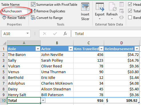
Right next to the Table Name is the important Resize Table option but you may not ever need it because of the vital Excel Table trick, Automatic Resizing.
Automatic Resizing
Excel Tables automatically expand when you add new rows to the bottom! It’s hard to underestimate the importance and usefulness of this seemingly simple addition.
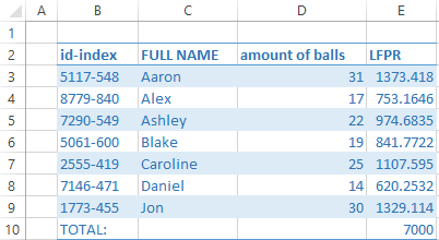
Here’s a simple example. A small table that we’ve formatted so the boundaries of the table are in blue outline.

Notice that the cells below the third entry (Vulcan) are NOT part of the table.
Now we start typing on the next line below the table and Lo! the table expands another row (see the blue boundary has dropped down a row). No change to the table settings is required, just typing another row is enough.

The same thing happens if you paste more rows to the bottom of the table.

Adding a column/field to a table just as simple. Here we’ve typed a new heading to the right of the existing headers.

As soon as Enter is pressed to complete the cell text, it becomes part of the Table.

Table Columns have names
Each column in a table has, in effect, a named range that you can use in formulas. They are officially called structured references because they have more options than normal Excel named ranges.
Use square brackets to signify the structured reference/range. Here’s the total, as a formula with [Kms Travelled] as the range to be totaled.
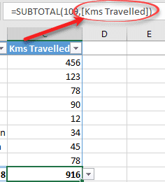
AutoComplete knows about these references, type an opening square bracket in a table formula and the list of possibles will appear.

Excel is pretty smart about using these names. If you select the data cells in a column, Excel will automatically use the name instead. Just like the table itself, the names will adjust when the table expands or contracts.
The names can be used outside the table itself, all you need to do is add the table name before the column name as in Munchausen[Kms Travelled]
Real Excel nerds can go crazy with the advanced naming options. You can use qualifiers like [#Headers] and [#All] to specify what you want use in the formula.
TableExample[[#Headers],[#Data],[Numbers]] will select both the Header and Data cells from the Numbers column in the table TableExample.
Confused?
Microsoft’s own explanation of an Excel Table is confusing, in fact quite circular.
“A table typically contains related data in a series of worksheet rows and columns that have been formatted as a table. ”
In other words, a table is a set of rows/columns formatted as a table. That doesn’t tell you anything. To put it another way:
“A house typically contains related rooms in a series of walls and floors that have been formatted as a house. “. Now you know that a house has rooms, walls and floors, but nothing more.
How to Format Tables in MS Excel
Now we will see how we can format tables in MS Excel.
For creating table we have an option in our HOME tab also so as ‘Format as
Table’, otherwise we can also use ‘Ctrl+T’ shortcut key for creating table.
To select all the data in our Excel sheet we will press ‘Ctrl+A’ shortcut
key, and then after to check that all our data is completely selected we
can press ‘Ctrl+.’ shortcut key to see on each corner cell of our data that
it is properly selected or not.
Now to convert the data into table format we will first select all the
data, and then click insert table in our INSERT tab, and hence table will
be created.
While creating table the only thing which you have to keep in mind is that
no row should be kept empty.
Also when our table will be created we will see a ‘Table tools’ option
above our DESIGN tab, which provide different styles and formats of table
like dark, medium, light etc..
We have also other option like banded rows in banded columns in MS Excel
which we can change according to our requirement from ‘Table tools’.
If you want to highlight first column or last column then we can select
their separate options which are already present in DESIGN column.
We have an option of ‘Total row’ which will give us a row at last which
will show the Total of our data which we have taken.
In table we have a very good functionality which is known as ‘Slicer’. It
is used to filter all the data of our table. When we use this option we can
see that some particular columns which we selected are shown in a dialogue
box in front of our screen. Then we can select any data which we want to be
displayed.