

Try it!
Use filters to temporarily hide some of the data in a table, so you can focus on the data you want to see.
Filter a range of data
-
Select any cell within the range.
-
Select Data > Filter.

-
Select the column header arrow
. -
Select Text Filters or Number Filters, and then select a comparison, like Between.
-
Enter the filter criteria and select OK.
Filter data in a table
When you Create and format tables, filter controls are automatically added to the table headers.

-
Select the column header arrow
for the column you want to filter. -
Uncheck (Select All) and select the boxes you want to show.
-
Click OK.
The column header arrow  changes to a
  Filter icon. Select this icon to change or clear the filter.
Want more?
Filter data in a range or table
Filter data in a PivotTable
Need more help?
Want more options?
Explore subscription benefits, browse training courses, learn how to secure your device, and more.
Communities help you ask and answer questions, give feedback, and hear from experts with rich knowledge.
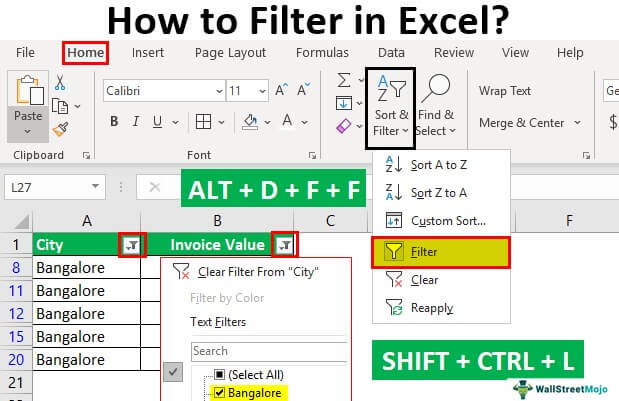
What is Filter in Excel?
The filter in excel helps display relevant data by eliminating the irrelevant entries temporarily from the view. The data is filtered as per the given criteria. The purpose of filtering is to focus on the crucial areas of a dataset. For example, the city-wise sales data of an organization can be filtered by the location. Hence, the user can view the sales of selected cities at a given time.
A filter is necessarily required when working with a huge database. Being a widely used tool, the filter converts a comprehensive view into an easy-to-understand one. To apply filters, the dataset must contain a header row which specifies the name of every column.
Table of contents
- What is Filter in Excel?
- How to Filter in Excel?
- Method 1: With Filter Option Under the Home tab
- Method 2: With Filter Option Under the Data tab
- Method 3: With the Shortcut key
- How to Add Filters in Excel?
- Example #1–“Number Filters” Option
- Example #2–“Search Box” Option
- Option while you Drop Down the Filter Function
- The Techniques of Filtering in Excel
- Frequently Asked Questions
- Recommended Articles
- How to Filter in Excel?
You are free to use this image on your website, templates, etc, Please provide us with an attribution linkArticle Link to be Hyperlinked
For eg:
Source: Filter in Excel (wallstreetmojo.com)
How to Filter in Excel?
You can download this Filter Column Excel Template here – Filter Column Excel Template
It is good to work with filters because they fit our needs the way we want to. In order to filter data, select the entries to be visible and deselect the rest of the items.
The three methods to add filters in excel are listed as follows:
- With filter option under the Home tab
- With filter option under the Data tab
- With the shortcut key
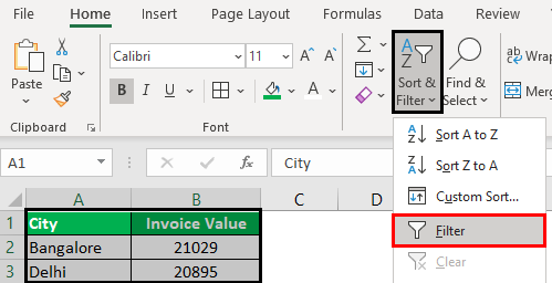
Let us consider a dataset to go through the three methods of adding filters.
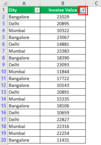
The following table shows the invoices issued to the buyers of different cities. We want to filter the data using different methods.

Method 1: With Filter Option Under the Home tab
In the Home tab, there is a “filter” option under the “sort and filter” drop-down of the “editing” section, as shown in the following image.
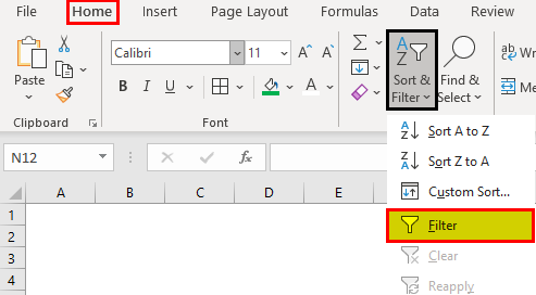
Step 1: Select the data and click “filter” under the “sort and filter” drop-down.
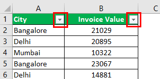
Step 2: The filters are added to the selected data range. The drop-down arrows, shown within the red boxes in the following image, are filters.
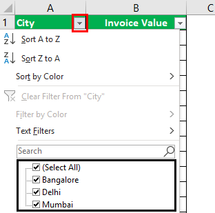
Step 3: Click the drop-down arrow of the column “city” to view the different names of the cities.
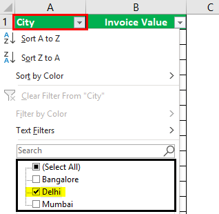
Step 4: To see the invoice values of “Delhi” only, select “Delhi” and uncheck all the remaining boxes.
Step 5: The data for the city “Delhi” is filtered and displayed in the following image.

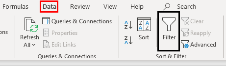
Method 2: With Filter Option Under the Data tab
In the Data tab, there is a “filter” option under the “sort and filter” section, as shown in the following image.
Method 3: With the Shortcut key
The keyboard shortcutsAn Excel shortcut is a technique of performing a manual task in a quicker way.read more are a good way to speed up the daily tasks. Select the data and add the filter using either of the following shortcuts:
- Press the keys “Shift+Ctrl+L” together.

- Press the keys “Alt+D+F+F” together.

Note: The preceding shortcuts for adding filtersUsing sorting and filtering, we can see the data category wise. With filtering data quickly you can easily navigate through menus or clicking through a mouse in less time.read more are toggle keys. Repetitive pressing helps to turn on and turn off the filters.
How to Add Filters in Excel?
We can filter numbers using advanced techniques. Let us consider some examples to understand the working of filters in Excel.
Example #1–“Number Filters” Option
Working on the data under the preceding heading (methods of filtering in Excel), we want to apply the following filters:
a. To filter column B (invoice value) for numbers greater than 10000
b. To filter column B for numbers greater than 10000 but less than 20000
Let us go through the two cases one by one.
a. Filter numbers greater than 10000
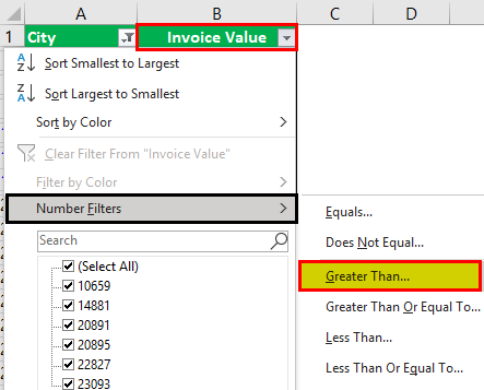
Step 1: Open the filter in column B (invoice value) by clicking on the filter symbol.
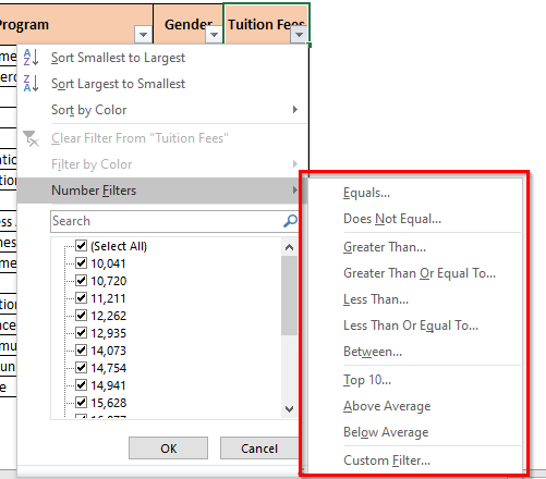
Step 2: In “number filters,” choose the “greater than” option, as shown in the following image.
Step 3: The “custom autofilter” box appears.
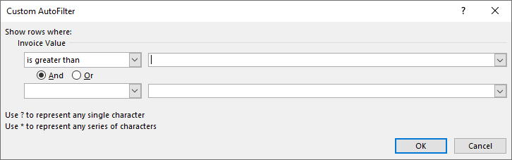
Step 4: Enter the number 10000 in the box to the right of “is greater than.”
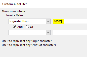
Step 5: The output displays the invoice values greater than 10000. The symbol within the red box is the filter icon. It indicates that the filter has been applied to column B.
b. Filter numbers greater than 10000 but less than 20000
Step 1: In “number filters,” choose the “greater than” option.
Step 2: In the “custom autofilter” box, select “is less than” in the second box to the left-hand side. This is shown in the following image.
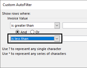
Step 3: Enter the number 10000 in the box to the right of “is greater than.” Enter the number 20000 in the box to the right of “is less than.”
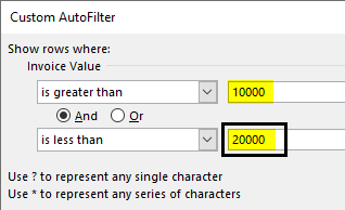
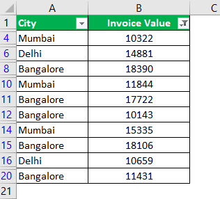
Step 4: The output displays the invoice values greater than 10000 but less than 20000.
Example #2–“Search Box” Option
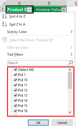
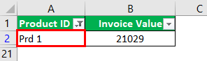
Working on the data under the preceding heading (methods of filtering in Excel), we have replaced the first column (city) with product IDs.
We want to filter the details of product ID “prd 1.”
The steps are listed as follows:
Step 1: Add filters to the columns “product ID” and “invoice value.”
Step 2: In the search boxA search box in Excel finds the needed data by typing into it, then filters the data and displays only that much info. When working with large datasheets, this simple tool may save a lot of time.read more, enter the value that is to be filtered. So, enter “prd 1.”
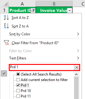
Step 3: The output displays only the filtered value from the list, as shown in the following image. Hence, we can see the invoice value of the product ID “prd 1.”
Option while you Drop Down the Filter Function
- Sort A to Z and Sort Z to A: If you wish to arrange your data ascending or descending order.
- Sort by Color: If you want to filter the data by color if a cell is filled by color.
- Text filter: When you want to filter a column with some exact text or number.
- Filter cells that begin with or end with an exact character or the text
- Filter cells that contain or do not contain a given character or word anywhere in the text.
- Filter cells that are exactly equal or not equal to a detailed character.
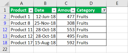
For example:
- Suppose you want to use the filter for a specific item. Click on to text filter and choose equals.
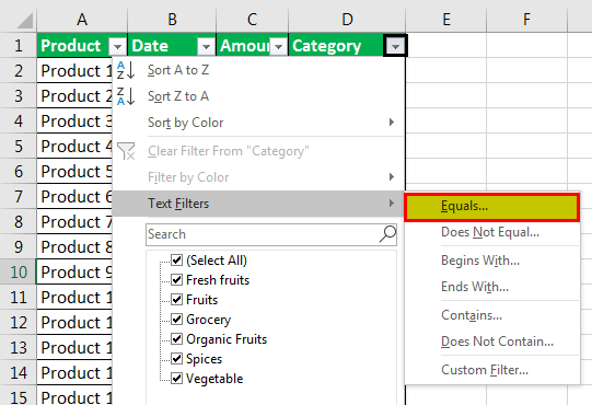
- It enables you the one dialogue, which includes a Custom Auto-Filter dialogue box.
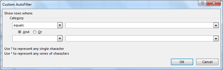
- Enter fruits under category and click Ok.
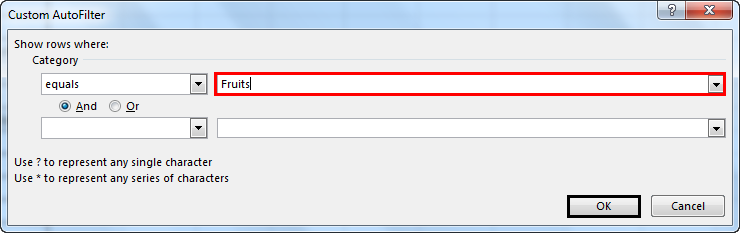
- Now you will get the data of fruits category only as shown below.
The Techniques of Filtering in Excel
The following techniques must be followed while filtering data:
- If the dataset is large, type the value to be filtered. This filters all the possible matches.
- If numerical data has to be filtered by specifying the greater than or the less than number, use the “number filters” option.
- If data has to be filtered by the color of specific rows, use the “filter by color” option.
Frequently Asked Questions
1. What are filters and how to add them in Excel?
Filtering is a technique which displays the required information and removes the unwanted data from the view. It helps the user focus on the relevant data at a given time.
The steps to add filters in Excel are listed as follows:
• Ensure that a header row appears on top of the data, specifying the column labels.
• Select the data on which filters are to be added.
• Add filters by any of the three given methods.
o Click the “filter” option under the “sort and filter” (editing section) drop-down of the Home tab.
o Click the “filter” option under the “sort and filter” section of the Data tab.
o Press the keys “Shift+Ctrl+L” or “Alt+D+F+F.”
Note: As soon as the filters are added, a drop-down arrow appears on the particular column header.
2. How to apply filters to one or more columns?
The steps to apply filters to one or more columns are listed as follows:
• Click the drop-down arrow of the column to be filtered.
• Uncheck the “select all” option which helps deselect all data.
• Select the boxes to be displayed.
• Click “Ok.”
The drop-down arrow changes to the filter icon as soon as a filter is applied. When filters are applied to multiple columns, the filter icon appears on each one of them. Hovering over the filter icon shows the filters that have been applied.
Note: The drop-down arrow on a column header indicates a filter is added. The filter icon indicates a filter has been applied.
3. How to use filters in Excel?
The filters can be applied to numbers, text values, and dates. These cases are discussed as follows:
Filter numbers
• Click on the “number filters.”
• Select any of the options like “equals,” “does not equals,” “greater than,” “less than,” “between,” “above average,” and so on.
• Specify the required fields in the dialog box that appears. This box may or may not be displayed.
For instance, in “equals,” enter the number against which the values should be compared. The filtered results show the matching numerical values.
Filter text and date values
• To filter text and date values, select “text filters” and “date filters” from the respective drop-down arrows.
• The “text filters” allow filtering text strings which contain specific characters or words. The “date filters” allow filtering dates for a particular year, month, week, and so on.
Note: The “plus” and the “minus” sign of the date filters are used for expanding and collapsing the various levels respectively.
Recommended Articles
This has been a guide to Filter in Excel. Here we discuss how to use/add filters in excel along with step by step examples and a downloadable template. You may learn more about Excel from the following articles –
- VBA FilterThe VBA Filter tool is used to sort out or fetch the desired data. However, this function accepts optional arguments, and the only required argument is an expression that covers the range, such as worksheets(«Sheet1»). Range(“A1”).read more
- How to Filter Pivot Table?By right-clicking on the pivot table, we can access the pivot table filter option. Another approach is to use the filter options available in the pivot table fields.read more
- Advanced Filter in ExcelThe advanced filter is different from the auto filter in Excel. This feature is not like a button that one can use with a single click of the mouse. To use an advanced filter, we have to define criteria for the auto filter and then click on the “Data” tab. Then, in the advanced section for the advanced filter, we will fill our criteria for the data.read more
- Types of Filters in Power BIThe filter function in Power BI is more commonly used to read data or reports based on multiple criteria. Visual level filters, page-level filters, report-level filters, drill-through filters, and so on are all available filters in Power Bi.read more
Filtering data in MS Excel refers to displaying only the rows that meet certain conditions. (The other rows gets hidden.) Using the store data, if you are interested in seeing data where Shoe Size is 36, then you can set filter to do this.
Contents
- 1 What is the purpose of filtering data?
- 2 What is Sorting and filtering Excel?
- 3 Why is filtering important in Excel?
- 4 What do you mean by filtering?
- 5 What is difference between filtering and sorting?
- 6 What is the difference between short and filter?
- 7 What is custom filtering?
- 8 When would you want to filter data in Excel?
- 9 What is filter give example?
- 10 What do you mean by filtering in computer?
- 11 What is filtering data in computer?
- 12 What is filter in computer class 10?
- 13 What do you mean by filtering data Class 10?
- 14 What is the difference between sieving from filtering?
- 15 What are the advantages of sorting and filtering data?
- 16 How do I copy filtered data in Excel?
- 17 What is the difference between filtering data by selection and filtering data by form?
- 18 What are steps to filter data in a table?
- 19 What is Result Filter in MVC?
- 20 What is custom filtering give one example?
What is the purpose of filtering data?
Filtering Data
When data is filtered, only rows that meet the filter criteria will display and other rows will be hidden. With filtered data, you can then copy, format, print, etc., your data, without having to sort or move it first.
What is Sorting and filtering Excel?
The filter tool gives you the ability to filter a column of data within a table to isolate the key components you need.The sorting tool allows you to sort by date, number, alphabetic order and more.
Why is filtering important in Excel?
Filtering data in a spreadsheet allows only certain data to display. This function is useful when you want to focus on specific information in a large dataset or table.
What do you mean by filtering?
1 : to subject to the action of a filter. 2 : to remove by means of a filter. intransitive verb. 1 : to pass or move through or as if through a filter. 2 : to come or go in small units over a period of time people began filtering in.
What is difference between filtering and sorting?
Essentially, sorting and filtering are tools that let you organize your data. When you sort data, you are putting it in order. Filtering data lets you hide unimportant data and focus only on the data you’re interested in.
What is the difference between short and filter?
Sorting means to arrange the give data according to a particular field, either in ascending order or in descending order. The filter feature selectively blocks out data you don’t want to see.
What is custom filtering?
Custom filter is a module that allows you to create your own filters based on regular expressions.
When would you want to filter data in Excel?
By filtering information in a worksheet, you can find values quickly. You can filter on one or more columns of data. With filtering, you can control not only what you want to see, but what you want to exclude.
What is filter give example?
The definition of a filter is something that separates solids from liquids, or eliminates impurities, or allows only certain things to pass through. A Brita that you attach to your water faucet to remove impurities from your water is an example of a water filter.
What do you mean by filtering in computer?
1) In computer programming, a filter is a program or section of code that is designed to examine each input or output request for certain qualifying criteria and then process or forward it accordingly. This term was used in UNIX systems and is now used in other operating systems.
What is filtering data in computer?
Data filtering is the task of reducing the content of noise or errors from measured process data. It is an important task because measurement noise masks the important features in the data and limits their usefulness in practice.
What is filter in computer class 10?
Filtering is a useful way to see only the data that you want displayed. You can use filters to display specific records in a form, report, query, or datasheet, or to print only certain records from a report, table, or query.
What do you mean by filtering data Class 10?
Filtering is a process where we can see only data as per defined criteria. Suppose a table has data of sales figure of 10 products for 5 years. We can select a filter for one particular product & see its data only. We can apply multiple filters.
What is the difference between sieving from filtering?
In sieving, particles that are too big to pass through the holes of the sieve are retained (see particle size distribution). In filtration, a multilayer lattice retains those particles that are unable to follow the tortuous channels of the filter.
What are the advantages of sorting and filtering data?
Benefits of sorting and filtering data –
- Systematic representation – sorting enables users to represent the data in a very systematic manner that enables fine presentation.
- Better understanding of data – when data is presented in a sorted and filtered manner then then data decoding and understanding becomes very easy.
How do I copy filtered data in Excel?
Follow these steps:
- Select the cells that you want to copy For more information, see Select cells, ranges, rows, or columns on a worksheet.
- Click Home > Find & Select, and pick Go To Special.
- Click Visible cells only > OK.
- Click Copy (or press Ctrl+C).
What is the difference between filtering data by selection and filtering data by form?
Filter by Selection: To filter all the rows in a table that contain a value that matches a selected value in a row by filtering the datasheet view. Filter by form: To filter on several fields in a form or datasheet, or if you are trying to find a specific record.
What are steps to filter data in a table?
Try it!
- Select any cell within the range.
- Select Data > Filter.
- Select the column header arrow .
- Select Text Filters or Number Filters, and then select a comparison, like Between.
- Enter the filter criteria and select OK.
What is Result Filter in MVC?
Result filters are executed before or after generating the result for an action. The Action Result type can be ViewResult, PartialViewResult, RedirectToRouteResult, which derives from the ActionResult class. Example: public interface IResultFilter.
What is custom filtering give one example?
One of the most common uses of a Custom Filter is screening transactions for fraudulent use of credit card account numbers.Use Custom Filters and the Product Watch List to hold certain products (such as computers or televisions) when a large number are found in a single order.
Содержание
- FILTER function
- Examples
- Need more help?
- Filter data in a range or table
- Try it!
- Filter a range of data
- Filter data in a table
- Quick start: Filter data by using an AutoFilter
- Next steps
- What Is Filtering In Excel?
- What is the purpose of filtering data?
- What is Sorting and filtering Excel?
- Why is filtering important in Excel?
- What do you mean by filtering?
- What is difference between filtering and sorting?
- What is the difference between short and filter?
- What is custom filtering?
- When would you want to filter data in Excel?
- What is filter give example?
- What do you mean by filtering in computer?
- What is filtering data in computer?
- What is filter in computer class 10?
- What do you mean by filtering data Class 10?
- What is the difference between sieving from filtering?
- What are the advantages of sorting and filtering data?
- How do I copy filtered data in Excel?
- What is the difference between filtering data by selection and filtering data by form?
- What are steps to filter data in a table?
- What is Result Filter in MVC?
- What is custom filtering give one example?
FILTER function
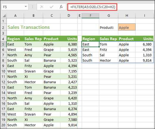
The FILTER function allows you to filter a range of data based on criteria you define.
In the following example we used the formula =FILTER(A5:D20,C5:C20=H2,»») to return all records for Apple, as selected in cell H2, and if there are no apples, return an empty string («»).
The FILTER function filters an array based on a Boolean (True/False) array.
The array, or range to filter
A Boolean array whose height or width is the same as the array
The value to return if all values in the included array are empty (filter returns nothing)
An array can be thought of as a row of values, a column of values, or a combination of rows and columns of values. In the example above, the source array for our FILTER formula is range A5:D20.
The FILTER function will return an array, which will spill if it’s the final result of a formula. This means that Excel will dynamically create the appropriate sized array range when you press ENTER. If your supporting data is in an Excel table, then the array will automatically resize as you add or remove data from your array range if you’re using structured references. For more details, see this article on spilled array behavior.
If your dataset has the potential of returning an empty value, then use the 3rd argument ( [if_empty]). Otherwise, a #CALC! error will result, as Excel does not currently support empty arrays.
If any value of the include argument is an error (#N/A, #VALUE, etc.) or cannot be converted to a Boolean, the FILTER function will return an error.
Excel has limited support for dynamic arrays between workbooks, and this scenario is only supported when both workbooks are open. If you close the source workbook, any linked dynamic array formulas will return a #REF! error when they are refreshed.
Examples
FILTER used to return multiple criteria
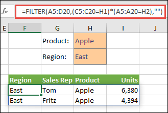
In this case, we’re using the multiplication operator (*) to return all values in our array range (A5:D20) that have Apples AND are in the East region: =FILTER(A5:D20,(C5:C20=H1)*(A5:A20=H2),»»).
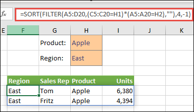
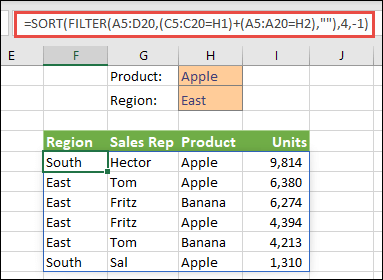
FILTER used to return multiple criteria and sort
In this case, we’re using the previous FILTER function with the SORT function to return all values in our array range (A5:D20) that have Apples AND are in the East region, and then sort Units in descending order: =SORT(FILTER(A5:D20,(C5:C20=H1)*(A5:A20=H2),»»),4,-1)
In this case, we’re using the FILTER function with the addition operator (+) to return all values in our array range (A5:D20) that have Apples OR are in the East region, and then sort Units in descending order: =SORT(FILTER(A5:D20,(C5:C20=H1)+(A5:A20=H2),»»),4,-1).
Notice that none of the functions require absolute references, since they only exist in one cell, and spill their results to neighboring cells.
Need more help?
You can always ask an expert in the Excel Tech Community or get support in the Answers community.
Источник
Filter data in a range or table
Try it!
Use filters to temporarily hide some of the data in a table, so you can focus on the data you want to see.
Filter a range of data
Select any cell within the range.
Select Data > Filter.

Select the column header arrow  .
.
Select Text Filters or Number Filters, and then select a comparison, like Between.

Enter the filter criteria and select OK.

Filter data in a table
When you Create and format tables, filter controls are automatically added to the table headers.
Select the column header arrow for the column you want to filter.
Uncheck (Select All) and select the boxes you want to show.

The column header arrow changes to a Filter icon. Select this icon to change or clear the filter.
Источник
Quick start: Filter data by using an AutoFilter
By filtering information in a worksheet, you can find values quickly. You can filter on one or more columns of data. With filtering, you can control not only what you want to see, but what you want to exclude. You can filter based on choices you make from a list, or you can create specific filters to focus on exactly the data that you want to see.
You can search for text and numbers when you filter by using the Search box in the filter interface.
When you filter data, entire rows are hidden if values in one or more columns don’t meet the filtering criteria. You can filter on numeric or text values, or filter by color for cells that have color formatting applied to their background or text.

Select the data that you want to filter
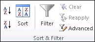
On the Data tab, in the Sort & Filter group, click Filter.
Click the arrow in the column header to display a list in which you can make filter choices.
Note Depending on the type of data in the column, Microsoft Excel displays either Number Filters or Text Filters in the list.

Filter by selecting values or searching
Selecting values from a list and searching are the quickest ways to filter. When you click the arrow in a column that has filtering enabled, all values in that column appear in a list.

1. Use the Search box to enter text or numbers on which to search
2. Select and clear the check boxes to show values that are found in the column of data
3. Use advanced criteria to find values that meet specific conditions
To select by values, in the list, clear the (Select All) check box. This removes the check marks from all the check boxes. Then, select only the values you want to see, and click OK to see the results.
To search on text in the column, enter text or numbers in the Search box. Optionally, you can use wildcard characters, such as the asterisk ( *) or the question mark ( ?). Press ENTER to see the results.

Filter data by specifying conditions
By specifying conditions, you can create custom filters that narrow down the data in the exact way that you want. You do this by building a filter. If you’ve ever queried data in a database, this will look familiar to you.
Point to either Number Filters or Text Filters in the list. A menu appears that allows you to filter on various conditions.
Choose a condition and then select or enter criteria. Click the And button to combine criteria (that is, two or more criteria that must both be met), and the Or button to require only one of multiple conditions to be met.
Click OK to apply the filter and get the results you expect.
Next steps
Experiment with filters on text and numeric data by trying the many built-in test conditions, such as Equals, Does Not Equal, Contains, Greater Than, and Less Than. For more information, see Filter data in a range or table.
Note Some of these conditions apply only to text, and others apply only to numbers.
Create a custom filter that uses multiple criteria. For more information, see Filter by using advanced criteria.
Источник
What Is Filtering In Excel?
Filtering data in MS Excel refers to displaying only the rows that meet certain conditions. (The other rows gets hidden.) Using the store data, if you are interested in seeing data where Shoe Size is 36, then you can set filter to do this.
What is the purpose of filtering data?
Filtering Data
When data is filtered, only rows that meet the filter criteria will display and other rows will be hidden. With filtered data, you can then copy, format, print, etc., your data, without having to sort or move it first.
What is Sorting and filtering Excel?
The filter tool gives you the ability to filter a column of data within a table to isolate the key components you need.The sorting tool allows you to sort by date, number, alphabetic order and more.
Why is filtering important in Excel?
Filtering data in a spreadsheet allows only certain data to display. This function is useful when you want to focus on specific information in a large dataset or table.
What do you mean by filtering?
1 : to subject to the action of a filter. 2 : to remove by means of a filter. intransitive verb. 1 : to pass or move through or as if through a filter. 2 : to come or go in small units over a period of time people began filtering in.
What is difference between filtering and sorting?
Essentially, sorting and filtering are tools that let you organize your data. When you sort data, you are putting it in order. Filtering data lets you hide unimportant data and focus only on the data you’re interested in.
What is the difference between short and filter?
Sorting means to arrange the give data according to a particular field, either in ascending order or in descending order. The filter feature selectively blocks out data you don’t want to see.
What is custom filtering?
Custom filter is a module that allows you to create your own filters based on regular expressions.
When would you want to filter data in Excel?
By filtering information in a worksheet, you can find values quickly. You can filter on one or more columns of data. With filtering, you can control not only what you want to see, but what you want to exclude.
What is filter give example?
The definition of a filter is something that separates solids from liquids, or eliminates impurities, or allows only certain things to pass through. A Brita that you attach to your water faucet to remove impurities from your water is an example of a water filter.
What do you mean by filtering in computer?
1) In computer programming, a filter is a program or section of code that is designed to examine each input or output request for certain qualifying criteria and then process or forward it accordingly. This term was used in UNIX systems and is now used in other operating systems.
What is filtering data in computer?
Data filtering is the task of reducing the content of noise or errors from measured process data. It is an important task because measurement noise masks the important features in the data and limits their usefulness in practice.
What is filter in computer class 10?
Filtering is a useful way to see only the data that you want displayed. You can use filters to display specific records in a form, report, query, or datasheet, or to print only certain records from a report, table, or query.
What do you mean by filtering data Class 10?
Filtering is a process where we can see only data as per defined criteria. Suppose a table has data of sales figure of 10 products for 5 years. We can select a filter for one particular product & see its data only. We can apply multiple filters.
What is the difference between sieving from filtering?
In sieving, particles that are too big to pass through the holes of the sieve are retained (see particle size distribution). In filtration, a multilayer lattice retains those particles that are unable to follow the tortuous channels of the filter.
What are the advantages of sorting and filtering data?
Benefits of sorting and filtering data –
- Systematic representation – sorting enables users to represent the data in a very systematic manner that enables fine presentation.
- Better understanding of data – when data is presented in a sorted and filtered manner then then data decoding and understanding becomes very easy.
How do I copy filtered data in Excel?
Follow these steps:
- Select the cells that you want to copy For more information, see Select cells, ranges, rows, or columns on a worksheet.
- Click Home > Find & Select, and pick Go To Special.
- Click Visible cells only > OK.
- Click Copy (or press Ctrl+C).
What is the difference between filtering data by selection and filtering data by form?
Filter by Selection: To filter all the rows in a table that contain a value that matches a selected value in a row by filtering the datasheet view. Filter by form: To filter on several fields in a form or datasheet, or if you are trying to find a specific record.
What are steps to filter data in a table?
Try it!
- Select any cell within the range.
- Select Data > Filter.
- Select the column header arrow .
- Select Text Filters or Number Filters, and then select a comparison, like Between.
- Enter the filter criteria and select OK.
What is Result Filter in MVC?
Result filters are executed before or after generating the result for an action. The Action Result type can be ViewResult, PartialViewResult, RedirectToRouteResult, which derives from the ActionResult class. Example: public interface IResultFilter.
What is custom filtering give one example?
One of the most common uses of a Custom Filter is screening transactions for fraudulent use of credit card account numbers.Use Custom Filters and the Product Watch List to hold certain products (such as computers or televisions) when a large number are found in a single order.
Источник
The FILTER function «filters» a range of data based on supplied criteria. The result is an array of matching values from the original range. In plain language, the FILTER function will extract matching records from a set of data by applying one or more logical tests. Logical tests are supplied as the include argument and can include many kinds of formula criteria. For example, FILTER can match data in a certain year or month, data that contains specific text, or values greater than a certain threshold.
The FILTER function takes three arguments: array, include, and if_empty. Array is the range or array to filter. The include argument should consist of one or more logical tests. These tests should return TRUE or FALSE based on the evaluation of values from array. The last argument, if_empty, is the result to return when FILTER finds no matching values. Typically this is a message like «No records found», but other values can be returned as well. Supply an empty string («») to display nothing.
The results from FILTER are dynamic. When values in the source data change, or the source data array is resized, the results from FILTER will update automatically. Results from FILTER will «spill» onto the worksheet into multiple cells.
Basic example
To extract values in A1:A10 that are greater than 100:
=FILTER(A1:A10,A1:A10>100)
To extract rows in A1:C5 where the value in A1:A5 is greater than 100:
=FILTER(A1:C5,A1:A5>100)
Notice the only difference in the above formulas is that the second formula provides a multi-column range for array. The logical test used for the include argument is the same.
Note: FILTER will return a #CALC! error if no matching data is found
Filter for Red group

In the example shown above, the formula in F5 is:
=FILTER(B5:D14,D5:D14=H2,"No results")
Since the value in H2 is «red», the FILTER function extracts data from array where the Group column contains «red». All matching records are returned to the worksheet starting from cell F5, where the formula exists.
Values can be hardcoded as well. The formula below has the same result as above with «red» hardcoded into the criteria:
=FILTER(B5:D14,D5:D14="red","No results")
No matching data
The value for is_empty is returned when FILTER does not find matching results. If a value for if_empty is not provided, FILTER will return a #CALC! error if no matching data is found:
=FILTER(range,logic) // #CALC! error
Often, is_empty is configured to provide a text message to the user:
=FILTER(range,logic,"No results") // display message
To display nothing when no matching data is found, supply an empty string («») for if_empty:
=FILTER(range,logic,"") // display nothing
Values that contain text
To extract data based on a logical test for values that contain specific text, you can use a formula like this:
=FILTER(rng1,ISNUMBER(SEARCH("txt",rng2)))
In this formula, the SEARCH function is used to look for «txt» in rng2, which would typically be a column in rng1. The ISNUMBER function is used to convert the result from SEARCH into TRUE or FALSE. Read a full explanation here.
Filter by date
FILTER can be used with dates by constructing logical tests appropriate for Excel dates. For example, to extract records from rng1 where the date in rng2 is in July you can use a generic formula like this:
=FILTER(rng1,MONTH(rng2)=7,"No data")
This formula relies on the MONTH function to compare the month of dates in rng2 to 7. See full explanation here.
Multiple criteria
At first glance, it’s not obvious how to apply multiple criteria with the FILTER function. Unlike older functions like COUNTIFS and SUMIFS, which provide multiple arguments for entering multiple conditions, the FILTER function only provides a single argument, include, to target data. The trick is to create logical expressions that use Boolean algebra to target the data of interest and supply these expressions as the include argument. For example, to extract only data where one value is «A» and another is greater than 80, you can use a formula like this:
=FILTER(range,(range="A")*(range>80),"No data")
The math operation of addition (*) joins the two conditions with AND logic: both conditions must be TRUE in order for FILTER to retrieve the data. See a detailed explanation here.
Complex criteria
To filter and extract data based on multiple complex criteria, you can use the FILTER function with a chain of expressions that use boolean logic. For example, the generic formula below filters based on three separate conditions: account begins with «x» AND region is «east», and month is NOT April.
=FILTER(data,(LEFT(account)="x")*(region="east")*NOT(MONTH(date)=4))
See this page for a full explanation. Building criteria with logical expressions is an elegant and flexible approach that can be extended to handle many complex scenarios. See below for more examples.
Notes
- FILTER can work with both vertical and horizontal arrays.
- The include argument must have dimensions compatible with the array argument, otherwise FILTER will return #VALUE!
- If the include array includes any errors, FILTER will return an error.
The Excel Filter Feature is a great tool that proves to be a lifesaver at the time when you are working with huge data in Excel. In this blog, we would unlock this filter feature in Excel. We would learn how to filter huge data in excel. We would also get into answering the following common questions – how to filter values, or numbers, or dates and time in Excel, how to use filter using wildcard characters in excel, how to filter using the search box, how to filter by text or cell color.
Sample Data – Download Sample File
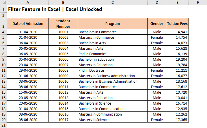
In this blog, we would be using the below data. Kindly download and practice along with using the Download button.
Table of Contents
- Sample Data – Download Sample File
- What is the Purpose of Filter Feature in Excel?
- Adding Filter Option on Header Rows
- Simple Ways to Filter Your Data Set in Excel
- Applying Filter on Single Column
- Applying Filter on Multiple Columns
- Filter Data Using Filter Search Box in Excel
- Clearing Filter on Columns in Excel
- How to Filter Values or Text in Excel?
- Filter Values based on Two Criteria
- How to Filter Numbers in Excel?
- How to Filter Dates in Excel?
- How to Filter By Color in Excel?
- Quick Way to Filter By A Specific Cell’s Value, Font Color, Cell Color or Icon
- A Solution To – AutoFilter Does Not Work After Changing Data
- Copy and Paste only Filtered Data in Excel
- Copy and Paste Filtered Data Including Header Row
- Copy and Paste Filtered Data Excluding Header Row
- Removing Filter From Headers in Excel
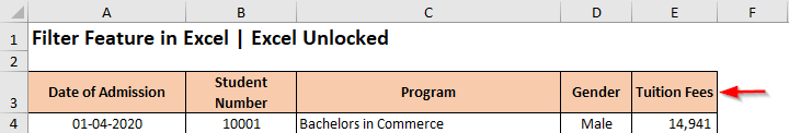
What is the Purpose of Filter Feature in Excel?
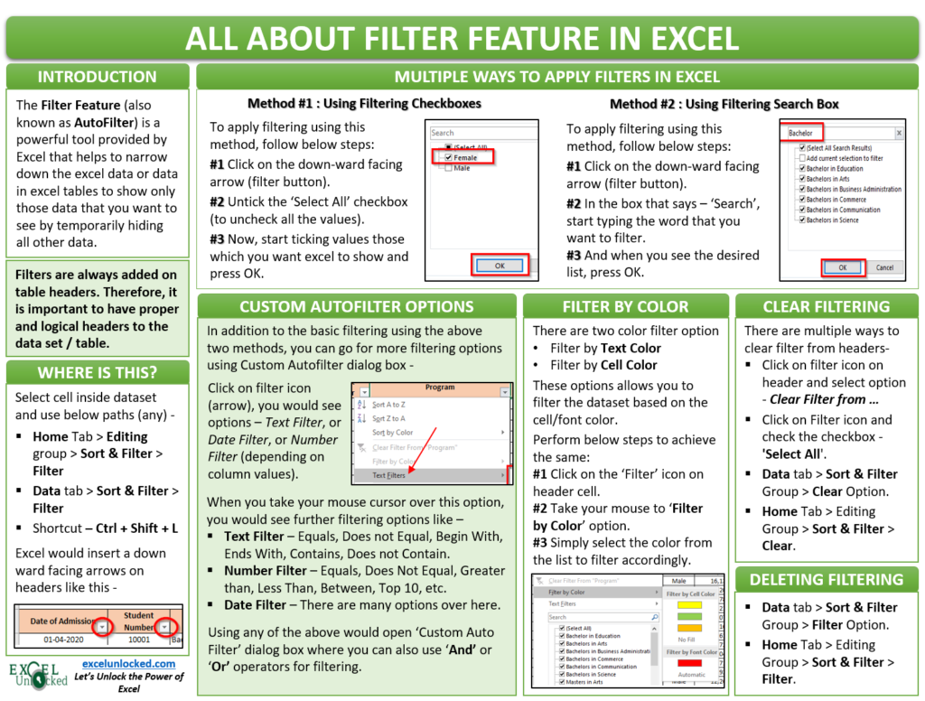
The Filter Feature (also known as AutoFilter) is a powerful tool provided by Excel that narrows down the excel data or data in excel tables to show only those data that you want to see by temporarily hiding all other data. In our sample data, for example, we can use this feature to condense the data such that it only shows the programs taken up by the ‘Female‘ applicants.
In a similar way, you can filter by dates, or values or by any other such criteria.
The filters are always added to the headers of the data set. Therefore, it is important that your excel data must contain a header row, with logical headings. In our example, row 3 is the header row with headings describing the column data.
Once your dataset has proper headers, you are now good to insert the AutoFilter on these headers. To add AutoFilter on the header row, click on any of the cells inside the excel data set (like C7) and use any of the below-mentioned ways:
- Go to ‘Home‘ tab > ‘Editing‘ Group > ‘Sort & Filter‘ Option > ‘Filter‘ button.
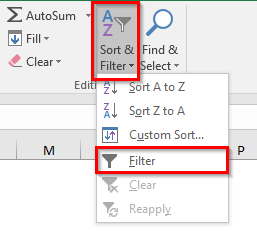
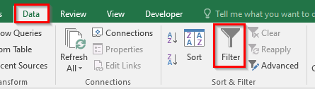
- Go to ‘Data‘ tab > ‘Sort & Filter‘ group > ‘Filter‘ Button.
- Keyboard Shortcut Method : Ctrl + Shift + L
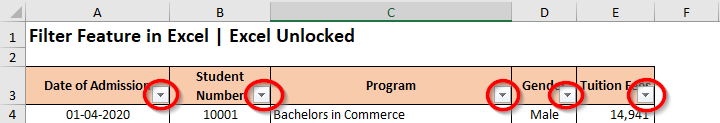
As soon as you use any of the above methods, the excel would automatically detect the header row inside the table or data set and insert filter buttons on each of the header cells. These are the downward-facing arrows, like the way shown below:
Simple Ways to Filter Your Data Set in Excel
Once the filter option added to the headers, you are good to start filtering your data set.
With this feature, you can filter your data by a single column or by multiple columns.
Applying Filter on Single Column
To apply the filter on a single column, simply click on the filter button (downward-facing arrow) of the respective column. (Let us firstly apply the filter on the column ‘Program Name’). As a result, you would notice that all the checkboxes are checked by default.
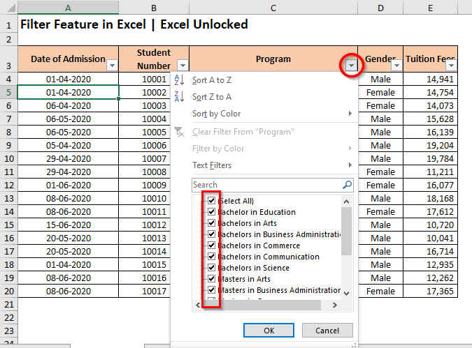
Uncheck the checkbox that says ‘Select All‘. This would remove the check boxes from all the values.
Now, start ticking the values that you wish to view and click on ‘OK’, like the way demonstrated in the below image.
Consequently, the excel would view or show only the selected values in the column, rest all are hidden. Don’t worry excel has not deleted them, they are still there in the backend.
Applying Filter on Multiple Columns
In a similar way, you can apply the filter on other columns in the Excel Data Table. There is no limitation on how many columns to which you can apply the filter.
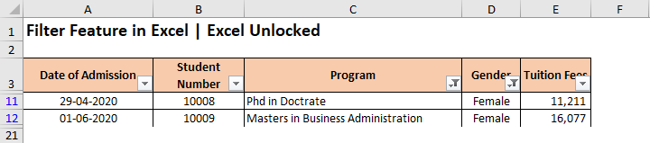
Let us now apply another filter on the column having header – ‘Gender‘.
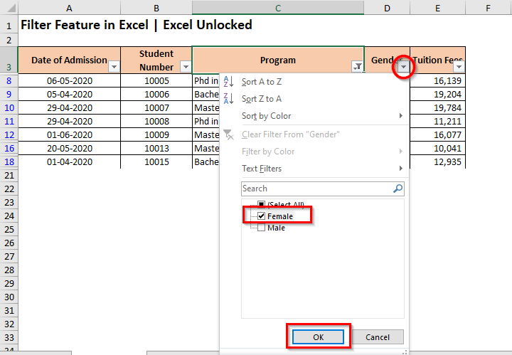
As a result, the excel would now only display the data set rows for selected ‘Program’ and for ‘Female’ candidates. All others are temporarily hidden (not removed).
Some Useful Points and Tips
Once a filter is applied on the header row-
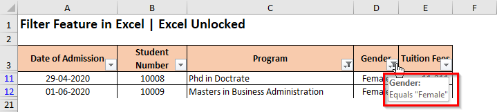
- The Downward-facing arrow on the filtered column changes its icon which denotes that there is a filter applied to this column.
- When you take your mouse cursor over the filter button, it shows the filter values.
- To increase or decrease the width of the filter window, take your mouse cursor on the bottom-right corner of the filter window. Once the mouse cursor changes to a two-side facing arrow, click and drag right (to increase) or left (to decrease). See the below demonstration for more clarity.
Filter Data Using Filter Search Box in Excel
In the earlier section, we learned about how to filter your data set by selecting the checkboxes in the Filter window. There is yet another way to filter out a specific text or value or numbers or dates/time in Excel which is by using the ‘Filter’ search box. The Filter search box is placed just above the list of values in the Filter window.
To filter your data set using the ‘Filter’ search box, simply click on the ‘Filter’ drop-down icon on the header and type the search value in the search box. As a result, the excel would narrow down the list to show only the specified values. Finally, click on the ‘OK’ button to apply the filter.
To illustrate with an example, let us filter out the ‘Program’ column with the Bachelor’s degree.
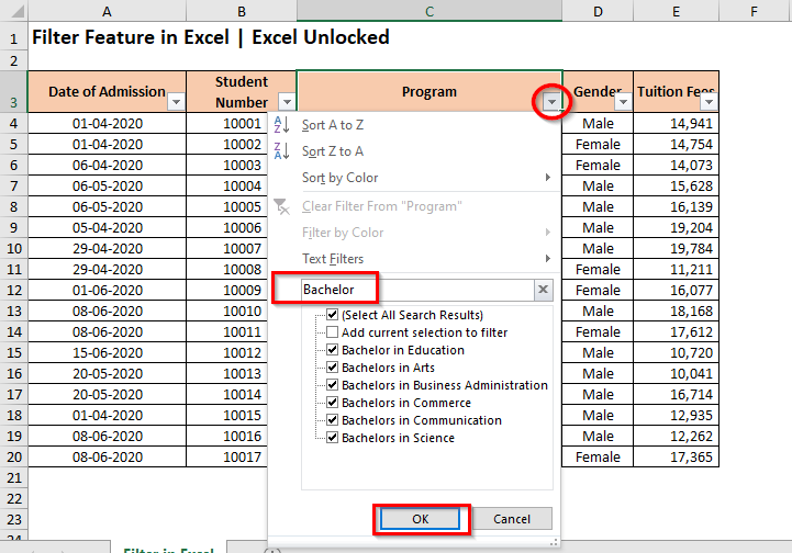
Not sure about the exact text to search, then use wildcard characters in the search box for a non-exact filter search in Excel. If you are unaware of what are wildcard characters in Excel and its usage, then please click here.
Clearing Filter on Columns in Excel
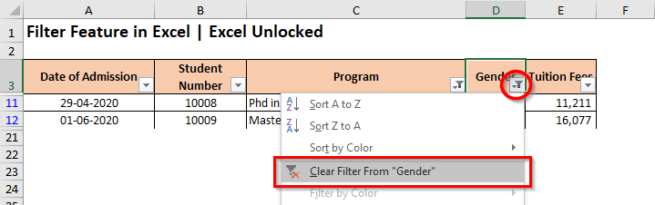
When you want to clear filter from selected or all the header columns in Excel, you can use any of the below-mentioned ways:
- Click on the ‘Filter‘ icon on the header of the column header, and click on the option that says – Clear Filter from <Column Header Name>
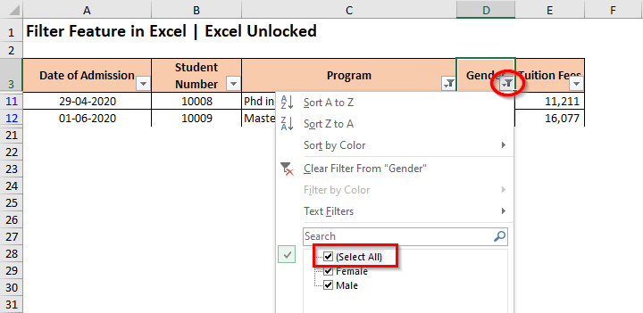
- Another way is to click on the ‘Filter‘ icon of the header, and check the checkbox – ‘Select All‘.
When you clear the filter from the column ‘Gender’, the data set would now only have a filter on the column header ‘Program’. It has only cleared filter from the row ‘Gender’ and has not touched any other filters.
To clear multiple filter from all the headers cells, use any of the following way:
- Click on any of the cells in the dataset and navigate to the path – Data tab > Sort & Filter Group and there click on the option that says – Clear.
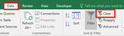
- Or you can even use this – Home Tab > Editing Group. Click the option Sort & Filter > Clear.
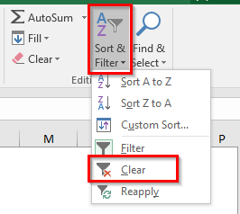
It is important to note that the above method only clears the filter from the header cell. It does not remove the filter icon from the header row. To learn how to remove the filter in Excel, wait until the end of this blog.
How to Filter Values or Text in Excel?
When you are working with text filters, there are many other text filter options available in addition to what we learned above. Below is the list of the same.
- You can filter the values or text which exactly Equals or which Does Not Equal to some text.
- Additionally, you can even filter for a non-exact match by using the Contains and Does Not Contain a text
- Or, you can even filter the values or text that starts or Begins With or Ends With a particular text.
These advanced filter options are available under the ‘Text Filter’ section of the Filter Window as shown in the image below:
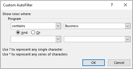
Let us understand this with the help of a small example: Let us, for example, get the program that contains the word ‘Business’ in it. To achieve it,
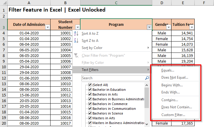
Click on the ‘Filter‘ icon on the column header – ‘Program’, and take your mouse cursor to the option – Text Filters.
In the list of options that come up, select the option that says – ‘Contains‘. As a result, the ‘Custom AutoFilter‘ dialog box would appear on your screen. In the input box besides the word ‘Contains’, write the text that you want to filter (in our case ‘Business’) and press OK.
As soon as you press OK, excel would show all the values or text that contains the word ‘Business’ and will hide all other data rows.
Note that, just like Filter search box, this ‘Custom AutoFilter’ dialog box also accepts wildcard character search.
Filter Values based on Two Criteria
The Custom AutoFilter dialog box also allows us to filter out the data rows based on two criteria. Use the And and Or operator radio buttons based on how you wish to filter.
For example: Let us filter out all the programs for Commerce and Science. In this case, as we want both the values, we shall use Or operator, like this-
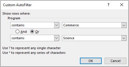
This would filter out those values which either contain the word ‘Commerce‘ or contain the word ‘Science‘.
How to Filter Numbers in Excel?
Similar to the text filter learned above, there are many additional filter options available carry Number Filters in Excel. Below is the list of the same:
- You can filter the exact number or amount by using Equals and Does Not Equal option under the ‘Number Filter’.
- Similarly, the Number Filter – Greater Than and Less Than allows us to get all values that are more or less than a specific value.
- Greater Than or Equal To and Less Than or Equal To works in a similar way.
- Between Number Filter allows you to filter out the values lies between two values (lower and upper values both inclusive)
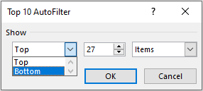
- Other options are – Top 10, Above Average, Below Average
The filter option Top 10 does not exactly only mean Top 10 values. You can change it to any other value like Top 15, or Top 27 Values, and even Bottom 5 values and so on.
How to Filter Dates in Excel?
Unlike the Text and Number Filter, the Dates Filters option allows us with more advanced filtering options. The below image in itself is self-explanatory.
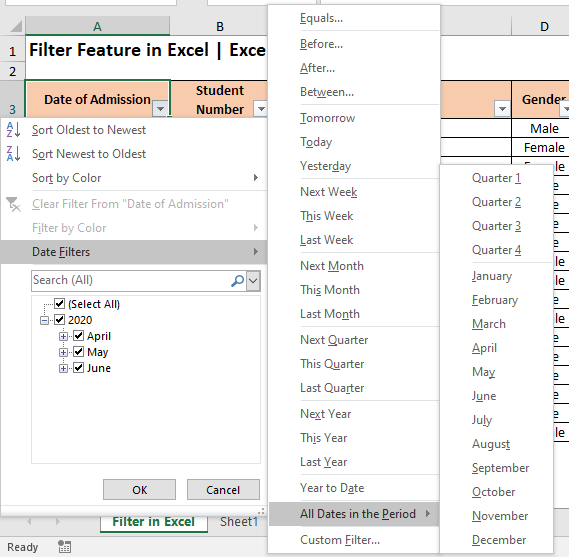
In a nutshell, below options are available for filtering dates in Excel –
- You can filter the dates which fall in the current month/week/quarter/year and even for previous and upcoming (i.e. next) month/week/quarter/year.
- Additionally, you can filter out by an exact date, or date that falls before or after a particular date, or between two dates.
- Excel provides with an option to filter all the dates in a particular month or quarter (regardless of the year in which it falls)
- You can create a custom date filter using the ‘Custom AutoFilter’ dialog box to which you are already aware of using.
Important to notice – Excel by default groups all the dates by year, months, and then the days. You can expand or collapse the groups (year, months, and days) to filter the dates and check/uncheck it to filter accordingly.
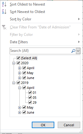
In the above image, you can see that all the dates are grouped by years first (2020 and 2019). Within the years there are months and then the days in the month. If you clear the checkbox for 2020, then the excel would only show the dates that lie in 2019.
How to Filter By Color in Excel?
When the data set contains any text with color or any cell with a background color, you can use the ‘Filter by Color‘ option in the ‘Filter’ Window to filter the dataset by a specific text or cell background color.
Let me explain this with a small example. I am changing the background color of different cells to yellow, orange, and green. Also, I have the font color in a few of the cells as ‘Red’.
To filter the values based on color, simply click on the ‘Filter’ drop-down arrow button on the header cell and take your mouse cursor over the option that says – ‘Filter by Color’.
As a result, you would see that excel lists all the cell and font color. You can choose the color that you want to filter with.

Let us, for example, filter the programs by Red font color. The result of the filter would be as below.
Quick Way to Filter By A Specific Cell’s Value, Font Color, Cell Color or Icon
Instead of using the ‘Filter’ drop-down icon to filter, you can even filter the dataset based on a specific cell’s value, icon, or font and cell color. To do so, follow the undermentioned steps:
- Right-click on the cell that contains the color by which you want to filter. Let us, in this case, filter by yellow color. Therefore, I have right-clicked on C4 (as it has a yellow cell color).
- Take your mouse cursor to the option that says – ‘Filter‘, and click on the option – ‘Filter by Selected Cell’s Color‘.
As a result, excel would filter the dataset based on the cell color – Yellow, as demonstrated in the below image:
A Solution To – AutoFilter Does Not Work After Changing Data
When you make any changes in the filtered data, you would notice that excel does not refresh the filter automatically. Yes, that is absolutely true. You need to reapply the filter in order to refresh the data and apply the filter on the changed data. There are a couple of ways to do the same, as listed below:
- Using Filter Window – After making changes in the filtered data, simply click on the ‘Filter’ drop-down arrow on the header cell and click ‘OK’ in there. However, there is are exceptions to this method. This would not work when you apply ‘filter by color’ or ‘Number Filter/Text Filter/Date Filter’. This technique only applies when you use the search box to filter out the data.
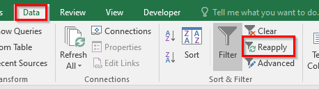
- Using Reapply Option – After making changes in the filtered data, simply navigate to the Data tab > Sort & Filter Group > Reapply Option. The keyboard shortcut key for the same is Ctrl + Alt + L.
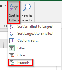
This option is also available in the Home Tab > Editing Group > Sort & Filter Option > Reapply.
Copy and Paste only Filtered Data in Excel
There are two possibilities to copy and paste only filtered data in Excel.
Copy and Paste Filtered Data Including Header Row
Simply, click on any of the cell in the filtered area, and press Ctrl + A to select the entire excel table or data set. As a result, you would notice that excel selects the entire table including both data rows as well as the header row. Now, press Ctrl + C to copy the selection and use Ctrl + V at the destination location to paste the filtered data cells.
Copy and Paste Filtered Data Excluding Header Row
To copy and paste only filtered data (without header row), select the top-left cell of the data (which in our case it is C4). Press keyboard keys Ctrl + Shift + Down_Arrow and then press Ctrl + Shift + Right_Arrow (instead you can even use Ctrl + Shift + End). Any of these ways would select the entire data set (excluding headers). Now, use Ctrl + C to copy the selection and then Ctrl + V to paste the filtered data set at the destination cell.
Usually, when you copy the filtered dataset using the above methods, excel does not include the hidden rows in the copy area. The hidden rows are excluded and it only takes the visible rows while copying. However, sometimes when your data is huge, it may not work in expected behavior. In those cases, to play safe, you can use the GoTo (F5) > Special > Visible Cells Only feature to select only the visible rows. The keyboard shortcut for the same is Alt + ; (semi-colon).
Finally, let us now learn how to remove filters from the excel header row. There are multiple ways using which you can remove filters, as listed below-
- The easiest way is to use the keyboard shortcut – Ctrl + Shift + L.
- Another way is to use ribbon path – Data Tab > Sort & Filter Group > Filter option OR Home Tab > Editing Group > Sort & Filter Option > Filter Option.
RELATED POSTS
-
How to Make A Table In Excel – A Hidden Functionality
-
How to Sort a Table or Data in Excel
-
Text and Number Filter in Pivot Table in Excel
-
Group and Ungroup Rows in Excel
-
FILTER Function in Excel – Dynamic Filtered Range
-
Applications – FILTER Function in Excel
There are many built-in Excel tools to help with data management and the sorting and filtering features are among the best. The filter tool gives you the ability to filter a column of data within a table to isolate the key components you need. The sorting tool allows you to sort by date, number, alphabetic order and more. In the following example, we will explore the usage of sorting and filtering and show some advanced sorting techniques.
For today’s example, we will use the following spreadsheet:

As you can see, the order dates, order numbers, prices, etc. are all out of order. Let’s get started on running some sorting and filtering techniques.
Sorting Data
Let’s say you had the spreadsheet above and wanted to sort by price. This process is fairly simple. You can either highlight the whole column or even click on the first cell in the column to get started. Then you will:
- Right click to open the menu
- Go down to the Sort option – when hovering over Sort the sub-menu will appear
- Click on Largest to Smallest
- Select Expand the selection
- Click OK
The whole table has now adjusted for the sorted column. Note: when the data in one column is related to the data in the remaining columns of the table, you want to select Expand the selection. This will ensure the data in that row carries over with sorted column data.
Filtering Data
The filter feature applies a drop down menu to each column heading, allowing you to select specific choices to narrow a table. Using the above example, let’s say you wanted to filter your table by Company and Salesperson. Specifically, you want to find the number of sales Dylan Rogers made to Eastern Company.
To do this using the filter you would:
- Go to the Data tab on Excel ribbon
- Select the Filter tool
- Select Eastern Company from the dropdown menu
- Select Dylan Rogers from the Salesperson dropdown menu
Boom – you now have the exact number of sales Dylan Rogers made to Eastern Company.
The Sort & Filter Tool
In addition to the right-click menu sorting option and the Filter tool on the Data ribbon, Excel has a Sort & Filter tool that allows for custom sorting.
In the following GIF, we can see how the Custom Sorting tool can be used to sort date ranges or price ranges.
But notice how this example is either/or. What if you wanted to sort by date and by price? This where the Custom Sort option really comes in handy. After selecting your first sorting conditions, you can add a level to get event more accurate data:
As you can see, Excel offers a variety of sorting and filtering tools to help you refine your data and keep it organized. We hope you found today’s tips useful. Now go out there and get your data sorted!
Use Learn Excel Now to help with all your Excel questions and training needs. We’re not just experts in Excel, there is content, free resources, and training courses available for Word, Outlook and more.
Download our free templates and guides
Receive live webinars from industry experts
Train at your own pace with our on-demand training

The FILTER function in Excel is a very useful and frequently used function, that you will likely find the need for in many situations. Note that the FILTER function is only available in Microsoft Office 365, and Microsoft Office Online.
To filter by using the FILTER function in Excel, follow these steps:
- Type =FILTER( to begin your filter formula
- Type the address for the range of cells that contains the data that you want to filter, such as B1:C50
- Type a comma, and then type the condition for the filter, such as C3:C50>3 (To set a condition, first type the address of the «criteria column» such as B1:B, then type an operator symbol such as greater than (>), and then type the criteria, such as the number 3.
- Type a closing parenthesis and then press enter on the keyboard. Your entire formula will look like this: =FILTER(B1:C50,C1:C50>3)
In this article I will start with the basics of using the FILTER function (examples included), and then also show you some more involved ways of using the FILTER function. This article focuses specifically on the FILTER function that is typed into the spreadsheet cells as a formula, and not the filter command available from the toolbar and pop-up menus.
Using the FILTER function in Excel is almost the same as using it in Google Sheets, but there are slight differences between the two. Click here to read the Google Sheets version of this article
Here are the Excel Filters formulas:
Filter by a number
- =FILTER(A3:B12, B3:B12>0.7)
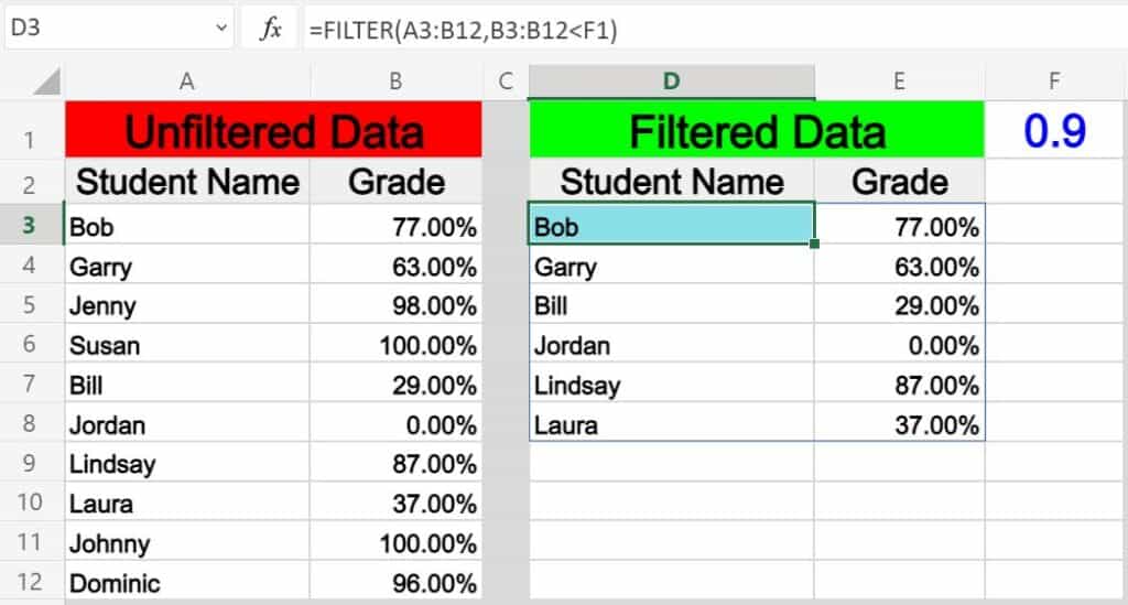
Filter by a cell value
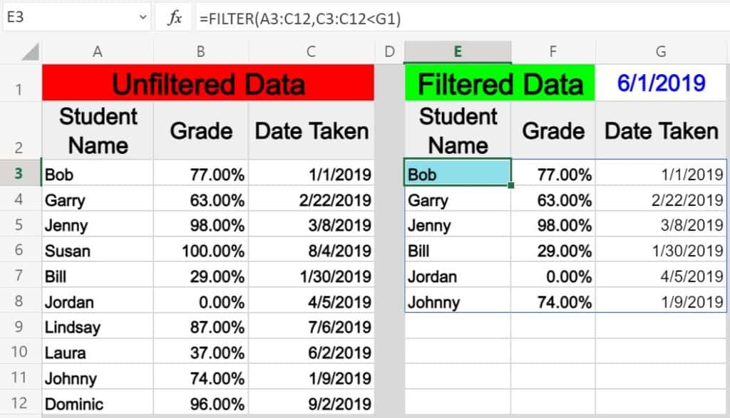
- =FILTER(A3:B12, B3:B12<F1)
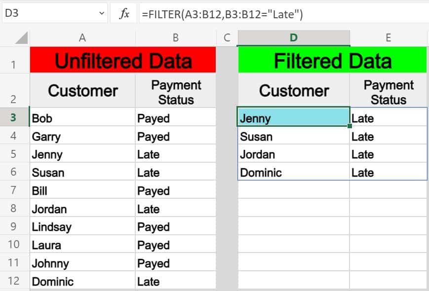
Filter by a text string
- =FILTER(A3:B12, B3:B12=»Late»)
Filter where NOT equal to
- =FILTER(A3:E1000, B3:B1000<>»Bob»)
Filter by date
- =FILTER(A3:C12,C3:C12<G1) (Date entered in cell G1)
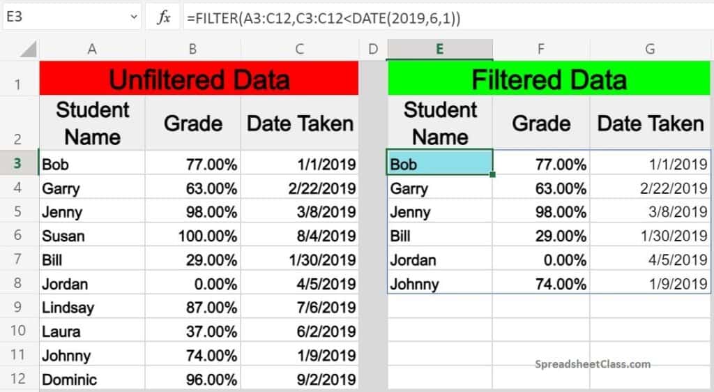
- =FILTER(A3:C12,C3:C12<DATE(2019,6,1))
Filter by multiple conditions
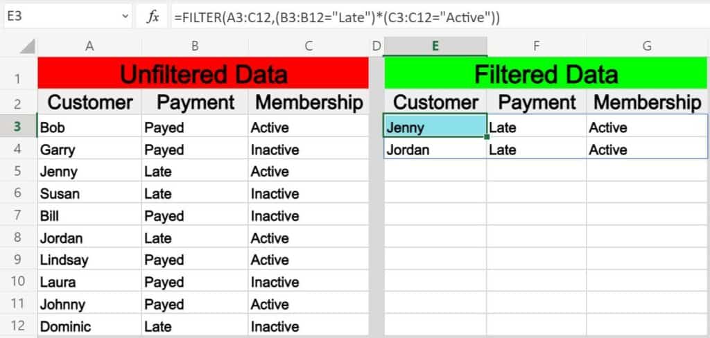
- =FILTER(A3:C12,(B3:B12=»Late»)*(C3:C12=»Active»)) (AND logic)
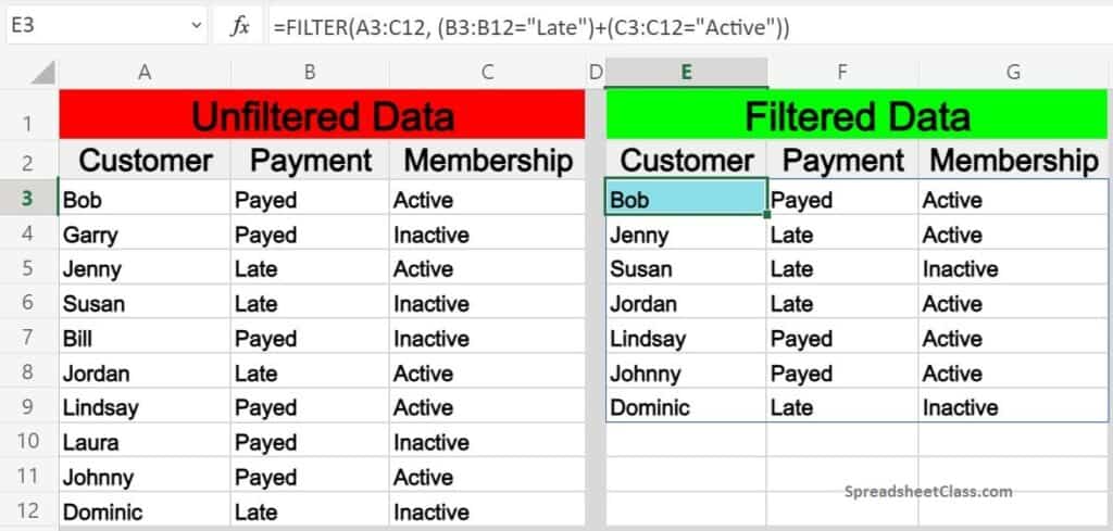
- =FILTER(A3:C12, (B3:B12=»Late»)+(C3:C12=»Active»)) (OR logic)
Filter from another sheet
- =FILTER(‘Sheet Name’!A3:B12,’Sheet Name’!B3:B12=»Full Time»)
=FILTER(A3:B12, B3:B12=F1)
(Copy/Paste the formula above into your sheet and modify as needed)
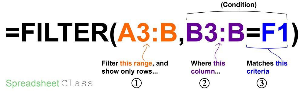
The FILTER function in Excel allows you to filter a range of data by a specified condition, so that a new set of data will be displayed which only shows the rows/columns from the original data set that meets the criteria/condition set in the formula.
Excel description for FILTER function:
Syntax:
=FILTER(array,include,[if_empty])Formula summary: “The FILTER function filters an array based on a Boolean (True/False) array.”
array (Required): The array, or range to filter
include (Required): A Boolean array whose height or width is the same as the array
[if_empty] (Optional): The value to return if all values in the included array are empty (filter returns nothing)
The source range that you want to filter, can be a single column or multiple columns.
The range that is used to check against the criteria that you set, must be a single column (later I will show you how to filter by multiple conditions, but don’t worry about that for now).
The criteria that set in the condition can be manually typed into the formula as a number or text, or it can also be a cell reference.
*Note that the source range and the single column range for the condition, must be the same size (must contain the same number of rows), or the cell will display an error.
Filtering by a single condition in Excel
First let’s go over using the FILTER function in Excel in its simplest form, with a single condition/criteria.
I will show you how to filter by a number, a cell value, a text string, a date… and I will also show you how to use varying «operators» (Less than, Equal to, etc…) in the filter condition.
Part 1: How to filter by a number
In this first example on how to use the filter function in Excel, the scenario is that we have a list of students and their grades, and that we want to make a filtered list of only students who have a perfect grade.
The task: Show a list of students and their scores, but only those that have a perfect grade
The logic: Filter the range A3:B12, where the column B3:B12 is greater than 0.7 (70%)
The formula: The formula below, is entered in the blue cell (D3), for this example
=FILTER(A3:B12, B3:B12>0.7)
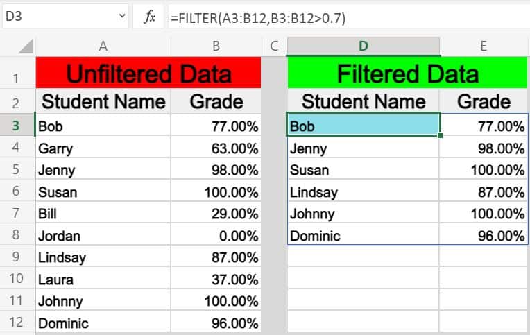
Operators that can be used in the FILTER function:
In this example we are using the operator «=» (Equal To) for the filter condition/criteria, but you can also use any of the following:
«=» (Equals)
«>» (Greater than)
«<» (Less than)
«<>» (Not equal to)
«>=» (Greater than or equal to)
«<=» (Less than or equal to)
Part 2: How to filter by a cell value in Excel
In this example, we want to achieve the same goal as discussed above, but rather than typing the condition that we want to filter by directly into the formula, we are using a cell reference.
When you filter by a cell value in Excel, your sheet will be setup so that you can change the value in the cell at any time, which will automatically update the value that the filter criteria it attached to.
In this example, you will notice that instead of directly typing the number “0.9” into the formula itself, the filter criteria is set as cell G1, where the “0.9” value is entered.
The task: Show a list of students and their scores, but only those that have a score below 90%
The logic: Filter the range A3:B12, where B3:B12 is less than the value that is entered in the cell F1 (0.9)
The formula: The formula below, is entered in the blue cell (D3), for this example
=FILTER(A3:B12, B3:B12<F1)
Part 3: How to filter by text in Excel
In this example, we are going to use a text string as the criteria for the filter formula. This is very similar to using a number, except that you must put the text that you want to filter by inside of quotation marks.
In this scenario we are filtering a list that shows customers and their payment status, and we want to display only customers that have a payment status of “Late”.
The task: Show a list of customers who are past due on their payments
The logic: Filter the range A3:B12, where B3:B12 equals the text, “Late”
The formula: The formula below, is entered in the blue cell (D3), for this example
=FILTER(A3:B12, B3:B12=»Late»)
Part 4: Using NOT EQUAL TO in the Excel FILTER function
Now that you have got a basic understanding of how to use the filter function in Excel, here is another example of filtering by a string of text, but in this example we will use the «not equal» operator (<>), so that you can learn how to filter a range and output data that is NOT equal to criteria that you specify.
In this example we will also use a larger data set to demonstrate a more extensive application of the FILTER function in the real world.
You may be surprised at how often a situation comes up when you need to filter data where it is “not equal to” a certain number or piece of text that you specify.
In this example let’s say that we have a report/spreadsheet that shows data from sales calls that occur at your company, and we want to filter the data so that a specified sales rep (Bob) is NOT included in the filter output.
The task: Show sales call data for all sales reps, except Bob
The logic: Filter the range A2:E1000, where B2:B1000 DOES NOT equal the text, “Bob”
The formula: The formula below, is entered in the blue cell (G3), for this example
=FILTER(A3:E1000, B3:B1000<>»Bob»)
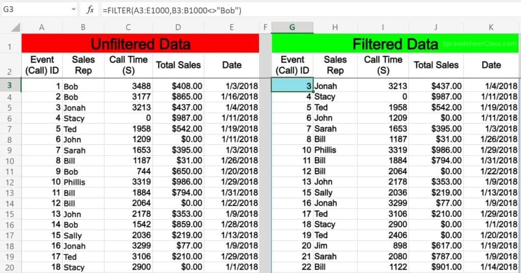
Notice that the filtered data on the right side of the image above does not contain any of the rows/calls that Bob was involved in.
Part 4: How to filter by date in Excel
Filtering by a date in Excel can be done in a couple of ways, which I will show you below. If you try to type a date into the FILTER function like you normally would type into a cell… the formula will not work correctly.
So you can either type the date that you want to filter by into a cell, and then use that cell as a reference in your formula… or you can use the DATE function.
When filtering by date you can use the same operators (>, <, =, etc…) as in other FILTER function applications. In Excel each different day/date is simply a number that is put into a special visual format. For example, in Excel, the date «06/01/2019» is simply the number «43,617», but displayed in date format. When you add one day to the date, this number increments by one each time… i.e «43,618» «43,619» «43,620»
So, one date can be considered to be «greater than» another date, if it is further in the future. Conversely, one date can be said to be «less than» another date, if it is further in the past.
In this first example we will filter by a date by using a cell reference. This is similar to the example we went over in part 2, but in this example instead of working with percentages, we are dealing with dates.
Let’s say that we want to filter a list of students, their test scores, and the dates that the tests were completed… and we want to show only tests that were taken before June (06/01/2019).
Filter by date in Excel example 1:
The task: Show only tests that were taken before June
The logic: Filter the range A3:C12, where C3:C12 is less than the date that is entered in cell G1 (06/01/2019)
The formula: The formula below, is entered in the blue cell (E3), for this example
=FILTER(A3:C12,C3:C12<G1)
Filter by date in Excel example 2:
In this second example on filtering by date in Excel we are using the same data as above, and trying to achieve the same results… but instead of using a cell reference, we will use the DATE function so that you can type enter the date directly into the FILTER function.
When using the DATE function to designate a certain date, you must first enter the year, then the month, and then the day… each separated by commas (shown below).
The task: Show only tests that were taken before June
The logic: Filter the range A3:C12, where C3:C12 is less than the date of (06/01/2019)
The formula: The formula below, is entered in the blue cell (E3), for this example
=FILTER(A3:C12,C3:C12<DATE(2019,6,1))
Filter by multiple conditions in Excel
When using the Excel FILTER function you may want to output a set of data that meets more than just one criteria. I will show you two ways to filter by multiple conditions in Excel, depending on the situation that you are in, and depending on how you want to formula to operate.
The normal way of adding another condition to your filter function, (as shown by the formula syntax in Excel), will allow you to set a second condition, where the first AND second condition must be met to be returned in filter output.
However I will also show you how to make a slight modification to the function so that you can choose to set a second condition where EITHER condition can be met to return/display in the filter function’s output/destination. (Separate the conditions with an asterisk to use AND logic, or separate the conditions with a plus sign to use AND logic.)
Part 5: Filtering by 2 conditions where BOTH MUST BE TRUE
In this example, we are going to filter a set of data, and only display rows where BOTH the first condition AND the second condition are met/true.
To use a second condition in this way (with AND logic), simply enter the second condition into the formula after the first condition, separated by an asterisk (*). Each condition must be inside of its own set of parenthesis (shown below).
When using the filter formula with multiple conditions like this, the columns that are referenced in each condition must be different.
In this scenario we want to filter a list that shows customers, their payment status, and their membership status… and to show only customers who have an active membership AND who are also late on their payment.
This will make sure that customers with an inactive membership who are still designated as being late on payment in the system… are not shown in the filter results, and not put on the list for being sent a «late payment» notice.
The task: Show a list of customers who are late on their payments, but only those with active memberships
The logic: Filter the range A3:C12, where B3:B12 equals the text “Late”, AND where C3:C12 equals the text “Active”
The formula: The formula below, is entered in the blue cell (E3), for this example
=FILTER(A3:C12,(B3:B12=»Late»)*(C3:C12=»Active»))
Part 6: Filtering by 2 conditions where EITHER ARE TRUE, not necessarily both
In this example we are going to filter a set of data and only display rows where EITHER the first condition OR the second condition are met/true.
To use a second condition in this way (with OR logic), simply enter the second condition into the formula after the first condition, separated by a plus sign. Each condition must be inside of its own set of parenthesis (shown below).
When using the FILTER formula in this way, you can choose criteria from the same or different columns.
In this scenario we want to filter the same customer data as shown in the previous example, but this time we want to show a list of customers who EITHER have an active membership OR who are late on their payment. This will give a list of customers who can be sent a notice for payment… including active members, or/also inactive members who are late on their final payment.
The task: Show a list of customers who are active members, and include customers who are late on payment even if they are not active members
The logic: Filter the range A3:C12, where B3:B12 equals the text “Late”, OR where C3:C12 equals the text “Active”
The formula: The formula below, is entered in the blue cell (E3), for this example
=FILTER(A3:C12, (B3:B12=»Late»)+(C3:C12=»Active»))
How to filter from another sheet in Excel
You may often find situations where you need to filter from another sheet in Excel, where your raw unfiltered data is on one tab, and your filter formula / filter output is on another tab.
This can be done by simply referring to a certain tab name when specifying the ranges in the filter. So where you would normally set a range like «A3:B», when referencing another sheet while filtering you specify the tab name by adding the tab name and an exclamation mark before the column/row portion of the range, like «TabName!A3:B»
However when the tab name has a space in it, it is necessary to use an apostrophe before and after the tab name, like ‘Tab Name’!A3:B.
Here is an example of how to filter data from another tab in Excel, where your filter formula will be on a different tab than the source range.
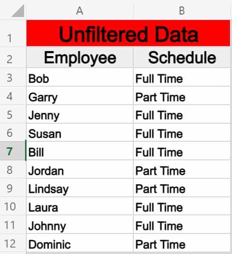
Let’s say that you have a list of employees and their schedule type (Full Time / Part Time) on one tab, and that you want to display a filtered list of full time employees on another tab.
The task: Filter the list of employees on the tab labeled «Filter List», and show a list of employees who have a full time schedule, on a separate tab
The logic: Filter the range ‘Filter List’!A3:B12, where the range ‘Filter List’!B3:B12 is equal to the text «Full Time»
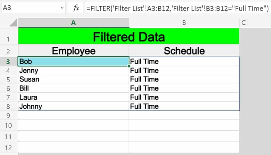
The formula: The formula below, is entered in the blue cell (A3), for this example
=FILTER(‘Filter List’!A3:B12,’Filter List’!B3:B12=»Full Time»)
Here is a list of employees and their schedules, which is held on a tab labeled «Filter List»
And here is a filtered list of employees who have full time schedules, where the filter formula and output data are held on a separate tab.
Pop Quiz: Test your knowledge
Answer the questions below about the Excel FILTER function, to refine your knowledge! Scroll to the very bottom to find the answers to the quiz.
Question #1
Which of the following formulas uses a «cell reference» in the filter condition?
- =FILTER(A1:D15, B1:B15<0.6)
- =FILTER(A2:C15, C2:C15=F1)
- =FILTER(A1:P25, G1:G25=»Yes»)
Question #2
Which of the following formulas uses the «Not Equal» operator?
- =FILTER(C1:T50, J1:J50>100)
- =FILTER(A1:B75, B1:B75=»No»)
- =FILTER(S1:Z100, T1:T100<>»True»)
Question #3
True or False: If the column(s) in the source range and the column in the filter condition are not the same size (if one has more rows than the other), the formula will not work, and will display an error.
- True
- False
Question #4
Which of the following formulas uses AND logic, where BOTH conditions must be met to satisfy the filter criteria?
- =FILTER(C1:F20, (F1:F20=»Yes»)+(E1:E20=»Active»))
- =FILTER(C1:F35, (F1:F35=»Yes»)*(E1:E35=»Active»))
Question #5
Which of the following formulas uses OR logic, where EITHER condition can be met to satisfy the filter criteria?
- =FILTER(A1:K10, (K1:K10=»Yes»)*(J1:J10=»Active»))
- =FILTER(A3:K33, (K3:K33=»Yes»)+(J3:J33=»Active»))
Answers to the questions above:
Question 1: 2
Question 2: 3
Question 3: 1
Question 4: 2
Question 5: 2
Start a new search
To find content from modules and lessons
Overview
How to filter data from a worksheet
Now we will see that we can filter data from a worksheet in MS Excel.
The first thing which we need to check when we want to filter any data is that no row should be empty.
Now we will go to our DATA tab and select ‘Filter’ option, which will bring a dropdown option beside every column, and hence we can select any column which we want to filter and inside it select data according to our requirement.
After doing this it will show us only the filtered data which we selected.
We can also filter our data by providing certain conditions by using ‘filter option’ option. In that we can limit or set our data as our requirement.
See More
In Excel, the FILTER function is used to filter a set of data based on the criteria you define. The function belongs to the Dynamic Arrays category of functions. The output is an array of values that spills into a range of cells automatically, beginning with the cell where you enter a formula.
Filters are used to extract information from a large data set. They are usually used when it is too time-consuming to manually search through the entire dataset. Filters in Excel can be applied to columns or rows. Filtering columns will only show the data that meets the filter criteria in that column, while filtering rows will only show the data that meets the filter criteria in that row.
Setting up a filter in MS Excel is not hard at all. It can be done by following these simple steps:
- Select the cells that you want to filter on.
- Go to Data > Filter > Filter.
- Select the fields you want to filter on, and then click OK.
There are four types of filters:
- AutoFilter
- Quick Filters
- Custom Filters
- Top 10 Filters
- A filter is a powerful tool that allows you to remove data from your dashboard that matches specific criteria.
- You can use it to remove data from a column, row or entire dashboard.
- For example, if you want to remove all the rows where the sales amount is less than $10,000, then you would select the column and enter $10000 in the filter field.
Learner’s Ratings
Reviews
Y
Yash kalra
I dont understood the quiz part the quiz is totally different from the video
S
Sunny kumar
This is a best learning app
K
Kajal Londhe
Best knowledge improve thank you so much
B
Brijesh Yadav
Really thankful to you to explain in such a lucent language
R
RESHMI KUMARI
its very useful for us
S
SHIVAM TIWARI
Formula wala pura uper ja rha
N
Navjeet Kaur
The theory is really good, but practice sheets must also be provided so that we can practice hand to hand. Excel is all about practice more than theory.
A
Aman kesarwani
Hi.
Please mujhe free mai certificate dedo please 😭😥🙏🙏
D
DABLOO Kumar
good and very suficient course
Show More