
![]()
Download Article
![]()
Download Article
Are you new to Microsoft Excel and need to work on a spreadsheet? Excel is so overrun with useful and complicated features that it might seem impossible for a beginner to learn. But don’t worry—once you learn a few basic tricks, you’ll be entering, manipulating, calculating, and graphing data in no time! This wikiHow tutorial will introduce you to the most important features and functions you’ll need to know when starting out with Excel, from entering and sorting basic data to writing your first formulas.
Things You Should Know
- Use Quick Analysis in Excel to perform quick calculations and create helpful graphs without any prior Excel knowledge.
- Adding your data to a table makes it easy to sort and filter data by your preferred criteria.
- Even if you’re not a math person, you can use basic Excel math functions to add, subtract, find averages and more in seconds.
-

1
Create or open a workbook. When people refer to «Excel files,» they are referring to workbooks, which are files that contain one or more sheets of data on individual tabs. Each tab is called a worksheet or spreadsheet, both of which are used interchangeably. When you open Excel, you’ll be prompted to open or create a workbook.
- To start from scratch, click Blank workbook. Otherwise, you can open an existing workbook or create a new one from one of Excel’s helpful templates, such as those designed for budgeting.
-
2
Explore the worksheet. When you create a new blank workbook, you’ll have a single worksheet called Sheet1 (you’ll see that on the tab at the bottom) that contains a grid for your data. Worksheets are made of individual cells that are organized into columns and rows.
- Columns are vertical and labeled with letters, which appear above each column.
- Rows are horizontal and are labeled by numbers, which you’ll see running along the left side of the worksheet.
- Every cell has an address which contains its column letter and row number. For example, the top-left cell in your worksheet’s address is A1 because it’s in column A, row 1.
- A workbook can have multiple worksheets, all containing different sets of data. Each worksheet in your workbook has a name—you can rename a worksheet by right-clicking its tab and selecting Rename.
- To add another worksheet, just click the + next to the worksheet tab(s).
Advertisement
-
3
Save your workbook. Once you save your workbook once, Excel will automatically save any changes you make by default.[1]
This prevents you from accidentally losing data.- Click the File menu and select Save As.
- Choose a location to save the file, such as on your computer or in OneDrive.
- Type a name for your workbook. All workbooks will automatically inherit the the .XLSX file extension.
- Click Save.


Advertisement
-
1
Click a cell to select it. When you click a cell, it will highlight to indicate that it’s selected.
- When you type something into a cell, the input text is called a value. Entering data into Excel is as simple as typing values into each cell.
- When entering data, the first row of your worksheet (e.g., A1, B1, C1) is typically used as headers for each column. This is helpful when creating graphs or tables which require labels.
- For example, if you’re adding a list of dates in column A, you might click cell A1 and type Date into the cell as the column header.
-
2
Type a word or number into the cell. As you’re typing, you’ll see the letters and/or numbers appear in the cell, as well as in the formula bar at the top of the worksheet.
- When you start practicing more advanced Excel features like creating formulas, this bar will come in handy.
- You can also copy and paste text from other applications into your worksheet, tables from PDFs and the web.
-
3
Press ↵ Enter or ⏎ Return. This enters the data into the cell and moves to the next cell in the column.
-
4
Automatically fill columns based on existing data. Let’s say you want to make a list of consecutive dates or numbers. Or what if you want to fill a column with many of the same values that follow a pattern? As long as Excel can recognize some sort of pattern in your data, such as a particular order, you can use Autofill to automatically populate data into the rest of your column. Here’s a trick to see it in action.
- In a blank column, type 1 into the first cell, 2 into the second cell, and then 3 into the third cell.
- Hover your mouse cursor over the bottom-right corner of the last cell in your series—it will turn to a crosshair.
- Click and drag the crosshair down the column, then release the mouse button once you’ve gone down as far as you like. By default, this will fill the remaining cells with the value of the selected cell—at this point, you’ll probably have something like 1, 2, 3, 3, 3, 3, 3, 3.
- Click the small icon at the bottom-right corner of the filled data to open AutoFill options, and select Fill Series to automatically detect the series or pattern. Now you’ll have a list of consecutive numbers. Try this cool feature out with different patterns!
- Once you get the hang of AutoFill, you’ll have to try flash fill, which you can use to join two columns of data into a single merged column.
-
5
Adjust the column sizes so you can see all of the values. Sometimes typing long values into a cell hides the value and displays hash symbols ### instead of what you’ve typed. If you want to be able to see everything, you can snap the cell contents to the width of the widest cell. For example, let’s say we have some long values in column B:
- To expand the contents of column B, hover the cursor over the dividing line between the B and C at the top of the worksheet—once your cursor is right on the line, it will turn to two arrows pointing in either direction.[2]
- Click and drag the separator until the column is wide enough to accommodate your data, or just double-click the separator to instantly snap the column to the size of the widest value.
- To expand the contents of column B, hover the cursor over the dividing line between the B and C at the top of the worksheet—once your cursor is right on the line, it will turn to two arrows pointing in either direction.[2]
-
6
Wrap text in a cell. If your longer values are now awkwardly long, you can enable text wrapping in one or more cells. Just click a cell (or drag the mouse to select multiple cells), click the Home tab, and then click Wrap Text on the toolbar.
-
7
Edit a cell value. If you need to make a change to a cell, you can double-click the cell to activate the cursor, and then make any changes you need. When you’re finished, just press Enter or Return again.
- To delete the contents of a cell, click the cell once and press delete on your keyboard.
-
8
Apply styles to your data. Whether you want to highlight certain values with color so they stand out or just want to make your data look pretty, changing the colors of cells and their containing values is easy—especially if you’re used to Microsoft Word:
- Select a cell, column, row, or multiple cells at once.
- On the Home tab, click Cell Styles if you’d like to quickly apply quick color styles.
- If you’d rather use more custom options, right-click the selected cell(s) and select Format Cells. Then, use the colors on the Fill tab to customize the cell’s background, or the colors on the Font tab for value colors.
-
9
Apply number formatting to cells containing numbers. If you have data that contains numbers such as prices, measurements, dates, or times, you can apply number formatting to the data so it will display consistently.[3]
By default, the number format is General, which means numbers display exactly as you type them.- Select the cell you want to format. If you’re working with an entire column or row, you can just click the column letter or row number to select the whole thing.
- On the Home tab, click the drop-down menu at the top-center—it’ll say General by default, unless you selected cells that Excel recognizes as a different type of number like Currency or Time.
- Choose one of the formatting options in the list, such as Short Date or Percentage, or click More Number Formats at the bottom to expand all options (we recommend this!).
- If you selected More Number Formats, the Format Cells dialog will expand to the Number tab, where you’ll see several categories for number types.
- Select a category, such as Currency if working with money, or Date if working with dates. Then, choose your preferences, such as a currency symbol and/or decimal places.
- Click OK to apply your formatting.


Advertisement
-
1
Select all of the data you’ve entered so far. Adding your data to a table is the easiest way to work with and analyze data.[4]
Start by highlighting the values you’ve entered so far, including your column headers. Tables also make it easy to sort and filter your data based on values.- Tables traditionally apply different or alternating colors to every other row for easy viewing. Many table options also add borders between cells and/or columns and rows.
-
2
Click Format as Table. You’ll see this at the top-center part of the Home tab.[5]
-
3
Select a table style. Choose any of Excel’s default table styles to get started. You’ll see a small window titled «Create Table» once selected.
- Once you get the hang of tables, you can return here to customize your table further by selecting New Table Style.
-
4
Make sure «My table has headers» is selected and click OK. This tells Excel to turn your column headers into drop-down menus that you can easily sort and filter. Once you click OK, you’ll see that your data now has a color scheme and drop-down menus.
-
5
Click the drop-down menu at the top of a column. Now you’ll see options for sorting that column, as well as several options for filtering all of your data based on its values.
-
6
Choose which data to display based on values in this column. The simplest way to do this is to uncheck the values you don’t want to display—if you uncheck a particular date, for example, you’ll prevent rows that contain the selected date in from appearing in your data. You can also use Text Filters or Number Filters, depending on the type of data in the column:
- If you chose a numerical column, select Number Filters, then choose an option like Greater Than… or Does Not Equal to be extra specific about which values to hide.
- For text columns, you can choose Text Filters, where you can specify things like Begins with or Contains.
- You can also filter by cell color.
-
7
Click OK. Your data is now filtered based on your selections. You’ll also see a small funnel icon in the drop-down menu, which indicates that the data is filtering out certain values.
- To unfilter your data, click the funnel icon, click Clear filter from (column name), and then click OK.
- You can also filter columns that aren’t in tables. Just select a column and click Filter on the Data tab to add a drop-down to that column.
-
8
Sort your data in ascending or descending order. Click the drop-down arrow at the top of a column to view sorting options—these allow you to sort all of your data in order based on the current column.
- If you’re working with numbers, click Smallest to Largest to sort in ascending order, or Largest to Smallest for descending order.[6]
- If you’re working with text values, Sort A to Z will sort in ascending order, while Sort Z to A will sort in reverse.
- When it comes to sorting dates and times, Sort Oldest to Newest will sort with the earliest date at the top and the oldest date at the bottom, and Newest to Oldest displays the dates in descending order.
- When you sort a column, all other columns in the table adjust based on the sort.
- If you’re working with numbers, click Smallest to Largest to sort in ascending order, or Largest to Smallest for descending order.[6]


Advertisement
-
1
Select the data in your worksheet. Excel’s Quick Analysis feature is the easiest way to perform basic calculations (including totals, averages, and counts) and create meaningful tables or graphs without the need for advanced Excel knowledge.[7]
Use your mouse to select your data (including your column headers) to get started. -
2
Click the Quick Analysis icon. This is the small icon that pops up at the bottom-right corner of your selection. It looks like a window with some colored lines.
-
3
Select an analysis type. You’ll see several tabs running along the top of the window, each of which gives you different option for visualizing your data:
- For math calculations, click the Totals tab, where you can select Sum, Average, Count, %Total, or Running Total. You’ll be able to choose whether to display the results at the bottom of each column or to the right.
- To create a chart, click the Charts tab, then select a chart to visualize your data. Before you settle on a chart, just hover the cursor over each option to see a preview.
- To add quick chart data to individual cells, click the Sparklines tab and choose a format. Again, you can hover the cursor over each option to see a preview.
- To instantly apply conditional formatting (which is usually a little more complex in Excel) based on your data, use the Formatting tab. Here you can choose an option like Color or Data Bars, which apply colors to your data based on trends.


Advertisement
-
1
Quickly add data with AutoSum. AutoSum is a built-in Excel function that makes it easy to find the total of one or more columns in a few clicks. Functions or formulas that perform calculations and other tasks based on the values of cells. When you use a function to get something done, you’re creating a formula, which is like a math equation. If you have a column or row of numbers you want to add:
- Click the cell below the numbers you want to add (if a column) or to the right (if a row).[8]
- On the Home tab, click AutoSum toward the upper-right corner of the app. A formula beginning with =SUM(cell+cell) will appear in the field, and a dotted line will surround the numbers you’re adding.
- Press Enter or Return. You should now see the total of the numbers in the selected field. This is here because you created your first formula—which you didn’t have to write by hand!
- If you change any numbers in your data after using AutoSum, the AutoSum value will update automatically.
- Click the cell below the numbers you want to add (if a column) or to the right (if a row).[8]
-
2
Write a simple math formula. AutoSum is just the beginning—Excel is famous for its ability to do all sorts of simple and complex math calculations on data. Fortunately, you don’t have to be a math whiz to create simple formulas to create everyday math formulas, like adding, subtracting, and multiplying. Here’s some basic formulas to get you started:
-
Add: — Type =SUM(cell+cell) (e.g.,
=SUM(A3+B3)) to add two cells’ values together, or type =SUM(cell,cell,cell) (e.g.,=SUM(A2,B2,C2)) to add a series of cell values together.- If you want to add all of the numbers in a whole column (or in a section of a column), type =SUM(cell:cell) (e.g.,
=SUM(A1:A12)) into the cell you want to use to display the result.
- If you want to add all of the numbers in a whole column (or in a section of a column), type =SUM(cell:cell) (e.g.,
-
Subtract: Type =SUM(cell-cell) (e.g.,
=SUM(A3-B3)) to subtract one cell value from another cell’s value. -
Divide: Type =SUM(cell/cell) (e.g.,
=SUM(A6/C5)) to divide one cell’s value by another cell’s value. -
Multiply: Type =SUM(cell*cell) (e.g.,
=SUM(A2*A7)) to multiply two cell values together.
-
Add: — Type =SUM(cell+cell) (e.g.,


Advertisement
-
1
Select a cell for an advanced formula. What if you need to do something more complicated than just adding numbers? Even if you don’t know how to write formulas by hand, you can still create useful formulas that work with your data in various ways. Start by clicking the cell in which you want to display your formula.
-
2
Click the Formulas tab. It’s a tab at the top of the Excel window.
-
3
Explore the Function Library. Several function categories appear in the toolbar, such as Financial, Text, and Math & Trig. Click the options to check out the types of functions available, though they might not make a whole lot of sense just yet.
-
4
Click Insert Function. This option is in the far-left side of the Formulas toolbar. This opens the Insert Function window, which gives you a more detailed breakdown of each function.
-
5
Click a function to learn about it. You can type what you want to do (such as round), or choose a category to filter the list of functions. Then, click any function to read a description of how it works and view its syntax.
- For example, to select the formula for finding the tangent of an angle, you would scroll down and click the TAN option.
-
6
Select a function and click OK. This creates a formula based on the selected function.
-
7
Fill out the function’s formula. When prompted, type in the number or select a cell for which you want to use the formula.
- For example, if you select the TAN function, you’ll type in the number for which you want to find the tangent, or select the cell that contains that number.
- Depending on your selected function, you may need to click through a couple of on-screen prompts.
-
8
Press ↵ Enter or ⏎ Return to run the formula. Doing so applies your function and displays it in your selected cell.


Advertisement
-
1
Set up the chart’s data. If you’re creating a line graph or a bar graph, for example, you’ll want to use one column of cells for the horizontal axis and one column of cells for the vertical axis. The best way to do this is to place your data in a table.
- Typically speaking, the left column is used for the horizontal axis and the column immediately to the right of it represents the vertical axis.
-
2
Select the data in your table. Click and drag your mouse from the top-left cell of the data down to the bottom-right cell of the data.
-
3
Click the Insert tab. It’s a tab at the top of the Excel window.
-
4
Click Recommended Charts. You’ll find this option in the «Charts» section of the Insert toolbar. A window with different chart templates will appear.
-
5
Select a chart template. Click the chart template you want to use based on the type of data you’re working with. If you don’t see a chart type you like, click the All Charts tab to explore by category, such as Pie, Bar, and X Y Scatter.
-
6
Click OK. It’s at the bottom of the window. This creates your chart.
-
7
Use the Chart Design tab to customize your chart. Any time you click your chart, the Chart Design tab will appear at the top of Excel. You can adjust the chart style here, change colors, and add additional elements.
-
8
Double-click a chart element to manage it in the Format panel. When you double-click something on your chart, such as a value, line, or bar, you’ll see options you can edit in the panel on the right side of excel. Here you can change the axis labels, alignment, and legend data.


Advertisement
Add New Question
-
Question
How do you add a check mark or an X mark to a cell?

You can go into Insert, then Symbol, and choose the symbol you want. After that, you can just copy and paste the symbol from one cell to another.
-
Question
Can I add work sheets on Excel?
Yes. At the bottom left of the Excel you will see the list of sheets. To the left of those sheets you will find a «+» sign. Click on it.
-
Question
How do I move cell contents to another cell?
Highlight the cell, right-click, and click Copy. Click destination cell, right-click and Paste.
See more answers
Ask a Question
200 characters left
Include your email address to get a message when this question is answered.
Submit
Advertisement
Video
Thanks for submitting a tip for review!
References
About This Article
Article SummaryX
1. Purchase and install Microsoft Office.
2. Enter data into individual cells.
3. Format cells based on certain criteria.
4. Organize data into rows and columns.
5. Perform math operations using formulas.
6. Use the Formulas tab to find additional formulas.
7. Use data to create charts.
8. Import data from other sources.
Did this summary help you?
Thanks to all authors for creating a page that has been read 646,684 times.
Reader Success Stories
-

«I am applying for a job that requires comprehensive knowledge of Excel. Well, I don’t have it, but this article…» more
Is this article up to date?
How do you use Excel? We want to show you a quick Excel guide in this article on how to use Excel for beginners.
We especially appeal to anyone who has never used Excel before and wants to know the first steps on how to use Excel.
If you already know Excel, then this article is not for you.
The goal is to offer you an Excel guide for beginners to introduce you to the spreadsheet and show you what you can do.
In this guide, you will learn the following
Welcome to Excel
For beginners, Excel might be a little scary. It’s normal!
What is Excel for?
Microsoft Excel is a helpful and powerful application for data analysis and documentation. It is a spreadsheet program, which includes a number of columns and rows, where each intersection of a column and a row is a “cell.” Moreover, each cell contains one point of data or one piece of information.
So, you can make information more comfortable to find by organizing the information in this way, and you can automatically draw information from changing data.
Using formulas and functions, you can make sense of your data by turning it into useful information. For example, you can automatically view sums, averages, and totals.
Excel-workbooks VS worksheets
Workbooks: Excel documents are called workbooks, and many (not all) versions of Excel will automatically have three tabs, each with its own blank worksheet when you first create an Excel document (a workbook).
If that’s not what your version of Excel does, don’t worry, we’ll learn how to build them.
Worksheets: The worksheets are the actual components where the data is entered. Think of the worksheets as those tabs if it is easy to think of it visually.
By right-clicking and choosing the delete option, you can add tabs or remove tabs. Those worksheets are the real spreadsheets we are dealing with and finally, we are stored in the workbook file.
What will you learn in this article?
It’s a short path for beginners where you’ll learn how to use Excel, such as- what a spreadsheet is, how to enter data and save, print, share your Workbook.
To get started with Excel, that is all you need to remember.
What about the rest? Look for a solution in this blog: you will find many interesting articles that will allow you to learn many features.
Excel is a powerful application, even if sometimes it might be a little bothering. Nothing serious, we assure you!
That’s why we thought of this quick guide for those who want to start using Excel.
The secret to knowing Excel is:
- Have a lot of willpower and desire to learn,
- Do a lot of practice and,
- Have a good teacher!
On my computer, I have installed the version of Excel 2019 for Windows. If you have a different version, no problem! The steps are identical.
When you first open Excel, the application will ask you what you want to do. It will show you a similar window.
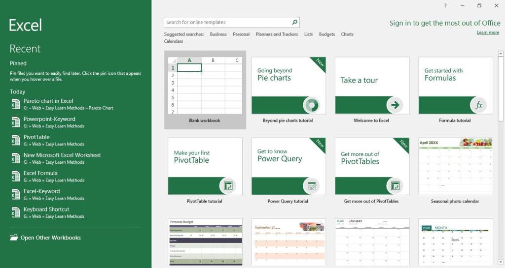
To open a new workbook, click Blank Workbook.
If you want to open an existing workbook instead, click Open. Then select the file in the list or click Browse.

At this point, through the dialog box, find the Workbook you are looking for, select it, and click Open or double click on the selected Workbook.

You just heard of Workbook.
In Excel, the Workbook is a file. It usually has an extension of type . XLSX, but it could be . XLS if you are using a version older than Excel 2007.
I anticipate that you will also hear about Worksheets.
A worksheet is a single sheet within a workbook. A workbook can contain many sheets. So each Excel sheet is identified by a label and name that you will find at the bottom of the screen.
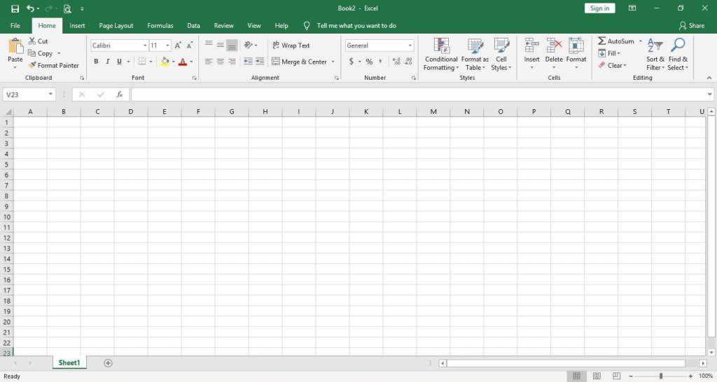
How to use excel for beginners: the ribbon

The ribbon is the control panel of Excel. Inside you will find many Cards, Groups, and Commands. You can do pretty much anything you want right from the ribbon.
Find the ribbon at the top of the window.

There are several tabs, including Home, Insert, Page Layout, Formulas, etc.
Each tab contains groups of commands. For example, you will find the Clipboard, Font, Alignment, Numbers, Styles, Cells, Editing group, all with different buttons on the Home tab.
Try clicking on the tabs to see what groups and buttons are contained within them.
Finally, you will find a search bar that says, “What do you want to do?”. Please enter in it what you are searching for, and Excel will help you find it. This is especially useful when looking for something specific – you can’t go through all the buttons to find out what they do.
How to use excel for beginners: Worksheets
As mentioned above, a workbook can contain multiple sheets. By default, Excel contains only one worksheet, but you can insert more.
Click on a label to open that particular worksheet.

To add a new worksheet, click the button at the end of the sheet list. The button with the “+” symbol.
Also, you can reorder the sheets in your Workbook by simply dragging them to a new location.
And if you right-click on a sheet label, you’ll get a context menu with a number of options. Among these, Rename and Delete are the most useful. For now, you can leave out the rest.

How to insert data into Excel
It’s time to enter some data!
Data entry is one of the most essential and simple things you can do in Excel.
So just click in an empty cell and start typing.
Type the following numbers into the cells.

Excel cells can contain- text, numbers, and formulas.
Try typing some text or date in any cell and see what happens.
There are many other ways to enter data within a worksheet. For the moment, we will limit ourselves to this. However, we will use the numbers just entered to try to do the math.
Apply cell borders
- Select the cell or range of cells to which you want a border to be added.
- On the Home tab, click the arrow next to Borders in the Font group, and then click the border style you like.

Apply Fill and Font Color
- Select the cell or range of cells to which you want cell coloring to be applied.
- Click the arrow next to the Fill Color Button symbol on the Home tab in the Font group, and then, under Theme Colors or Standard Colors, select the color you want.

- To change the font color, click the Font Color button symbol on the Home tab in the Font group, then select the color you want under Theme Colors or Standard Colors.

How to include the data in a table
Putting the data into a table is an easy way to access the power of Excel.
- To select the data, click the first cell and dragging it to the last cell in your data. To use the keyboard to select your data, click the first cell, hold down the Shift key, and press the last cell’s arrow keys.
- After selecting your data, a Quick Analysis button
 appears in the bottom-right corner and clicks on it.

- Move your cursor to the Table button in the Quick Analysis Table gallery, and then click the Table button.

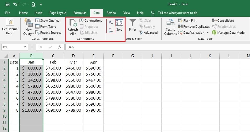
How to use excel for beginners: Sort
To quickly sort your Data
- Choose a date range, such as A1:E9 (Multiple columns and rows) or B Cell (single column). Titles you have created to define columns or rows can be included in the range.
- Select a single cell in the column that you want to sort.
- In Excel, click the A to Z
 command to sort A to Z or the smallest number to the largest (A to Z or the smallest number to the largest) to perform an ascending sort.
- In Excel, click the Z to A command to sort Z to A or the largest number to the smallest number (Z to A or the largest number to the smallest) to perform a descending sort.
To sort by the specific situation
- Firstly, select a single cell from anywhere in the range to be sorted.
- Choose Sort on the Data tab, in the Sort & Filter group.
- The Sort dialog box becomes visible.
- In the Sort By list, select the first column you want to sort from.
- Select any Values, Cell Color, Font Color, or Cell Icon from the Sort On the list.
- In the Order list, pick the alphabetically or numerically ascending or descending (— for example, A to Z or Z to A for text or lower to higher or higher to lower for numbers) order that you want to add to the sort operation.
How to filter your Excel data
- Select the data to be filtered.

- In the Data tab, click Filter in the Sort & Filter group.
- On the Data tab, group Sort, and Filter.
- Click the Arrow Filter drop-down arrow in the column header to show a list of filtering choices that you can make.

- To select by value, clear the check box (Select All) in the list. This removes from all checkboxes the checkmarks. Then pick only the values you want to see, and then click OK to see the results.
How to use excel for beginners: do the basic calculations
Now that we have seen how to insert some data into a worksheet, let’s see how to do some simple processing.
Performing basic calculations in Excel is simple.
The important thing that you must ALWAYS keep in mind when working with formulas is that: all formulas always start with an equal sign.
Whenever you perform a calculation, the first thing you need to type is the equal sign “=”.
This is the way to alert Excel to prepare to perform a calculation.
Now let’s try to do a sum in Excel. Type the following formula in cell A3.
=10+7
Then, hit the Enter key.
Excel evaluates your formula and displays the result: 17.

Now, look at the formula bar. You will see the original formula.
This is useful in case you forget what you originally typed.
You can modify the contents of a cell in the formula bar as well.
Click in any cell, then go to the formula bar and start typing.
Perform subtraction, multiplication, and division are just as easy.
Enter the following formulas in cells B3, C3, and D3, respectively.

The result will be the following.

Now let’s change perspective and try something different. What I’m going to show you is one of the fundamentals of Excel.
Type the same data into another worksheet. Now click in cell A3 and type the following:
=A1+A2
Finally, hit the Enter key.
You should get 17: the sum of the numbers in cells A1 and A2.
At this point, change one of the numbers to A1 or A2.
What happens when you change the values in one of the cells? You will notice that Excel automatically updates the total.
Try applying the different arithmetic operations in the other cells. The result will be identical, but the perspective is distorted.

Subsequently, it will be sufficient to change the cells’ contents to which the formula refers to obtain different results.
What you did manually earlier can be done automatically.
Use AutoSum to add your Data
When you’ve entered numbers in your sheet, you may want to add them up. A quick way to do that is by using AutoSum.
- Select the cell below or to the right of the numbers that you want to add.
- Click the Home tab, and then in the Editing group, click AutoSum.
- On the Home tab, AutoSum.

- AutoSum adds up the numbers and finally displays the result in the selected cell.
The heart of Excel: the functions
The engine of Excel functions. Thanks to the functions, you can perform complex calculations.
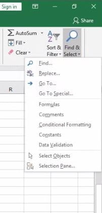
Basically, you will find the standard Excel functions in the Edit group of the Home tab.

Now let’s see how to use one of the many Excel functions.
Let’s go back to the sheet containing the data entered previously.
Let’s go to cell E1 and then click on the Excel Sum function.
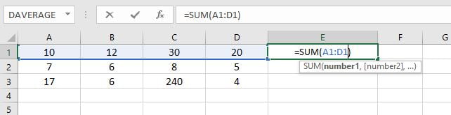
Then, hit the Enter key.
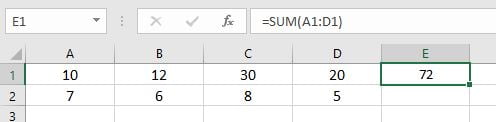
The resulting number, 72, is the sum of the numbers in cells A1, B1, C1, and D1.
As you can see, in the SUM function, I entered the word “A1: D1”.
This writing tells Excel to refer to all cells A1 to D1.
There are many useful functions in Excel. Some you can use alone, others instead as nested functions. Nested functions are functions within functions.
If you want to see all the functions that are available, then go to the Formulas tab, and you will find all the function libraries.

Then, click on one of the icons to find the function that will allow you to solve a specific problem.
Scroll through the list of functions that are available and pick the one you want.
When you start typing a formula (don’t forget to enter the equal sign ), Excel will help by showing you some of the possible functions you might be looking for.

Finally, after typing a formula name and the opening parenthesis, Excel will tell you which arguments you need to enter.

It might not be easy-to-understand Excel’s advice if you’ve never used a function before. It will become clearer, however, with a little practice and experience.
How to use excel for beginners: Save your work
In order not to lose the work you’ve done within your Workbook, you’ll need to save your changes.

Use the F12 function key to save. If you haven’t saved your file yet, Excel will ask you where you want to save it and what name you want to assign.
On the other hand, you can click the button Save this in the Quick Access toolbar.
![]()
I suggest you save often.
Get into the habit of naming and choosing a location to save your file before you start working.
Otherwise, losing your job could be painful!
How to use excel for beginners: Print worksheet
- Click the File tab, and then the Print button, or keyboard shortcut press Ctrl+P.
- By clicking the Next Page and Previous Page arrows, preview the pages.
- In the Print Preview window, the Next and Previous buttons.
- Basically, depending on the settings of your printer, the preview window shows the pages in black and white or in color.
- You can change page margins or add page breaks when you don’t like how your pages are written.

- Finally, click Print.
How to use excel for beginners: Share workbook
The easiest way to share your Excel files is to use OneDrive.
Simply click the Share button in the top right corner of the window.
Excel will guide you through sharing the document.

Also, you can save your document and send it by email.
On the other hand, you can use any other cloud service (Such as- IDrve, SugarSync, Dropbox, etc.) to share it with whoever you want.
Activate and use an add-ins
- Choose Options on the File tab and then choose the Add-Ins category.
- Near the bottom of the Excel Options dialog box, in the Manage box, make sure that Excel Add-ins are selected, then click Go.
- In the Add-Ins dialog box, select the add-ins you want to use in the check boxes, and then click OK.

If Excel shows a message stating that this add-in cannot be run and prompts you to install it, finally click Yes to install add-ins.
How to center text across cells without using the Merge and Center option in Excel?
It’s not difficult to do this, go to your Excel sheet and select the cells that you want to center.
After selection, right-click on it and select Format Cells or use the keyboard shortcut Ctrl+1 then you will see the Format Cells dialog box.
Go to Alignment in the dialog box.
Choose Center Across Selection from Horizontal group.
And finally, click OK.
This is a beginners guide to Excel spreadsheets
A “Dummies” Guide to Excel for Beginners
Welcome to our free Excel for beginners guide! In this guide, we will give you everything a beginner needs to know – what is Excel, why do we use it, and what are the most important keyboard shortcuts, functions, and formulas. If you’re new to MS Excel, then you’ve come to the right spot and our dummies guide to Excel will give you the foundation you’re looking for.
Launch our free YouTube course on Excel for beginners below!
What is Excel?
The Microsoft Excel program is a spreadsheet consisting of individual cells that can be used to build functions, formulas, tables, and graphs that easily organize and analyze large amounts of information and data.
Excel works like a database, organized into rows (represented by numbers) and columns (represented by letters) that contain information, formulas, and functions used to perform complex calculations.
The first version of Excel was released by Microsoft in 1985, and by the 1990’s it was one of the most widely used and important business tools in the world.
Today, Excel is still a ubiquitous program, found on just about every personal and business computer on the planet.
Launch our free Excel crash course. The best way to learn is by doing, which is why our FREE step by step tutorial on how to use Excel is the most efficient way to learn with your own spreadsheet.
Why do we use Excel?
Simply put, Excel is the easiest way to organize and manage financial information, which is why most businesses use it extensively. If offers total flexibility and customization in the way it’s used.
Another reason to use Excel is that it’s so accessible. With virtually zero training or experience, a user can open up a workbook, start inputting data and begin calculating and analyzing information.
Here are the top 5 reasons we use Excel:
- To organize financial data
- To organize contact information
- To organize employee information
- To organize personal information
- To be a calculator
What are the most important functions?
There are hundreds of formulas and combinations of formulas that can be used in Excel spreadsheets, but since this is an Excel for beginners guide, we have narrowed it down to the most important and most basic ones. We cover all of these functions and more in our Free Excel Crash Course.
The most important functions include:
- =SUM() – adds a series of cells together
- =AVERAGE() – calculates the average of a series of cells
- =IF() – checks if a condition is met and returns a value if YES and a value if NO
- =MIN() – returns the minimum value in a series
- =MAX() – returns the maximum value in a series
- =LARGE() – returns the k-th largest value in a series
- =SMALL() – returns the k-th smallest value in a series
- =COUNT() – counts the number of cells in a range that contain numbers
- =VLOOKUP() – looks for a value in the leftmost column of a table and returns in the same row from a column you specify
Here is a more detailed list of Excel formulas and functions. We recommend familiarizing yourself with all of them to become a proficient user.
What are the most important shortcuts?
If you use Excel frequently it’s important to be able to work as quickly as possible. Using Excel shortcuts is the best way to speed up your skills. By avoiding using the mouse, you can save cut down on the time it takes to click through each step of a procedure. Keyboard shortcuts are much faster and allow the user to move around the spreadsheet much more efficiently.
The most important Excel shortcuts include:
- F2 Edit active cell
- F4 Toggle references
- CTRL + 1 Format Cells
- CTRL + C Copy
- CTRL + V Paste
- CTRL + R Fill right
- CTRL + D Fill down
- ALT + = Auto Sum
- ALT, I, R Insert row
- ALT, I, C Insert column
Keyboard Shortcuts Sheet
Looking to be an Excel wizard? Increase your productivity with CFI’s comprehensive keyboard shortcuts guide.
How can I get better at Excel?
In order to improve your Excel skills, you need to practice. It’s not enough to simply read the functions and formulas in an article like this, you also have to watch and learn from the power users. Many of the functions and formulas, sadly, are not intuitive or obvious, so you’ll need to go over them many times on your own before they become natural for you.
Check out our free spreadsheet formulas course to watch an Excel power user in action!
After you’ve taken the course, try recreating everything on your own from scratch, and see if you can remember all of the formulas and functions.
What jobs use Excel spreadsheets?
There are many jobs that use Excel on a daily basis. In fact, it’s hard to think of a job that doesn’t use this program. Even though technology has changed the way we work in many careers, Excel has remained as one of the few tools that are so simple and powerful that it seems to remain no matter what other software comes out.
Just about every office job requires Excel. The broad categories of careers that use Excel are:
- Finance and accounting
- Marketing and social media
- Human Resources
- Operations
- Technology
At CFI we specialize in finance and accounting roles, so in our universe of jobs, there are many different careers that use Excel.
Explore our interactive career map to learn more about finance jobs beyond our dummies guide to Excel for beginners.
Some of the most common finance jobs that use Excel are:
- Investment banking
- Equity research
- Corporate banking
- Private equity
- Corporate development
- Investor Relations
What else do I need to know about Excel?
Hopefully, this Excel for beginners guide has given you a good start. Our free Excel crash course would be a great next step for you!
The best way to learn is to open up a new workbook and try using all the formulas and functions we’ve given you in your own spreadsheet.
Once you’re comfortable with the material in this article, take a look at the free crash course below and you’ll be a power user in no time. You can also check out some intermediate level Excel tips and formulas.
If you prefer to learn by reading, there are plenty of Excel books that are highly regarded. The Excel Bible by John Walkenback is an extremely comprehensive book that you may want to consider.
More Excel guides
If you liked our guide to Excel for beginners we think you’ll love these helpful CFI resources as well. Since the key to becoming great at Excel is lots of practice, we highly recommend you explore these additional resources to expand your knowledge and move past the introductory level. The return on the investment of your time spent will be well worth it!
Our most popular resources include:
- All Excel courses
- Excel templates
- Formulas list
- Shortcuts list
- Excel courses
- Advanced Excel formulas
- See all Excel resources
This is your ultimate guide to excel for beginners.
Excel is a powerful, yet complex program. But it can also be intimidating for beginners.
This blog post gives you an easy-to-follow tutorial with tips and tricks to get you started with Microsoft Excel.
In it, you’ll learn
- The important basics about Excel
- More advanced techniques to make sure you’re getting everything right
- Important Excel shortcuts
What Is Microsoft Excel? What Is It Used For?
Excel was created in the mid-80s as a spreadsheet program for businesses to use to do their accounting and organize data.
Excel is now owned by Microsoft, and it’s been more available than ever with standalone versions, as well as part of the Office suite and Microsoft 365 subscriptions.
Excel can be used across various platforms (desktop, online, or via mobile app), and comes with a library of built-in tools and features that can accomplish nearly anything.
Excel is so powerful that it’s widely used by businesses and professionals everywhere to analyze data, manage financial spreadsheets, and organize information.
Excel can be used for personal or professional reasons. Businesses of any size can get help with payroll, inventory, taxes, finance management, and more.
Home users, you can create budgets, make checklists, keep track of expenses, monitor your weight, and much more!
If you use a computer, chances are you will benefit from incorporating Excel into your daily life.
Using this guide, you can lay down the foundation needed to become a more organized and efficient person with the help of Microsoft Excel.
The Basics of Excel
Excel uses a spreadsheet system that allows you to input numbers, formulas, text, and other visual elements. When you start a new project, you create what’s called a workbook.
In a workbook, you can create and store up to 255 individual sheets. Each sheet is broken down into cells, sorted into columns and rows.
Excel’s Formulas
The formulas in Excel allow you to quickly perform accurate calculations using your data cells. No more doing math in your head — Excel can take care of it for you.
With a wide range of formulas, it can be hard to know which ones you should memorize first to efficiently work with your data.
If you’re just getting started with Excel and want something easy to get the hang of quickly, depend on these simple formulas!
- Start the formula with an equal sign (=) — Before you can start typing any of the formulas below, you need to type an equal sign into the output cell. This will signal Excel that you’re typing a formula.
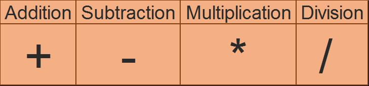
- Addition — Quickly add two cells together with the plus sign (+). For example, if you want to add the value of the A3 and B3 cells together, you’d type “=A3+B3”.
- Subtraction — Similarly, you can subtract the value of a cell from another cell using the hyphen (—). For example, if you want to deduct the value of the A3 cell from the B3 cell, you’d type “=B3-A3”.
- Multiplication — Multiply the values of cells using the asterisk symbol (*). For example, if you want to multiply the A3 cell by 5, you’d use the “=A3*5” formula.
- Division — To divide the values of two or more cells, use the slash sign (/). For example, to divide A3 with B3, you’d use “=A3/B3”.
Formulas can be used with cells in your sheet, and with numbers not bound to the sheet as well. For example, you can add any value to an already existing cell, or add the values of two cells together with the addition formula.
Important Excel Functions
Excel functions can save you time and energy when doing tasks such as adding up cells. The SUM function is a good example of this, which does not require the use of an additional + sign to add together all your numbers in one place.
There are other great functions that do other types of calculations for you too!
The list is endless when it comes down to what complex functions one might need in Excel.
However, if you’re just starting out, here are some that will help ease into understanding them as well as save time.
- SUM — The SUM function is used to find out the sum of values from a group of columns or rows. When used, it will add up all of the values from the specified range. Syntax: =SUM(Cell1:Cell2).
- AVERAGE — The AVERAGE function can be used to calculate the average value of any number of cells. Syntax: =AVERAGE(Cell1:Cell2).
- IF — The IF function tests for a logical condition. If that condition is true, it will return the value. Syntax: =IF(logical_test, [value_if_true], [value_if_false]).
- VLOOKUP — VLOOKUP is a function in Excel that makes it search for a certain value in one column and return a value from another column. Syntax: =VLOOKUP(value, table, col_index, [range_lookup]).
- CONCATENATE — The CONCATENATE function allows you to combine data from multiple cells into one cell. For example, you can combine first names and last names. Syntax: =CONCATENATE (text1, text2, [text3], …).
- AND — The AND function checks if something is true or false. It can check more than two things if you separate the values with a comma. Syntax: =AND(logical1, [logical2], …).
- INDEX — The INDEX function returns the value at a given location in a range or array. You can use it to find individual values, or entire rows and columns. Syntax: =INDEX (array, row_num, [col_num], [area_num]).
There are hundreds of other functions in Excel, but you can’t possibly memorize them all on your first day.
Make sure to keep your brain trained every day by repeating core functions and learning about new ones. Microsoft often sneaks in a couple of new functions with each Excel upgrade as well.
Excel Tips and Tricks for Beginners
Now that you know the basics, we can get into some techniques that’ll make your life much easier when working in Excel.
Make Use of the Quick Access Toolbar
Easily one of the most popular Excel features is the Quick Access toolbar. Excel veterans that have been using the app for years shouldn’t be hesitant to use this feature either.
It speeds up your workflow and allows you to use your favorite tools with ease.
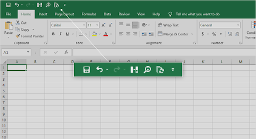
The Quick Access toolbar is located in the top-left of the Excel window
To get started, when you find a command you don’t want to forget about, right-click it and select Add to Quick Access Toolbar.
Now, it’ll be readily available from the toolbar without navigating through menu after menu in the Ribbon.
Use Filters to Sort and Simplify Your Data
Data can be overwhelming when you are looking at a lot of it. It’s easy to get lost in a sea of data. Filters are your map back out!
Filters help you see only certain cells or rows with specific criteria. It’s an easy way for you to choose which records you’re interested in seeing.
This helps make things easier, rather than forcing you to scroll endlessly until you find the desired result set!
There are rows and columns, with filters being the arrows that point you towards what you want. You can filter by column or cell, so there is no limit on how much information will fit into those little cells.
Remove Duplicate Cells
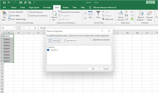
There’s always room for error when manually entering data — or even when a computer does it for you.
It’s important to review your sheets and eliminate any duplicate data when its presence is not appropriate in the sheet. Excel has a special tool for identifying duplicates that you can use.
Removing duplicate entries in Excel
All you have to do is select the Data tab from the Ribbon, then click on the Remove Duplicates button under Tools.
A new window will appear where you can confirm the data you want to work with. Voila!
Fill Data With AutoFill
Did you know that Excel allows you to use predictive technology to your advantage?
Excel can actually ‘learn’ what you usually fill in and provide suggestions based on that information for your next cell automatically.
This Excel feature is called AutoFill, which automatically fills out data if Excel thinks it knows what you’re typing or inputting into the blank space.
AutoFill is located on Excel’s Data tab under Tools. You just have to select the cell you want Excel to fill out for you and click on the AutoFill button.
Excel will then show four or five choices of what Excel thinks is being input into your blank cell.
Add Visual Impact With Conditional Formatting
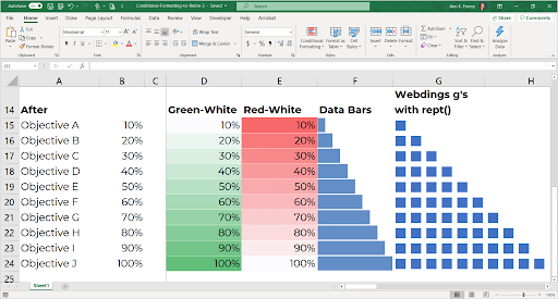
Get information about your sheet at a glance. Conditional formatting separates values based on conditions and fills them with different colors to help you distinguish them.
Excel’s conditional formatting has several rules you can apply to format the data in any way you want.
Conditional formatting is a powerful tool for the clever spreadsheet creator.
The color-coded cells can help you to make sense of your data at a moment’s glance, and they’re even customizable! Whether it be creating custom rules or altering colors, conditional formatting will never let your spreadsheets look boring again.
Quickly Insert Screenshots
Newer versions of Office apps, including Excel, have a feature to quickly insert screenshots.
No need for any third-party screenshot apps, or complicated system shortcuts. Excel has a simple, easy way of taking screenshots without much fuss.
When you want to quickly insert a screenshot into your Excel sheet, go to the Insert tab, select Screenshot, and select the thumbnail of the open window you want to insert.
Move Around Quicker With Shortcuts
With the help of a shortcut, you’ll be able to save time while doing your work in Excel. This is great for beginners who are still trying to get used to how this program works!
As we’re sure you can tell by now, there’s no way that we could fit every single one into this section.
However, let us give you a list of essential shortcuts to help you get more done faster!
Here are some of the most important ones that should come in handy as a beginner:
- F1 — Access Excel’s help system
- Ctrl + A — Select all cells in the spreadsheet
- Ctrl + F — Search for something in the spreadsheet
- Ctrl + Shift + V — Paste Special
- Ctrl + Shift + U — Expand or collapse the formula bar
- Ctrl + Space — Select the entire column
- Shift + Space — Select the entire row
- Ctrl + Tab — Switch between open workbooks
If you’re looking for shortcuts, The Most Useful Excel Keyboard Shortcuts article is your go-to spot for learning materials.
So, grab a pen and paper and get ready for jotting down all the useful Excel shortcuts — we cover some of the best ones here.
Freeze Columns and Headers
When you’re scrolling through a large spreadsheet, it can be hard to keep track of what row and column you’re on.
This becomes especially difficult when there are many rows or columns with similar labels.
If you have a header row or a column with labels, then you can freeze it. That way when you scroll in your sheet, the rows or columns you’ve frozen will not move.
This makes it so you can always see the header or label of a row even while scrolling deep into your data.
Final Thoughts
We hope you found this guide helpful and informative.
As you become more comfortable with your Excel skills, we want to help you get the most out of it by giving you more tips and tricks for becoming a pro at using Microsoft’s powerful spreadsheet software.
Now that you know the basics of Microsoft Excel, there are many more resources out there for you to explore. Check out our Help Center for more articles about Excel. and also provides tips on how to get the most out of Microsoft Office.
Sign up for our newsletter to get promotions, deals and discounts from us right in your inbox. Subscribe with your email address below.
You May Also Like
» Microsoft Office: Excel Cheat Sheet
» How To Use “If Cell Contains” Formulas in Excel
» 14 Excel Tricks That Will Impress Your Boss
In this Microsoft Excel tutorial, we will learn the Microsoft Exel basics. These Microsoft Excel notes will help you learn every MS Excel concepts. Let’s start with the introduction:
What is Microsoft Excel?
Microsoft Excel is a spreadsheet program used to record and analyze numerical and statistical data. Microsoft Excel provides multiple features to perform various operations like calculations, pivot tables, graph tools, macro programming, etc. It is compatible with multiple OS like Windows, macOS, Android and iOS.
A Excel spreadsheet can be understood as a collection of columns and rows that form a table. Alphabetical letters are usually assigned to columns, and numbers are usually assigned to rows. The point where a column and a row meet is called a cell. The address of a cell is given by the letter representing the column and the number representing a row.
Why Should I Learn Microsoft Excel?
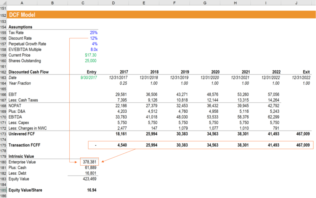
We all deal with numbers in one way or the other. We all have daily expenses which we pay for from the monthly income that we earn. For one to spend wisely, they will need to know their income vs. expenditure. Microsoft Excel comes in handy when we want to record, analyze and store such numeric data. Let’s illustrate this using the following image.

Where can I get Microsoft Excel?
There are number of ways in which you can get Microsoft Excel. You can buy it from a hardware computer shop that also sells software. Microsoft Excel is part of the Microsoft Office suite of programs. Alternatively, you can download it from the Microsoft website but you will have to buy the license key.
In this Microsoft Excel tutorial, we are going to cover the following topics about MS Excel.
- How to Open Microsoft Excel?
- Understanding the Ribbon
- Understanding the worksheet
- Customization Microsoft Excel Environment
- Important Excel shortcuts
How to Open Microsoft Excel?
Running Excel is not different from running any other Windows program. If you are running Windows with a GUI like (Windows XP, Vista, and 7) follow the following steps.
- Click on start menu
- Point to all programs
- Point to Microsoft Excel
- Click on Microsoft Excel
Alternatively, you can also open it from the start menu if it has been added there. You can also open it from the desktop shortcut if you have created one.
For this tutorial, we will be working with Windows 8.1 and Microsoft Excel 2013. Follow the following steps to run Excel on Windows 8.1
- Click on start menu
- Search for Excel N.B. even before you even typing, all programs starting with what you have typed will be listed.
- Click on Microsoft Excel
The following image shows you how to do this

Understanding the Ribbon
The ribbon provides shortcuts to commands in Excel. A command is an action that the user performs. An example of a command is creating a new document, printing a documenting, etc. The image below shows the ribbon used in Excel 2013.

Ribbon components explained
Ribbon start button – it is used to access commands i.e. creating new documents, saving existing work, printing, accessing the options for customizing Excel, etc.
Ribbon tabs – the tabs are used to group similar commands together. The home tab is used for basic commands such as formatting the data to make it more presentable, sorting and finding specific data within the spreadsheet.
Ribbon bar – the bars are used to group similar commands together. As an example, the Alignment ribbon bar is used to group all the commands that are used to align data together.
Understanding the worksheet (Rows and Columns, Sheets, Workbooks)
A worksheet is a collection of rows and columns. When a row and a column meet, they form a cell. Cells are used to record data. Each cell is uniquely identified using a cell address. Columns are usually labelled with letters while rows are usually numbers.
A workbook is a collection of worksheets. By default, a workbook has three cells in Excel. You can delete or add more sheets to suit your requirements. By default, the sheets are named Sheet1, Sheet2 and so on and so forth. You can rename the sheet names to more meaningful names i.e. Daily Expenses, Monthly Budget, etc.

Customization Microsoft Excel Environment
Personally I like the black colour, so my excel theme looks blackish. Your favourite colour could be blue, and you too can make your theme colour look blue-like. If you are not a programmer, you may not want to include ribbon tabs i.e. developer. All this is made possible via customizations. In this sub-section, we are going to look at;
- Customization the ribbon
- Setting the colour theme
- Settings for formulas
- Proofing settings
- Save settings
Customization of ribbon

The above image shows the default ribbon in Excel 2013. Let’s start with customization the ribbon, suppose you do not wish to see some of the tabs on the ribbon, or you would like to add some tabs that are missing such as the developer tab. You can use the options window to achieve this.
- Click on the ribbon start button
- Select options from the drop down menu. You should be able to see an Excel Options dialog window
- Select the customize ribbon option from the left-hand side panel as shown below

- On your right-hand side, remove the check marks from the tabs that you do not wish to see on the ribbon. For this example, we have removed Page Layout, Review, and View tab.
- Click on the “OK” button when you are done.
Your ribbon will look as follows

Adding custom tabs to the ribbon
You can also add your own tab, give it a custom name and assign commands to it. Let’s add a tab to the ribbon with the text Guru99

- Right click on the ribbon and select Customize the Ribbon. The dialogue window shown above will appear
- Click on new tab button as illustrated in the animated image below
- Select the newly created tab
- Click on Rename button
- Give it a name of Guru99
- Select the New Group (Custom) under Guru99 tab as shown in the image below
- Click on Rename button and give it a name of My Commands
- Let’s now add commands to my ribbon bar
- The commands are listed on the middle panel
- Select All chart types command and click on Add button
- Click on OK
Your ribbon will look as follows

Setting the colour theme
To set the color-theme for your Excel sheet you have to go to Excel ribbon, and click on à File àOption command. It will open a window where you have to follow the following steps.

- The general tab on the left-hand panel will be selected by default.
- Look for colour scheme under General options for working with Excel
- Click on the colour scheme drop-down list and select the desired colour
- Click on OK button
Settings for formulas
This option allows you to define how Excel behaves when you are working with formulas. You can use it to set options i.e. autocomplete when entering formulas, change the cell referencing style and use numbers for both columns and rows and other options.

If you want to activate an option, click on its check box. If you want to deactivate an option, remove the mark from the checkbox. You can this option from the Options dialogue window under formulas tab from the left-hand side panel
Proofing settings

This option manipulates the entered text entered into excel. It allows setting options such as the dictionary language that should be used when checking for wrong spellings, suggestions from the dictionary, etc. You can this option from the options dialogue window under the proofing tab from the left-hand side panel
Save settings

This option allows you to define the default file format when saving files, enable auto recovery in case your computer goes off before you could save your work, etc. You can use this option from the Options dialogue window under save tab from the left-hand side panel
Important Excel shortcuts
| Ctrl + P | used to open the print dialogue window |
| Ctrl + N | creates a new workbook |
| Ctrl + S | saves the current workbook |
| Ctrl + C | copy contents of current select |
| Ctrl + V | paste data from the clipboard |
| SHIFT + F3 | displays the function insert dialog window |
| SHIFT + F11 | Creates a new worksheet |
| F2 | Check formula and cell range covered |
Best Practices when working with Microsoft Excel
- Save workbooks with backward compatibility in mind. If you are not using the latest features in higher versions of Excel, you should save your files in 2003 *.xls format for backwards compatibility
- Use description names for columns and worksheets in a workbook
- Avoid working with complex formulas with many variables. Try to break them down into small managed results that you can use to build on
- Use built-in functions whenever you can instead of writing your own formulas
Summary
- Introduction of MS Excel : Microsoft Excel is a powerful spreadsheet program used to record, manipulate, store numeric data and it can be customized to match your preferences
- The ribbon is used to access various commands in Excel
- The options dialogue window allows you to customize a number of items i.e. the ribbon, formulas, proofing, save, etc.