
Содержание
- VBA Dynamic Range
- Referencing Ranges and Cells
- Range Property
- Cells Property
- Dynamic Ranges with Variables
- Last Row in Column
- Last Column in Row
- VBA Coding Made Easy
- SpecialCells – LastCell
- UsedRange
- CurrentRegion
- Named Range
- Tables
- VBA Code Examples Add-in
- Introduction to Dynamic Ranges
- How to create and use dynamic named range in Excel
- How to create a dynamic named range in Excel
- OFFSET formula to define an Excel dynamic named range
- INDEX formula to make a dynamic named range in Excel
- How to make two-dimensional dynamic range in Excel
- How to use dynamic named ranges in Excel formulas
- You may also be interested in
VBA Dynamic Range
In this Article
This article will demonstrate how to create a Dynamic Range in Excel VBA.
Declaring a specific range of cells as a variable in Excel VBA limits us to working only with those particular cells. By declaring Dynamic Ranges in Excel, we gain far more flexibility over our code and the functionality that it can perform.
Referencing Ranges and Cells
When we reference the Range or Cell object in Excel, we normally refer to them by hardcoding in the row and columns that we require.
Range Property
Using the Range Property, in the example lines of code below, we can perform actions on this range such as changing the color of the cells, or making the cells bold.
Cells Property
Similarly, we can use the Cells Property to refer to a range of cells by directly referencing the row and column in the cells property. The row has to always be a number but the column can be a number or can a letter enclosed in quotation marks.
For example, the cell address A1 can be referenced as:
To use the Cells Property to reference a range of cells, we need to indicate the start of the range and the end of the range.
For example to reference range A1: A6 we could use this syntax below:
We can then use the Cells property to perform actions on the range as per the example lines of code below:
Dynamic Ranges with Variables
As the size of our data changes in Excel (i.e. we use more rows and columns that the ranges that we have coded), it would be useful if the ranges that we refer to in our code were also to change. Using the Range object above we can create variables to store the maximum row and column numbers of the area of the Excel worksheet that we are using, and use these variables to dynamically adjust the Range object while the code is running.
Last Row in Column
As there are 1048576 rows in a worksheet, the variable lRow will go to the bottom of the sheet and then use the special combination of the End key plus the Up Arrow key to go to the last row used in the worksheet – this will give us the number of the row that we need in our range.
Last Column in Row
Similarly, the lCol will move to Column XFD which is the last column in a worksheet, and then use the special key combination of the End key plus the Left Arrow key to go to the last column used in the worksheet – this will give us the number of the column that we need in our range.
Therefore, to get the entire range that is used in the worksheet, we can run the following code:
VBA Coding Made Easy
Stop searching for VBA code online. Learn more about AutoMacro — A VBA Code Builder that allows beginners to code procedures from scratch with minimal coding knowledge and with many time-saving features for all users!

SpecialCells – LastCell
We can also use SpecialCells method of the Range Object to get the last row and column used in a Worksheet.
UsedRange
The Used Range Method includes all the cells that have values in them in the current worksheet.
CurrentRegion
The current region differs from the UsedRange in that it looks at the cells surrounding a cell that we have declared as a starting range (ie the variable rngBegin in the example below), and then looks at all the cells that are ‘attached’ or associated to that declared cell. Should a blank cell in a row or column occur, then the CurrentRegion will stop looking for any further cells.
If we use this method, we need to make sure that all the cells in the range that you require are connected with no blank rows or columns amongst them.
Named Range
We can also reference Named Ranges in our code. Named Ranges can be dynamic in so far as when data is updated or inserted, the Range Name can change to include the new data.
This example will change the font to bold for the range name “January”
As you will see in the picture below, if a row is added into the range name, then the range name automatically updates to include that row.
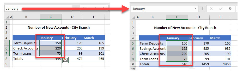
Should we then run the example code again, the range affected by the code would be C5:C9 whereas in the first instance it would have been C5:C8.
Tables
We can reference tables (click for more information about creating and manipulating tables in VBA) in our code. As a table data in Excel is updated or changed, the code that refers to the table will then refer to the updated table data. This is particularly useful when referring to Pivot tables that are connected to an external data source.
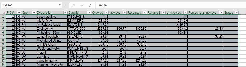
Using this table in our code, we can refer to the columns of the table by the headings in each column, and perform actions on the column according to their name. As the rows in the table increase or decrease according to the data, the table range will adjust accordingly and our code will still work for the entire column in the table.

VBA Code Examples Add-in
Easily access all of the code examples found on our site.
Simply navigate to the menu, click, and the code will be inserted directly into your module. .xlam add-in.
Источник
Introduction to Dynamic Ranges
An introduction to Dynamic Ranges
The VLOOKUP function is often used to find information that is stored within tables in Excel. So for example if we have a list of people’s names and ages:
And then we can in a nearby cell use the function VLOOKUP to determine Paul’s age:
So far this is a fairly standard. But what happens if we need to add some more names to the list ? The obvious thought would be to modify the range in the VLOOKUP. However, in a really complex model, there may be several references to the VLOOKUP. This means that we would have to change each reference – assuming that we knew where they were.
However Excel provides an alternative way – called a DYNAMIC range. This is a range that expands an updates automatically. This is perfect if your lists are for ever expanding (e.g month on month sales data).
To set up a dynamic range we need to have a range name – so we’ll call ours AGE_DATA. The approach for setting up dynamic ranges differs between Excel 2007 and earlier versions of Excel:
In Excel 2007, click on “Define Name” under formulae:
In earlier versions of Excel click on “Insert” and then Names” .
In the pop up box, enter the name of our dynamic range – which is “AGE DATA”:
In the box labeled “Refers To” we need to enter the range of our data. This is will be an achieved used by an OFFSET function. This has 5 arguments:
=OFFSET(Reference, Rows, Cols, Height, Width)
– The Reference is the address of the TOP LEFT corner of our range – in this case cell B5
– The Rows is the number of rows from the TOP LEFT that we want that range to be – which will be 0 in this case
– The Cols is the number of rows from the TOP LEFT that we want that range to be – which will be 0 in this case
– The Height of the range – see below for this
– The Width of the range – this is 2 has we have TWO columns in our range (the persons name and their age)
Now the height of the range will have to vary depending on the number of entries in our table (which is currently 7).
Of course we want a way of counting up the rows in our table that updates automatically – so one way of doing this is to use the COUNTA function. This just counts up the number of non blank cells in a range. As our names are in column B, the number of entries in our data is COUNTA(B:B).
Note that if you were to put this in a cell you would get the value 8 – as it includes the header Names. However, that it is immaterial.
So in the “Refers To” box we put:
And click the OK button. Our dynamic range is now created.
Now return to the VLOOKUP formulae and replace the range $B:4:$C11 with the name of our new dynamic range AGE_DATA so we have:
So far nothing has changed. However if we add a few more names to our table:
And in the cell where we had Paul, replace it with a new name such as Pedro (that wasn’t on original list):
And we see that Excel has automatically returned Pedro’s age – even though we haven’t changed the VLOOKUP formulae. Instead the scope of the dynamic range has increased to include the extra names.
Dynamic ranges are very useful when we have increasing volumes of data – especially when VLOOKUP and PIVOT tables are required.
Источник
How to create and use dynamic named range in Excel
 by Svetlana Cheusheva, updated on March 1, 2023
In this tutorial, you will learn how to create a dynamic named range in Excel and how to use it in formulas to have new data included in calculations automatically.
In last week’s tutorial, we looked at different ways to define a static named range in Excel. A static name always refers to the same cells, meaning you would have to update the range reference manually whenever you add new or remove existing data.
If you are working with a continuously changing data set, you may want to make your named range dynamic so that it automatically expands to accommodate newly added entries or contracts to exclude removed data. Further on in this tutorial, you will find detailed step-by-step guidance on how to do this.
How to create a dynamic named range in Excel
For starters, let’s build a dynamic named range consisting of a single column and a variable number of rows. To have it done, perform these steps:
- On the Formula tab, in the Defined Names group, click Define Name. Or, press Ctrl + F3 to open the Excel Name Manger, and click the New… button.
- Either way, the New Name dialogue box will open, where you specify the following details:
- In the Name box, type the name for your dynamic range.
- In the Scope dropdown, set the name’s scope. Workbook (default) is recommended in most cases.
- In the Refers to box, enter either OFFSET COUNTA or INDEX COUNTA formula.
- Click OK. Done!
In the following screenshot, we define a dynamic named range items that accommodates all cells with data in column A, except for the header row: 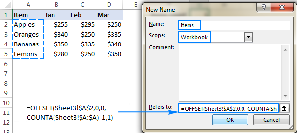
OFFSET formula to define an Excel dynamic named range
The generic formula to make a dynamic named range in Excel is as follows:
- first_cell — the first item to be included in the named range, for example $A$2.
- column — an absolute reference to the column like $A:$A.
At the core of this formula, you use the COUNTA function to get the number of non-blank cells in the column of interest. That number goes directly to the height argument of the OFFSET(reference, rows, cols, [height], [width]) function telling it how many rows to return.
Beyond that, it’s an ordinary Offset formula, where:
- reference is the starting point from which you base the offset (first_cell).
- rows and cols are both 0, since there are no columns or rows to offset.
- width is equal to 1 column.
For example, to build a dynamic named range for column A in Sheet3, beginning in cell A2, we use this formula:
=OFFSET(Sheet3!$A$2, 0, 0, COUNTA(Sheet3!$A:$A), 1)
Note. If you are defining a dynamic range in the current worksheet, you do not need to include the sheet name in the references, Excel will do it for you automatically. If you are building a range for some other sheet, prefix the cell or range reference with the sheet’s name followed by the exclamation point (like in the formula example above).
INDEX formula to make a dynamic named range in Excel
Another way to create an Excel dynamic range is using COUNTA in combination with the INDEX function.
This formula consists of two parts:
- On the left side of the range operator (:), you put the hard-coded starting reference like $A$2.
- On the right side, you use the INDEX(array, row_num, [column_num]) function to figure out the ending reference. Here, you supply the entire column A for the array and use COUNTA to get the row number (i.e. the number of non-entry cells in column A).
For our sample dataset (please see the screenshot above), the formula goes as follows:
Since there are 5 non-blank cells in column A, including a column header, COUNTA returns 5. Consequently, INDEX returns $A$5, which is the last used cell in column A (usually an Index formula returns a value, but the reference operator forces it to return a reference). And because we have set $A$2 as the starting point, the final result of the formula is the range $A$2:$A$5.
To test the newly created dynamic range, you can have COUNTA fetch the items count:
=COUNTA(Items) 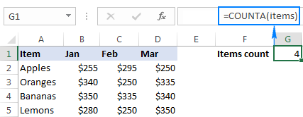
If all done properly, the result of the formula will change once you add or remove items to/from the list: 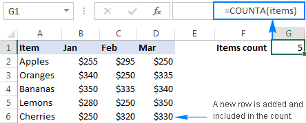
Note. The two formulas discussed above produce the same result, however there is a difference in performance you should be aware of. OFFSET is a volatile function that recalculates with every change to a sheet. On powerful modern machines and reasonably sized data sets, this should not be a problem. On low-capacity machines and large data sets, this may slow down your Excel. In that case, you’d better use the INDEX formula to create a dynamic named range.
How to make two-dimensional dynamic range in Excel
To build a two-dimensional named range, where not only the number of rows but also the number of columns is dynamic, use the following modification of the INDEX COUNTA formula:
In this formula, you have two COUNTA functions to get the last non-empty row and last non-empty column (row_num and column_num arguments of the INDEX function, respectively). In the array argument, you feed the entire worksheet (1048576 rows in Excel 2016 — 2007; 65535 rows in Excel 2003 and lower).
And now, let’s define one more dynamic range for our data set: the range named sales that includes sales figures for 3 months (Jan to Mar) and adjusts automatically as you add new items (rows) or months (columns) to the table.
With the sales data beginning in column B, row 2, the formula takes the following shape:
=$B$2:INDEX($1:$1048576,COUNTA($B:$B),COUNTA($2:$2)) 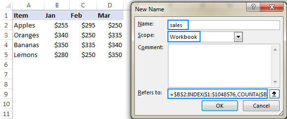
To make sure your dynamic range works as it is supposed to, enter the following formulas somewhere on the sheet:
As you can see in the screenshot bellow, both formulas return the same total. The difference reveals itself in the moment you add new entries to the table: the first formula (with the dynamic named range) will update automatically, whereas the second one will have to be updated manually with each change. That makes a huge difference, uh? 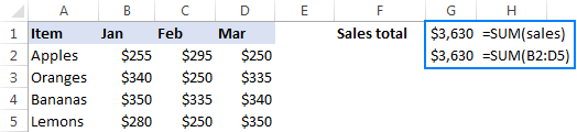
How to use dynamic named ranges in Excel formulas
In the previous sections of this tutorial, you have already seen a couple of simple formulas that use dynamic ranges. Now, let’s try to come up with something more meaningful that shows the real value of an Excel dynamic named range.
For this example, we are going to take the classic INDEX MATCH formula that performs Vlookup in Excel:
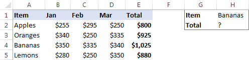
…and see how we can make the formula even more powerful with the use of dynamic named ranges.
As shown in the screenshot above, we are attempting to build a dashboard, where the user enters an item name in H1 and gets the total sales for that item in H2. Our sample table created for demonstration purposes contains only 4 items, but in your real-life sheets there can be hundreds and even thousands of rows. Furthermore, new items can be added on a daily basis, so using references is not an option, because you’d have to update the formula over and over again. I’m too lazy for that! 🙂
To force the formula to expand automatically, we are going to define 3 names: 2 dynamic ranges, and 1 static named cell:
Lookup_range: =$A$2:INDEX($A:$A, COUNTA($A:$A))
Return_range: =$E$2:INDEX($E:$E, COUNTA($E:$E))
Note. Excel will add the name of the current sheet to all references, so before creating the names be sure to open the sheet with your source data.
Now, start typing the formula in H1. When it comes to the first argument, type a few characters of the name you want to use, and Excel will show all available matching names. Double-click the appropriate name, and Excel will insert it in the formula right away: 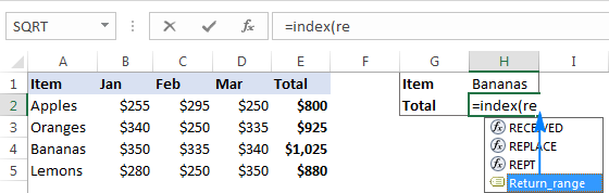
The completed formula looks as follows:
=INDEX(Return_range, MATCH(Lookup_value, Lookup_range, 0))
And works perfectly! 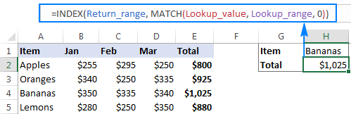
As soon as you add new records to the table, they will be included in your calculations at once, without you having to make a single change to the formula! And if you ever need to port the formula to another Excel file, simply create the same names in the destination workbook, copy/paste the formula, and get it working immediately.
Tip. Apart from making formulas more durable, dynamic ranges come in handy for creating dynamic dropdown lists.
This is how you create and use dynamic named ranges in Excel. To have a closer look the formulas discussed in this tutorial, you are welcome to download our sample Excel Dynamic Named Range Workbook. I thank you for reading and hope to see you on our blog next week!
You may also be interested in
Table of contents
I have production report with two columns one column for dates and second column is for case number so I need result how many case number completes for the date.
Example.
A column B column
03/13/23 AS123
03/13/23 AS234
03/14/23 AS768
I need countifs formula for with match date on second sheet.
Hi!
For the answer to your question and examples of formulas, see here: Using Excel COUNTIF function with dates.
Image attached is the best way to understand what the formula supposed to achieve and the problem I am trying to resolve. However, I will try to explain the requirement which the calculation is trying to satisfy.
Business Entity (Corporation, such as Amazon) — US Tax Code allow a business to carryforward Operating Loss of a business entity to be used to OFFSET income in future years, until the loss is fully used. Depending on the income in future years, previous year(s) loss can be completely utilized in «One Single Year», or spread across multiple years (as shown in Row 33 — Year = 2017)
As shown in the table below, the first three columns capture the details such as NOL Generated Amount, Used, or Expired for the Year of NOL Generated which is mentioned in column «Year». Column H calculate how much of the income from the Year (mentioned in Year column) is used in «Current Year» (which in this example is 2022 — bottom row).
Now, based on the above-mentioned facts so far, the calculation is straightforward, where Total Available column give me the amount of NOL that can be used for Current Year, and the amount utilized needs to be deducted from the Income as calculation progress through subsequent years.
**
Here comes the Wrinkle and hence my problem, because of Tax Rule Changes:
Post 2017, there is difference between how the NOL is treated (or for that matter, how much of it can be used). NOLs generated prior to 2018 (Year Reply
Hi!
Try creating a dynamic reference using the INDIRECT function.
You can find the examples and detailed instructions here: Excel INDIRECT function — basic uses and formula examples. I hope it’ll be helpful.
Good day, I need some assistance please. I have an excel sheet with Dynamic columns. I display the total Working hours in columnD and only display the overtime hours if there are any. If there isn’t any overtime hours then I display the week in days starting from either column E or columnG. I need to sort the days of the week according to a date range which I have just specified. So, If my Monday falls on the 19th and my Thursday falls on the 13th, I need to sort the columns so that Thursday comes first and Wednesday comes last. I don’t know the column letter (could be D or E or F or G or so on) but I can determine the letter. I don’t want to use the letter but when I substitute, I get an error. When I run the hardcoded substitution, it works fine «Sheets(sheetName).Range(«I2:O132»).Sort Key1:=Range(«I2:O2″), Order1:=xlAscending, Orientation:=xlLeftToRight». When I use the following, I get an error Sheets(sheetName).Range((«»»» & strColumnStart & «» & «:» & «» & strColumnEnd & «»»»)).Sort Key1:=Range(«»»» & strColumnStart & «» & «:» & «» & strColumn & «»»»), Order1:=xlAscending, Orientation:=xlLeftToRight. When I use the immediate window, «»»» & strColumnStart & «» & «:» & «» & strColumnEnd & «»»» equates to «I2:O132» but it just doesn’t work. Does anyone have a solution to this?
Hi!
Unfortunately, we can only help with writing Excel formulas. Your problem cannot be solved with formulas.
How to Create a name manager if the is many blank cells in between cells
=SUMPRODUCT(((Airport!$B$5:$B$2000)=$A$6)*((Airport!$C$5:$C$2000)=C2),(Airport!D5:D2000)) works perfect so added your formula to create a dynamic range.
=SUMPRODUCT(((Mon_Col2)=$A$6)*((Airport!$C$5:$C$2000)=C2),(Airport!D5:D2000)) when you step in and evaluate the formula it does return the correct dynamic range. However it gives me a #N/A error when finished.
Hello!
I can’t see your data, but I can assume that your dynamic ranges are different sizes.
HI,
I have created a table using dynamic range. I would like to format(meaning color/borders) like a when I create a table with alternating fill colors for row. Is there a simple method?
The button Labeled «Format as Table» creates a table them my Dynamic range goes to Spill Error.
Hello!
You cannot create an Excel table from a named range. You need to convert formulas to values. Or use standard Excel formatting tools.
Here is the article that may be helpful to you: Highlight every other row in Excel using conditional formatting.
Here’s a weird one for dynamic range defined in Formulas>Name Manager (Excel MAc v16.59).
Trying to define/name a dynamic range $L$1:$M$M from Parameters! Tab using:
=OFFSET(Parameters!$L$1,0,0,COUNTA(Parameters!$M:$M),2)
1) Type that into any cell in the workbook (even other Tabs) and seems to return exactly whats desired.
2) Type that into the Name Manager to assign a name to this dynamic range and get nothing returned. no error message, just an empty set of data.
Any ideas or possibly is there a bug in the Excel Mac?
Thanks for any response.
Hello!
Unfortunately, I was unable to reproduce your situation on Excel for Mac. I pasted your formula into the «Refers to» field and got a working named range.
Check if you are doing everything correctly in accordance with the instructions described in the article above.
I’m having trouble entering the formula for a dynamic range.
=Sheet1!ADDRESS(MATCH(TODAY():$P:$P,0),16):INDEX($P:$P, COUNTA($P:$P))
or
=Sheet1!ADDRESS(MATCH(TODAY(),P10:P374,0),16):$P$374
Keeps giving me a message about am I trying to enter a formula, must start with= or -.
When I enter only the cell formula, it takes it, but I need a range.
=Sheet1!ADDRESS(MATCH(TODAY():$P:$P,0),16) Works to give the cell address of today’s date.
This creates dynamic range starting at today’s date in column P and I want to extend it to the end of the data in column P. Column P is a list of dates.
I need this to then find the next value in a different column after the today’s date row.
This different than most dynamic ranges that only extend the bottom. I want to do both. One to move the top based on today’s date and the bottom to extend it based on data being added.
I hope you can help me. I’ve learned a lot from you.
Thanks,
Colt
Hello!
If your list of dates starts in cell A1, then you can use the formula to create a dynamic range starting from the current date:
This should solve your task.
Hi,
How can I get the Defined Name to work for a dynamic range when I have both Blank and Non-Blank cells within my range?
Hello!
Try using the COUNTBLANK function in your dynamic range formula:
OFFSET(first_cell, 0, 0, COUNTA(column)+COUNTBLANK(column), 1)
I hope it’ll be helpful.
I don’t think this will work. The COUNTBLANK function will also count all of the blanks below the last item in the column giving you a very large value for modern versions of Excel.
Hi!
Of course, you can use a range of cells instead of the entire column in the formula.
For example — Instead of COUNTA(column) use COUNTA(A1:A100)
This will seriously speed up the calculations.
Each day I copy a watchlist of share prices from Yahoo Finance to Excel. By placing the latest end-of day closing share prices in the right-most column of a table, all the previous entries move one column to the left. (Excel does that for me).
Every day’s close-price of each company, from start date to the present, is listed in a row. The column holding the start date, is moving leftwards into another column, day by day.
I make charts of each company. The chart includes the Start date, (when I first started taking the company’s data). The chart records up to the present day.
I know where is each start date. By using Index and Match I can find exactly in which column is the Start date. I can list the column reference in a cell:- e.g in cell Q1 is listed, column «CME».
Today, the column holding my start date for the company, RCP.L, is CME. Yesterday, before I took the day’s figures, it was CMF.
I now want an automatic facility (formula) to enter CME14:CME770 into an INDEX & MATCH formula (below) which, yesterday was reading CMF14:CMF770:-
So the Index Match formula for yesterday is:-
INDEX(Close!CMF$14:CMF$770,MATCH($Q$1,Close!$ATK$14:$ATK$770,0))
It reads yesterday’s range, not today’s.
($SQ$S1 reads the cell containing «RCP.L» to find the row in the column range CMF14:CMF770.)
Today I want the INDEX Match formula to be
INDEX(Close!CME$14:CME$770,MATCH($Q$1,Close!$ATK$14:$ATK$770,0))
Tomorrow I will want CMD14:CMD770 in the formula and so-on.
I’ve done masses of reading and completely stuck. Can you please help? Regards, Philip.
Hello!
How do I create a Dynamic Named Range for unlocked ranges by a password when sheet is protected.
How do I create a Dynamic Named Range for unlocked range by a password?
I would like to add numbers in a column
using sum, offset, counta and the column has a name.
For practice, I have column E and beginning with row 3 the title: salary. Rows 4, 5, 6,etc are the salaries. Column E3:E10 has been named as «monthly_salaries». I need to use that so I can place the sum(monthly_salaries) function on any worksheet, while the monthly-salaries will be on a seperate worksheet.
Each month the length of this vertical column E changes as more or less people draw salaries. Also, I use different worksheets so data, like the salaries may be located on worksheet 2 and the actual sum on worksheet 1.
I have offset(e3,0,0,counta(E:E),1.
Question: How to combine the column name with the sum function to accommodate the dynamic nature of this problem.
Thank you for your assistance.
Chris
Hello!
Create a dynamic named range “monthly_salaries” using a formula
=OFFSET($E$3, 0, 0, COUNTA($E$3:$E$10), 1)
Use it like this:
I hope I answered your question.
Dynamic Named Ranges don’t seem to like Dynamic Array Formulas it seems.
I have 2 Dynamic Named Ranges, say LIST1 and LIST2. In a separate column, I have entered the formula: FILTER(LIST1, LIST2=»an existing value»). This returns an error (#VALUE!). It worked correctly when my named ranges were not dynamic.
Is there an evident reason why I am getting this error?
Thanks in advance!
Sabrina
Hello!
I was unable to repeat your errors. I don’t have your data.
Please have a look at this article — FILTER function not working.
I hope my advice will help you solve your task.
Hi, How do i use Dynamic Named Range in «Data Rane» Excel chart ?
=$B$2:INDEX($1:$1048576,COUNTA($B:$B),COUNTA($2:$2)) or =$A$2:INDEX($A:$A, COUNTA($A:$A))
is not suitable for this.
Thank You,
Ofer
hi there.. hope someone could help me. I want to create a name in my file which is getting values from a single column table. I want to exclude one specific value and don’t want it to be part of the name range. Not sure how can I do that? Column data is:
Fruits (table header)
Apple
Banana
Orange
Grapes
Want to have a list that exclude «Orange». As it’s a table I will be adding new names after Grapes in near future.
Hello, I am painfully new to working with Excel, macros, and the like. I have recorded a macro, but right now it will only work on the cell range that I originally recorded the macro on. Right now the range reads as =Range(«A2:A724»), but I need the bottom part of the range (A724) to be dependent on column B. Meaning, if column B has data going down to cell B1021, then I want my range in column A to automatically look like =Range(«A2:A1021»). I would appreciate any help. Thanks!
Hi! I’m a newbie in Excel, so there’s a risk my question is kind os obvious. I’m trying to connect a Pivot Table in Excel to a Word File, for this, I have to edit the Name of my range in Excel and Word so the Word table automatically updates the range it is reporting. The problem I have is Excel says he doesn’t understand my formula, it looks like this:
Where DE40 is the Sheet/Pivot Table I’m trying to refer. Any ideas?
I have a simple table: 7 columns, 4 rows. Can I create a formula just adding Hrs of bananas?
Jan 1 Jan 2 Jan 3
Hrs Cases Hrs Cases Hrs Cases
Bananas 1 10 3 30 0 0
Apples 5 20 1 4 3 12
_______|___Hrs_|_Cases_|_Hrs_|_Cases_|_Hrs_|_Cases
Bananas|____1__|___10__|__3__|___30___|_0__|___0__
Apples_|____5__|___20__|__1__|___04___|_3__|___12_
No sure if this will help to understand the table.
An easy way to do it if you need a range is to use indirect in the name.. eg example for A2:G10
There is 20 rows in coloumn A
since indirect «translate» the expression — so it reads the name to be refered to this
Sheet_name!A2:G10
Correction — There is 20 rows in coloumn A — should ofcourse be 10 rows 😉
I’m trying to create a dynamic range showing client names only if their status is Active in another column. Can someone help me with the formula for this?
This index formula method for creating dynamic named range is not working.
Using evaluate formula, this shows to result to $H$2:$H$6. But post that it acts as an array formula. Its finally returning value either H2/H3/H4/H5/H6 based on the cell.
What i mean to say is, it is not giving a range. Hence, this seems wrong.
Please let me know your view.
Hi
How do you create a Dynamic named range (with INDEX) but without the sheet name automatically added after the Define Name editor is closed?
Tnks
THANK YOU FOR ENLIGHTENING ME
AM SO DAMN GRATEFUL FOR THIS WRITE UP
How do I create a Dynamic Named Range with worksheets instead of rows or columns?
I have a workbook that I add a new worksheet to every week and I want to track my vacation time over the course of the calendar year.
Thank you for your help.
Copyright © 2003 – 2023 Office Data Apps sp. z o.o. All rights reserved.
Microsoft and the Office logos are trademarks or registered trademarks of Microsoft Corporation. Google Chrome is a trademark of Google LLC.
Источник
Excel Dynamic Range (Table of Contents)
- Dynamic Range in Excel
- Uses of Dynamic Range
- How to Create a Dynamic Range in Excel?
Dynamic Range in Excel
Dynamic Range in excel allows us to use the newly updated range always whenever the new set of lines are appended in the data. It just gets updated automatically when we add new cells or rows. We have used a static range where value cells are fixed, and herewith a Dynamic range, our range will change as well add the data. This can be done in any function in excel. And for this, we have an option in excel available in the Formula tab under defined names as Name Manager.
Below are the examples for range:
Uses of Dynamic Range
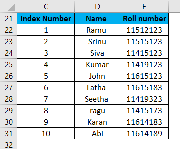
Let’s assume you have to give an index number for a database range of 100 rows. As we have 100 rows, we need to give 100 index numbers vertically from top to bottom. Suppose we type that 100 numbers manually; it will take around 5-10 minutes of time. Here range helps to make this task within 5 seconds of time. Let’s see how it will work.
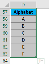
We need to achieve the index numbers as shown in the below screenshot; here, I give an example only for 10 rows.
Give the first two numbers under the index number, select the range of two numbers as shown below, and click on the corner (Marked in red colour).
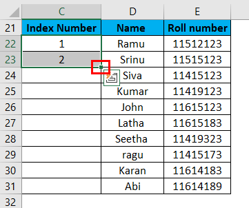
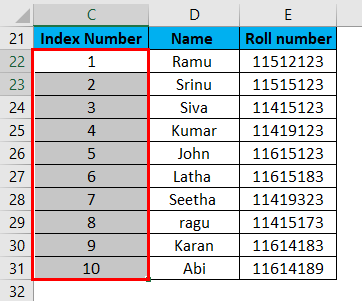
Drag until the required range. It will give the continuous series as per the first two numbers pattern.
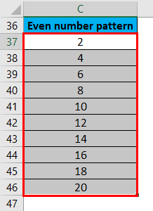
If we give the first cell as 2 and the second cell as 4, then it will give all the even numbers. Select the range of two numbers as shown below and click on the corner (Marked in red colour).
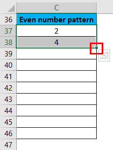
Drag until the required range. It will give the continuous series as per the first two numbers pattern.
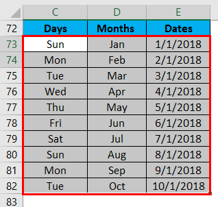
The same will apply for months, days, dates etc.…Provide the first two values of the required pattern, highlight the range, and then click on the corner.
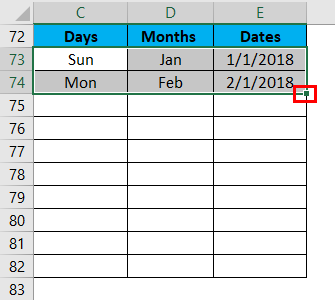
Drag until the required length. It will give the continuous series as per the first two numbers pattern.
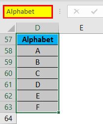
I hope you understand what it is a range; now, we will discuss the dynamic range. You can give a name to a range of cells by simply selecting the range.
Give the name in the name box (highlighted in the screenshot).
Please select the Name which we added and press enter.
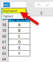
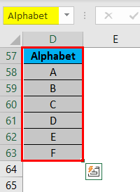
So that when you select that name, the range will pick automatically.
Dynamic Range in Excel
Dynamic range is nothing but the range that picked dynamically when additional data is added to the existing range.
Example
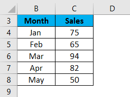
See the below sales chart of a company from Jan to Apr.
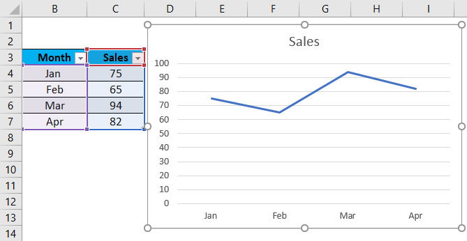
When we update May below the Apr month data’s sales in May month, the sales chart will update automatically (Dynamically). This is happening because the range we used is dynamic range; hence, the chart takes the dynamic range and changes the chart accordingly.

If the range is not a dynamical range, then the chart will not automatically update when we update the data to the existing data range.
We can achieve the Dynamic range in two ways.
- Using Excel table feature
- Using Offsetting entry
How to Create a Dynamic Range in Excel?
Dynamic range in Excel is straightforward and easy to correct. Let’s understand how to Create a Dynamic range with some Examples.
You can download this Dynamic Range Excel Template here – Dynamic Range Excel Template
Dynamic Range in Excel Example #1 – Excel Table feature
We can achieve the Dynamic range by using this feature, but this will apply if we use the excel version of 2017 and the versions released after 2017.
Let’s see how to create now. Take a database range like below.
Select the entire data range and click on the insert button at the top menu bar marked in red colour.
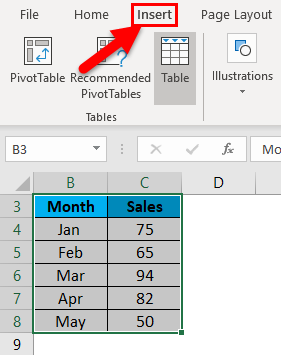
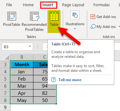
Later click on the table below the insert menu.
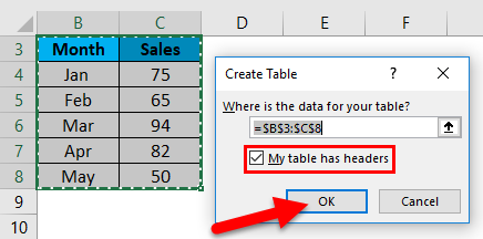
The below-shown pop up will come; check the field ‘My table has header’ as our selected data table range has a header and Click ‘Ok’.
Then the data format will change to table format; you can observe the colour also.

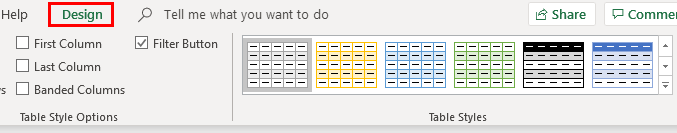
If you want to change the format(colour), select the table and click on the top menu bar’s design button. You can select the required formats from the ‘table styles’.
Now the data range is in table format; hence whenever you add new data lines, the table feature makes the data range update dynamically into a table; hence the chart also changes dynamically. Below is the screenshot for reference.
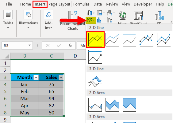
Click on insert and go to charts and Click on Line chart as shown below.
A-Line Chart is added, as shown below.
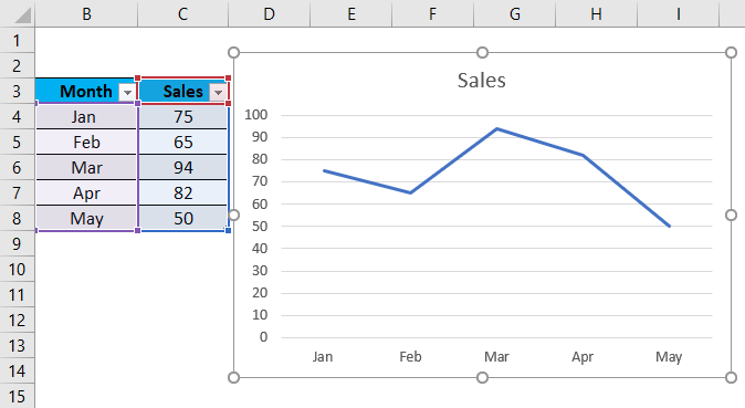
If you add one more data to the table, i.e. Jun and sales as 100, then the chart is automatically updated.

This is one way of creating a dynamical data range.
Dynamic Range in Excel Example #2 – Using the offsetting entry
The offsetting formula helps to start with a reference point and can offset down with the required number of rows and right or left with required numbers of columns into our table range.
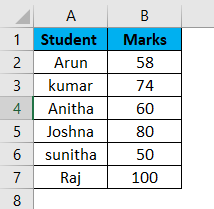
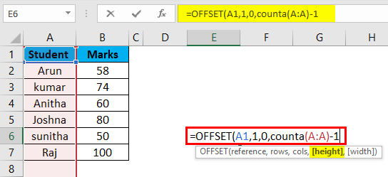
Let’s see how to achieve dynamic range using the offsetting formula. Below is the data sample of the student table for creating a dynamic range.
To explain to you the format of offset, I am giving the formula in the normal sheet instead of applying it in the “Define name”.
Offset entry format
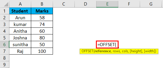
- Reference: Refers to the reference cell of the table range, which is the starting point.
- Rows: Refers to the required number of rows to offset below the starting reference point.
- Cols: Refers to the required number of columns to offset right or left to the starting point.
- Height: Refers to the height of the rows.
- Width: Refers to the Width of the columns.
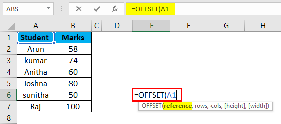
Start with the reference cell, where a student is the reference cell where you want to start a data range.
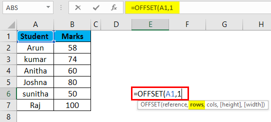
Now give the required number of rows to go down to consider into the range. Here ‘1’ is given because it is one row down from the reference cell.
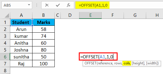
Now give the columns as 0 as we are not going to consider the columns here.
Now give the height of rows as we are not sure how many rows we will add in the future; hence, give the ‘counta’ function of rows (select the entire ‘A’ column). But we are not treating the header into range, so reduce by 1.
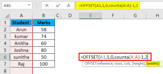
Now in Width, give 2 as here we have two columns, and we do not want to add any additional columns here. In case if we are not aware of how many columns we are going to add in future, then apply the ‘counta’ function to the entire row as how we applied to height. Close the formula.
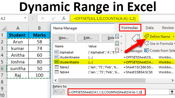
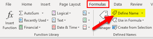
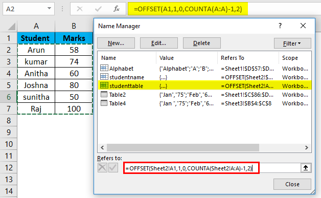
Now we need to apply the offset formula in the defined name to create a dynamic range. Click on the “formula” menu at the top (highlighted).
Click on the option “Define Name “ marked in the below screenshot.
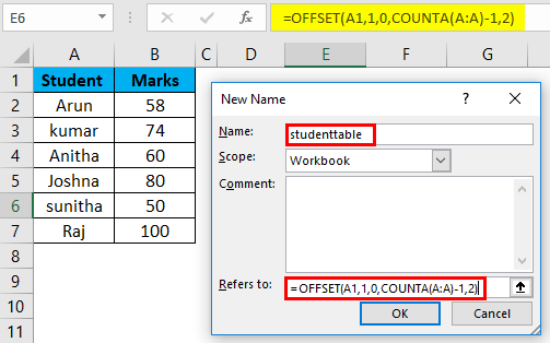
A popup will come, give the name of table range as ‘student table without space. ‘Scope’ leave it like a ‘Workbook’ and then go to ‘Refers to’ where we need to give the “OFFSET” formula. Copy the formula which we prepared priory and paste in Refers to
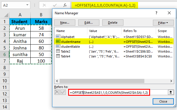
Now we can check the range by clicking on the Name manager and select the Name you provided in the Define name.
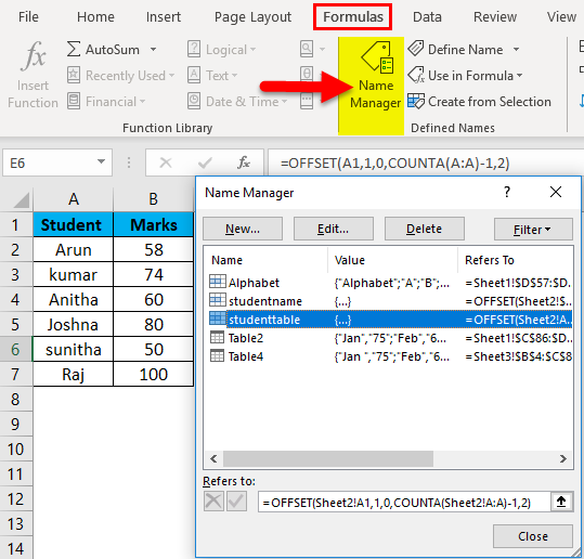
Here it is “Studenttable”, and then click on the formula to automatically highlight the table range, as you can observe in the screenshot.
If we add another line item to the existing range, the range will pick automatically. You can check by adding a line item and check the range; below is the example screenshot.
I hope you understand how to work with the Dynamic range.
Advantages of Dynamic Range in Excel
- Instant updating of Charts, Pivots etc…
- No need for manual updating of formulas.
Disadvantages of Dynamic Range in Excel
- When working with a centralized database with multiple users, update the correct data as the range picks automatically.
Things to Remember About Dynamic Range in Excel
- Dynamic range is used when needing updating of data dynamically.
- Excel table feature and OFFSET formula help to achieve dynamic range.
Recommended Articles
This has been a guide to Dynamic Range in Excel. Here we discuss the Meaning of Range and how to Create a Dynamic Range in Excel with examples and downloadable excel templates. You may also look at these useful functions in excel –
- How to Use the INDIRECT Function in Excel?
- Guide to HLOOKUP Function in Excel
- Guide to Excel TREND Function
- Excel Forecast Function -MS Excel
Если вам необходимо постоянно добавлять значения в столбец, то для правильной работы Ваших формул, Вам наверняка понадобятся динамические диапазоны, которые автоматически увеличиваются или уменьшаются в зависимости от количества ваших данных.
Динамический диапазон —
это
Именованный диапазон
с изменяющимися границами. Границы диапазона изменяются в зависимости от количества значений в определенном диапазоне.
Динамические диапазоны используются для создания таких структур, как:
Выпадающий (раскрывающийся) список
,
Вложенный связанный список
и
Связанный список
.
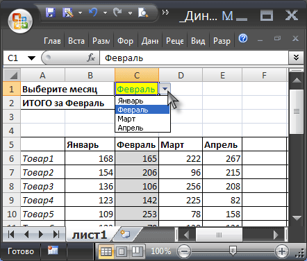
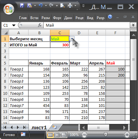
Задача
Имеется таблица продаж по месяцам некоторых товаров (см.
Файл примера
):
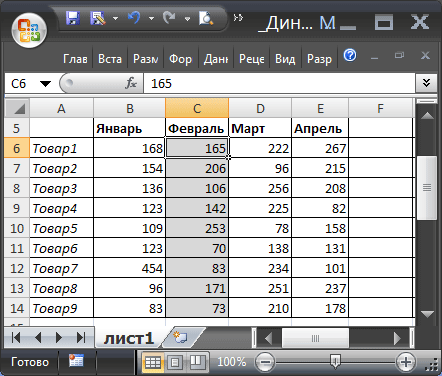
Необходимо найти сумму продаж товаров в определенном месяце. Пользователь должен иметь возможность выбрать нужный ему месяц и получить итоговую сумму продаж. Выбор месяца пользователь должен осуществлять с помощью
Выпадающего списка
.
Для решения задачи нам потребуется сформировать два
динамических диапазона
: один для
Выпадающего списка
, содержащего месяцы; другой для диапазона суммирования.
Для формирования динамических диапазонов будем использовать функцию
СМЕЩ()
, которая возвращает ссылку на диапазон в зависимости от значения заданных аргументов. Можно задавать высоту и ширину диапазона, а также смещение по строкам и столбцам.
Создадим
динамический диапазон
для
Выпадающего списка
, содержащего месяцы. С одной стороны нужно учитывать тот факт, что пользователь может добавлять продажи за следующие после апреля месяцы (май, июнь…), с другой стороны
Выпадающий список
не должен содержать пустые строки.
Динамический диапазон
как раз и служит для решения такой задачи.
Для создания динамического диапазона:
-
на вкладке
Формулы
в группе
Определенные имена
выберите команду
Присвоить имя
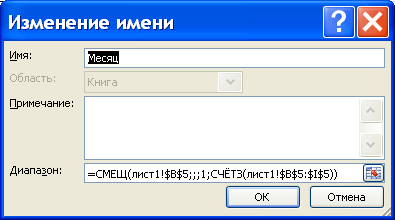
; -
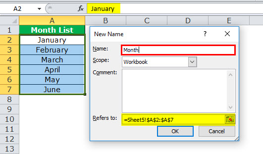
в поле
Имя
введите:
Месяц
; -
в поле
Область
выберите лист
Книга
; -
в поле
Диапазон
введите формулу
=СМЕЩ(лист1!$B$5;;;1;СЧЁТЗ(лист1!$B$5:$I$5))
- нажмите ОК.
Теперь подробнее. Любой диапазон в EXCEL задается координатами верхней левой и нижней правой ячейки диапазона. Исходной ячейкой, от которой отсчитывается положение нашего динамического диапазона, является ячейка
B5
. Если не заданы аргументы функции
СМЕЩ()
смещ_по_строкам,
смещ_по_столбцам
(как в нашем случае), то эта ячейка является левой верхней ячейкой диапазона. Нижняя правая ячейка диапазона определяется аргументами
высота
и
ширина
. В нашем случае значение высоты =1, а значение ширины диапазона равно результату вычисления формулы
СЧЁТЗ(лист1!$B$5:$I$5)
, т.е. 4 (в строке 5 присутствуют 4 месяца с
января
по
апрель
). Итак, адрес нижней правой ячейки нашего
динамического диапазона
определен – это
E
5
.
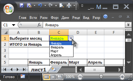
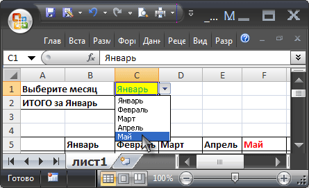
При заполнении таблицы данными о продажах за
май
,
июнь
и т.д., формула
СЧЁТЗ(лист1!$B$5:$I$5)
будет возвращать число заполненных ячеек (количество названий месяцев) и соответственно определять новую ширину динамического диапазона, который в свою очередь будет формировать
Выпадающий список
.
ВНИМАНИЕ! При использовании функции
СЧЕТЗ()
необходимо убедиться в отсутствии пустых ячеек! Т.е. нужно заполнять перечень месяцев без пропусков.
Теперь создадим еще один
динамический диапазон
для суммирования продаж.
Для создания
динамического диапазона
:
-
на вкладке
Формулы
в группе
Определенные имена
выберите команду
Присвоить имя
; -
в поле
Имя
введите:
Продажи_за_месяц
; -
в поле
Диапазон
введите формулу =
СМЕЩ(лист1!$A$6;;ПОИСКПОЗ(лист1!$C$1;лист1!$B$5:$I$5;0);12)
- нажмите ОК.
Теперь подробнее.
Функция
ПОИСКПОЗ()
ищет в строке 5 (перечень месяцев) выбранный пользователем месяц (ячейка
С1
с выпадающим списком) и возвращает соответствующий номер позиции в диапазоне поиска (названия месяцев должны быть уникальны, т.е. этот пример не годится для нескольких лет). На это число столбцов смещается левый верхний угол нашего динамического диапазона (от ячейки
А6
), высота диапазона не меняется и всегда равна 12 (при желании ее также можно сделать также динамической – зависящей от количества товаров в диапазоне).
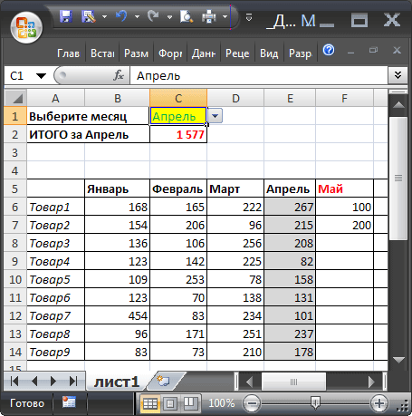
И наконец, записав в ячейке
С2
формулу =
СУММ(Продажи_за_месяц)
получим сумму продаж в выбранном месяце.
Например, в мае.
Или, например, в апреле.
Примечание:
Вместо формулы с функцией
СМЕЩ()
для подсчета заполненных месяцев можно использовать формулу с функцией
ИНДЕКС()
: =
$B$5:ИНДЕКС(B5:I5;СЧЁТЗ($B$5:$I$5))
Формула подсчитывает количество элементов в строке 5 (функция
СЧЁТЗ()
) и определяет ссылку на последний элемент в строке (функция
ИНДЕКС()
), тем самым возвращает ссылку на диапазон
B5:E5
.
Визуальное отображение динамического диапазона
Выделить текущий
динамический диапазон
можно с помощью
Условного форматирования
. В
файле примера
для ячеек диапазона
B6:I14
применено правило
Условного форматирования
с формулой: =
СТОЛБЕЦ(B6)=СТОЛБЕЦ(Продажи_за_месяц)
Условное форматирование
автоматически выделяет серым цветом продажи
текущего месяца
, выбранного с помощью
Выпадающего списка
.
Применение динамического диапазона
Примеры использования
динамического диапазона
, например, можно посмотреть в статьях
Динамические диаграммы. Часть5: график с Прокруткой и Масштабированием
и
Динамические диаграммы. Часть4: Выборка данных из определенного диапазона
.
What do You Mean by Excel Dynamic Named Range?
Dynamic named range in Excel is the ranges that change as the data in the range changes, and the dashboard or charts or reports associated with them. So that is why it is called dynamic. So we can name the range from the name box, so the name is a dynamic name range. So, for example, to make a table as a dynamic named range, we must select the “Data,” insert a table and then name the table.
Table of contents
- What do You Mean by Excel Dynamic Named Range?
- How to Create Excel Dynamic Named Range? (Step by Step)
- Rules for Creating Dynamic Named Range in Excel
- Recommended Articles
How to Create Excel Dynamic Named Range? (Step by Step)
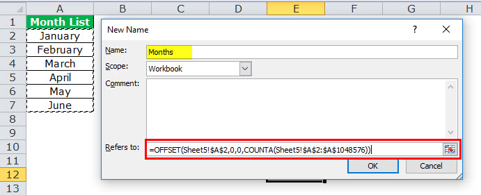
Below are steps to create an Excel dynamic named range:
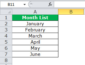
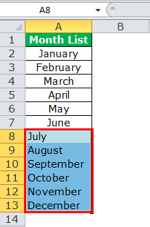
- We must first create a list of months from Jan to Jun.

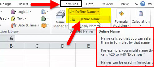
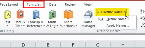
- Then, we need to go to the “Define Name” tab.

- Click on that and give a name to it.

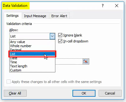
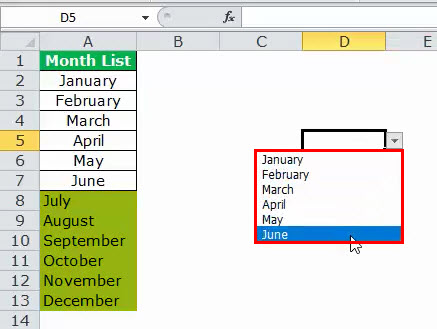
- After that, we must create data validation for the month list.

- Click on the “data validation“, and the below box will open.

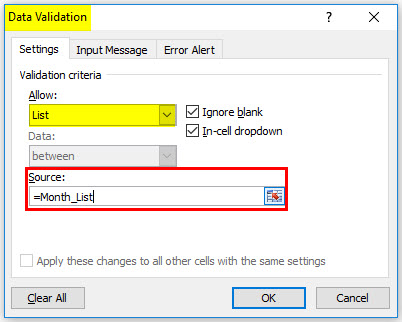
- Select the “List” from the drop-down.

- Select the”List,” and in “Source, ” we must give the name defined for the month list.

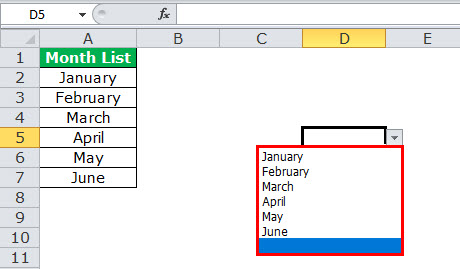
- Now, the drop-down list has been created.

- After that, we need to add the remaining six months to the list.

- Now, return and check the drop-down list we have created in the previous step. It shows only the first six months. Whatever we have added later, it will not display.

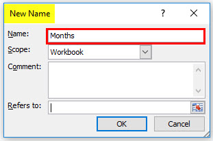
- We must define a new name now under the “Define Name” section.

- Give a name to your list and select the range.

- Under the “Refers to” section, we must apply the formula as shown in the below image.

- Now, return and check the drop-down list we have created in the previous step. Now, it shows all the 12 months in the drop-down list. We can see everything in that column.
“Name Manager” would dynamically update the dropdown list whenever the data expands.


Rules for Creating Dynamic Named Range in Excel
It will help if we consider certain things while defining the names. But, first, we must follow the below rules from Microsoft, which are pre-determined.
- The first letter of the name should begin with a letter or underscore (_) or backslash ()
- We cannot give any space in between two words.
- We cannot provide a cell referenceCell reference in excel is referring the other cells to a cell to use its values or properties. For instance, if we have data in cell A2 and want to use that in cell A1, use =A2 in cell A1, and this will copy the A2 value in A1.read more as our name, for example, A50, B10, C55, etc.
- We cannot use letters like C, c, R, and r because Excel uses them as selection shortcuts.
- “Define Name” is not case-sensitive. MONTHS and months both are the same.
Recommended Articles
This article has been a guide to a dynamic named range in Excel. Here, we discuss creating a dynamic range in Excel and practical examples and downloadable templates. You may learn more about Excel from the following articles: –
- VBA Range
- Dynamic Chart in Excel
- Excel Dynamic Table
- Use INDEX Excel Function
- Excel Date Picker
In my recent article, I talked all about named ranges in excel. While exploring named ranges, the topic of dynamic ranged popped up. So in this article, I will explain, how can you make Dynamic Range in Excel.

What is Dynamic Named Range in Excel?
A normal named range is static. If you define C2:C10 as Item, Item will always refer to C2:C10, until and unless you edit it manually. In below image, we are counting blanks in the Item list. It is showing 2. If it were dynamic it would have shown 0.
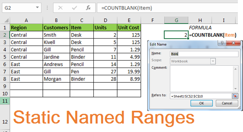
A dynamic name range is name range that expands and shrinks according to data. For example if you have a list of items in range C2:C10 and name it Items, it should expand itself to C2:C11 if you add a new item in range and should shrink if you reduce when you delete as above.
How to Create A Dynamic Name Range
Create Named Ranges Using Excel Tables
Yes, excel tables can make dynamic named ranges. They will make each column in a table named range that is highly dynamic.
But there is one drawback of table names that you can’t use them in Data Validation and Conditional Formatting. But specific Named ranges can be used there.
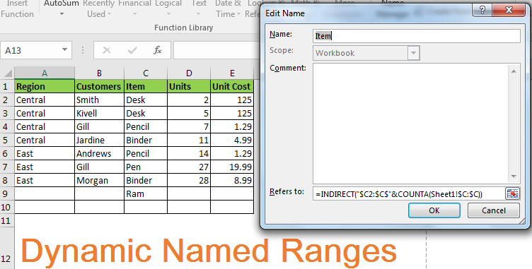
Use INDIRECT and COUNTA Formula
To make a name range dynamic, we can use INDIRECT and COUNTA function
. How? Lets see.
Generic Formula to be written in Refers To: section
=INDIRECT(«$startingCell:$endingColumnLetter$»&COUNTA($columnLetter:$columnLetter))
Above generic formula may look complex but it is easy actually. Let’s see by an example.
The basic idea is to determine last used cell.
Dynamic Range Example
In above example we had an static name range Item in range C2:C10. Let’s make it dynamic.
-
- Open Name Manager by Pressing CTRL+F3.
- Now if a name already exists on the range, click on it and then click edit. Else click on New.
- Name it Item.
- In Refers To: Section write Below Formula.
- Hit OK Button.
And it’s done. Now, whenever you will type Item in name box or in any formula it will refer to C2 to last used cell in the range.
Caution: No cell should be blank in-between range. Otherwise, the range will be reduced by the number of blank cells.
How does it work?
As I said, its only matter finding last used cell. For this example, no cells should be blank in between. Why? You’ll Know.
INDIRECT function in excel converts a text into range. =INDIRECT(“$C$2:$C$9”) will refer to absolute range $C$2:$C$10. We just need to find the last row number dynamically (9).
Since all cells have some value in range C2:C10, we can use COUNTA function to find the last row.
So,=INDIRECT(«$C2:$C$»& this part fixes the starting row and column and COUNTA($C:$C) dynamical calculates last used row.
So yeah, this is how you can make the most effective Dynamic Named Ranges that will work with every formula and functionality of Excel. You don’t need to edit your named range again when you change data.
Download file:
Related Article:
How to use Named Ranges in Excel
17 Amazing Features of Excel Tables
Popular Articles:
50 Excel Shortcuts to Increase Your Productivity
How to use the VLOOKUP Function in Excel
How to use the COUNTIF function in Excel
How to use the SUMIF Function in Excel