Excel for Microsoft 365 Excel for Microsoft 365 for Mac Excel for the web Excel 2021 Excel 2021 for Mac Excel 2019 Excel 2019 for Mac Excel 2016 Excel 2016 for Mac Excel 2013 Excel 2010 Excel 2007 Excel for Mac 2011 Excel Starter 2010 More…Less
This article describes the formula syntax and usage of the DSUM function in Microsoft Excel.
Description
Adds the numbers in a field (column) of records in a list or database that match conditions that you specify.
Syntax
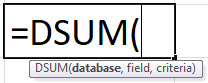
DSUM(database, field, criteria)
The DSUM function syntax has the following arguments:
-
Database Required. The range of cells that makes up the list or database. A database is a list of related data in which rows of related information are records, and columns of data are fields. The first row of the list contains labels for each column.
-
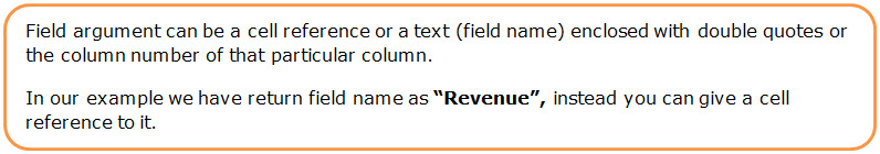
Field Required. Indicates which column is used in the function. Enter the column label enclosed between double quotation marks, such as «Age» or «Yield,» or a number (without quotation marks) that represents the position of the column within the list: 1 for the first column, 2 for the second column, and so on.
-
Criteria Required. Is the range of cells that contains the conditions that you specify. You can use any range for the criteria argument, as long as it includes at least one column label and at least one cell below the column label in which you specify a condition for the column.
Remarks
-
You can use any range for the criteria argument, as long as it includes at least one column label and at least one cell below the column label for specifying the condition.
For example, if the range G1:G2 contains the column label Income in G1 and the amount $10,000 in G2, you could define the range as MatchIncome and use that name as the criteria argument in the database functions.
-
Although the criteria range can be located anywhere on the worksheet, do not place the criteria range below the list. If you add more information to the list, the new information is added to the first row below the list. If the row below the list is not blank, Microsoft Excel cannot add the new information.
-
Make sure that the criteria range does not overlap the list.
-
To perform an operation on an entire column in a database, enter a blank line below the column labels in the criteria range.
Example
Copy the example data in the following table, and paste it in cell A1 of a new Excel worksheet. For formulas to show results, select them, press F2, and then press Enter. If you need to, you can adjust the column widths to see all the data.
|
Tree |
Height |
Age |
Yield |
Profit |
Height |
|---|---|---|---|---|---|
|
=»=Apple» |
>10 |
<16 |
|||
|
=»=Pear» |
|||||
|
Tree |
Height |
Age |
Yield |
Profit |
|
|
Apple |
18 |
20 |
14 |
$105 |
|
|
Pear |
12 |
12 |
10 |
$96 |
|
|
Cherry |
13 |
14 |
9 |
$105 |
|
|
Apple |
14 |
15 |
10 |
$75 |
|
|
Pear |
9 |
8 |
8 |
$77 |
|
|
Apple |
8 |
9 |
6 |
$45 |
|
|
Formula |
Description |
Result |
|||
|
=DSUM(A4:E10,»Profit»,A1:A2) |
The total profit from apple trees (rows 5, 8, and 10). |
$225 |
|||
|
=DSUM(A4:E10,»Profit», A1:F3) |
The total profit from apple trees with a height between 10 and 16 feet, and all pear trees (rows 6, 8, and 9). |
$248 |
Top of Page
Need more help?
Want more options?
Explore subscription benefits, browse training courses, learn how to secure your device, and more.
Communities help you ask and answer questions, give feedback, and hear from experts with rich knowledge.
What is DSUM in Excel?
The function DSUM in Excel is also known as the DATABASE SUM function in Excel, which is used to calculate the sum of the given database based on a certain field and provided criteria. This function takes three arguments as inputs: the range for the database, an argument for the field, and a condition, and then it calculates the sum for it.
For example, suppose we have a dataset with an order number greater than 100 and the quantity equal to or greater than 10. We need to determine the total number of records. In such a scenario, using the DSUM function in Excel, we can calculate the sum of such orders.
Table of contents
- What is DSUM in Excel?
- Syntax
- How to Use the DSUM Function in Excel?
- How does DSUM Work?
- Practical DSUM Examples
- Q1 – Our first question is to calculate the revenue for the region “Central.”
- Q-2: Calculate total revenue for the region “East” for the item “Pen.”
- Q-3: Sum of sales for all the Rep other than Gill.
- Q-4: Sum of sales for units greater than 25.
- Q-5: Sum of sales from 18th Oct 2014 to 17th Oct 2015
- Q-6: Sum of sales for Rep Smith, for item Binder, for Region Central
- Things to Remember
- Recommended Articles
Syntax
Below is the DSUM Formula in Excel:
- Database: It is simply the data table along with headers.
- Field: The column you would like to sum in the data table. i.e., column header.
- Criteria: List of criteria in the cells containing the conditions specified by the user.
How to Use the DSUM Function in Excel?
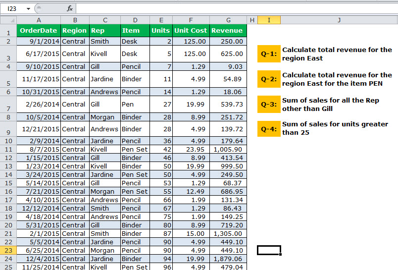
The below image shows the sale of stationery items, and we have some requirements to calculate. We have five different situations to calculate the revenue. Each situation is not a different situation but conditions that we need to implement.
The DSUM is a criteria-based function that can return the value based on your criteria. It will give you the sum of the column based on multiple requirements. For example, total sales for the salesperson in the region west for the product desk. So it is a bit of a SUMIFS kind of functionThe SUMIF Excel function calculates the sum of a range of cells based on given criteria. The criteria can include dates, numbers, and text. For example, the formula “=SUMIF(B1:B5, “<=12”)” adds the values in the cell range B1:B5, which are less than or equal to 12.
read more. Based on certain criteria, it will return the value.
How does DSUM Work?
The word database is not a stranger to excelling users. In Excel for the database, we use the word range of cells or cells or tables, etc. As we mentioned earlier in the article, the DSUM is a database function based on the criteria we express in a range of cells following the same database or table structure. We can give criteria to each column by mentioning it as a header and the given criteria under it.
If you already know how SUMIF and SUMIFS work, then DSUM should not be a complex thing to understand.
Let us learn ahead to get an idea about the functionality of the DSUM function.
Practical DSUM Examples
You can download this DSUM Function Excel template here – DSUM Function Excel template
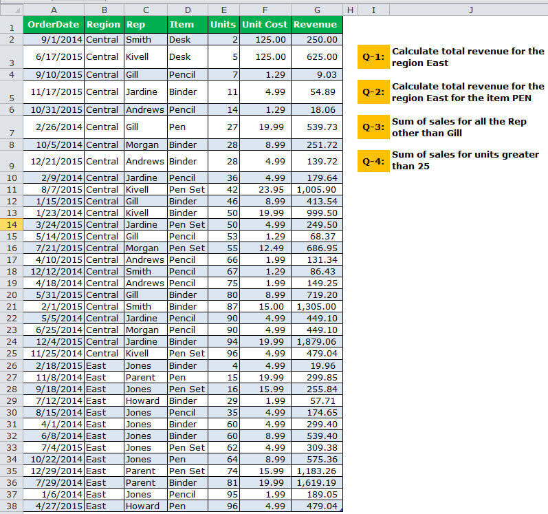
Look at the below image where we have sales data from A1 to G38. Then, answer all the questions from the below table.
Set up the Data: Since we already have our criteria, we need first to set up the data table. We must select the data and make it in a table format. Then, click the “Ctrl + T” and choose the data.
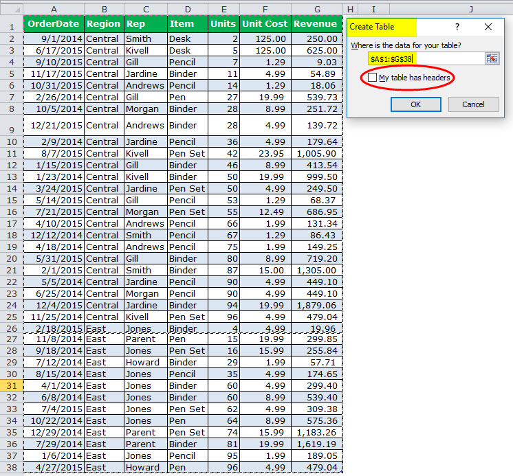
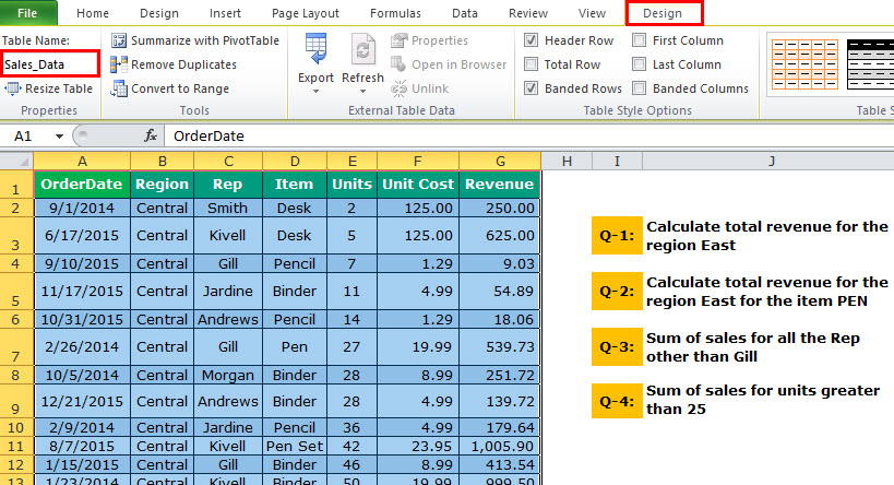
And, name the table “Sales_Data.”
Create Your Criteria: After setting up the table, we need to create our criteria. Our first criteria will be like the one below.
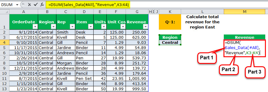
Q1 – Our first question is to calculate the revenue for the region “Central.”

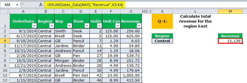
We must apply the DSUM formula to get the region “Central” total.
The output is 11,139.
Part 3: To sum up, we must specify the criteria as the “Central” region.
Part 2: It specifies which column you need to sum, i.e., the “Revenue” column in the table.
Part 1: It is taking the range of databases. We name our database “Sales_Data.”
Note: All the characters should be the same as in the data table for the “criteria” column.
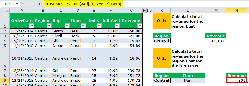
Q-2: Calculate total revenue for the region “East” for the item “Pen.”
We need to calculate the total revenue for the region “East” but only for “Pen” in the item column.
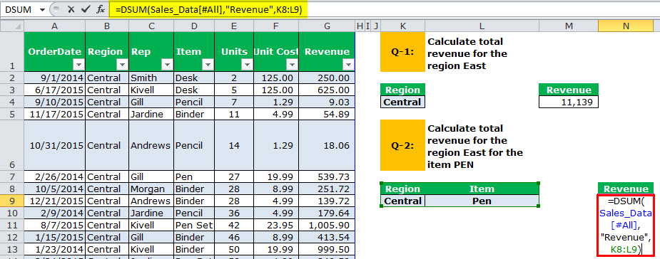
The output is 4,501.
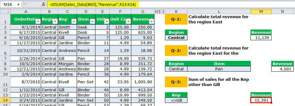
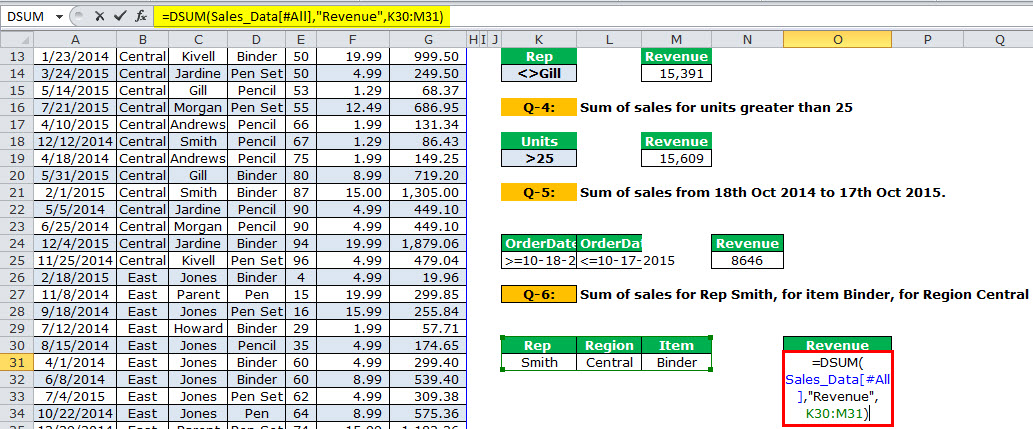
Q-3: Sum of sales for all the Rep other than Gill.
We need to calculate the “Sum for all the Rep other than Gill.” We need to give criteria under “Rep” as <>Gill.
“<>” means not equal to.
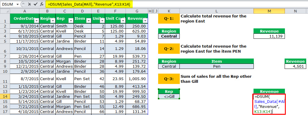
The output is 15,391.
Q-4: Sum of sales for units greater than 25.
The equation calculates the total revenue for all the units greater than 25 units.
For this, set the criteria as >25.
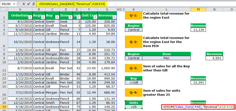
The output is 15,609.

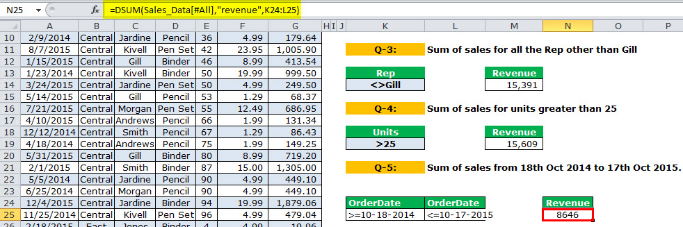
Q-5: Sum of sales from 18th Oct 2014 to 17th Oct 2015
We need to get the total revenue from 18th Oct 2014 to 17th Oct 2015. To do this, we need to set two criteria for one column.
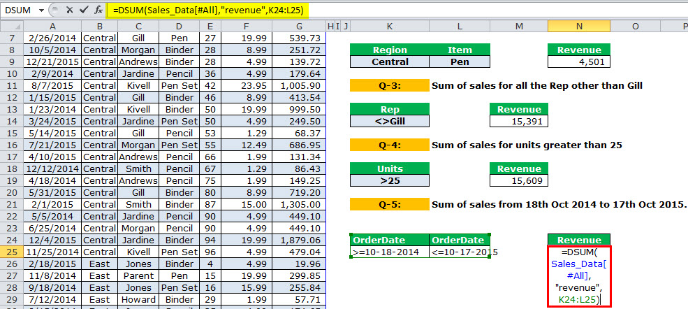
The output is 8646.
Q-6: Sum of sales for Rep Smith, for item Binder, for Region Central
Now, we have to match 3 different criteria to get the total.

We must design the criteria as shown in the below table and apply the DSUM function.
Things to Remember
- While writing a field name, it must be in double quotes and should be as same as in the table header.
- First, identify the criteria requirement and list all the criteria.
- We must create a table for the data. If the data size increases, it will be a dynamic range. You need not worry about the range.
- The #Value error#VALUE! Error in Excel represents that the reference cell the user has either entered an incorrect formula or used a wrong data type (mostly numerical data). Sometimes, it is difficult to identify the kind of mistake behind this error.read more occurs due to wrong field names included in the database argument.
- If we do not give any specific criteria, it will just give us the overall sum for the column.
- We must create a drop-down list of your criteria to get different regions or different rep totals.
- As soon as we change the drop-down list, it may show the results accordingly.
- The criteria table is not case-sensitive.
- It is an alternative formula for SUMIF and SUMIFS functionsSUMIFS is an enhanced version of the SUMIF formula in Excel that enables you to sum any range of data by matching several criteria. read more.
Recommended Articles
This article has been a guide to DSUM in Excel. Here, we discuss the DSUM formula in Excel and how to use the DSUM function in Excel, along with Excel examples and downloadable Excel templates. You may learn more about Excel functions from the following articles: –
- SUM Formula Excel
- Percentile Formula in Excel
- Examples of HLOOKUP
- Excel Reference to Another Sheet
What is the DSUM Function? The DSUM function is categorized under Excel Database functions.The function helps to calculate the sum of a specific field/column in a database for selected records based on user-specified criteria.
Contents
- 1 What does Dsum mean in Excel?
- 2 What does Dsum mean?
- 3 What is the difference between Dsum and Sumif?
- 4 What is Dsum formula?
- 5 How does a DSUM function?
- 6 What is Dsum access?
- 7 How do I use Hlookup?
- 8 What is the difference between Iserror and Iferror?
- 9 What is difference between sum and Sumif?
- 10 What is the difference between Count and Counta?
- 11 What is field in Dsum?
- 12 What is Dsum in Google Sheets?
- 13 How do I use custom AutoFilter in Excel?
- 14 How does Sumif work Excel?
- 15 How do I use Ifsum?
- 16 How do you use the Match function in Excel?
- 17 What is a domain in access?
- 18 How do you sum in access?
- 19 How do you create a running total in access?
- 20 What is macro in Excel?
What does Dsum mean in Excel?
Description. The Microsoft Excel DSUM function sums the numbers in a column or database that meets a given criteria. The DSUM function is a built-in function in Excel that is categorized as a Database Function. It can be used as a worksheet function (WS) in Excel.
What does Dsum mean?
DSUM in excel is also known as DATABASE Sum function in excel which is used to calculate the sum of the given data base based on a certain field and a given criteria, this function takes three arguments as inputs and they are the range for database an argument for field and a condition and then it calculates the sum
What is the difference between Dsum and Sumif?
DSUM finds results based on the given conditions from the whole database that includes the column names. In SUMIFS you can select data from different as well as distant column ranges.That means scattered criteria columns can be included in SUMIFS if they have the same number of rows in comparison to the sum range. 3.
What is Dsum formula?
The DSUM function is categorized under Excel Database functions.The function helps to calculate the sum of a specific field/column in a database for selected records based on user-specified criteria. DSUM was introduced in MS Excel 2000.
How does a DSUM function?
The Excel DSUM function calculates a sum of values in a set of records that match criteria. The values to sum are extracted from a given field in the database, specified as an argument.
Criteria options.
| Criteria | Behavior |
|---|---|
| Re* | Begins with “re” |
| 10 | Equal to 10 |
| >10 | Greater than 10 |
| <> | Not blank |
What is Dsum access?
Description. The Microsoft Access DSum function returns the sum of a set of numeric values from an Access table (or domain).
How do I use Hlookup?
Use HLOOKUP when your comparison values are located in a row across the top of a table of data, and you want to look down a specified number of rows. Use VLOOKUP when your comparison values are located in a column to the left of the data you want to find. The H in HLOOKUP stands for “Horizontal.”
What is the difference between Iserror and Iferror?
Whereas IFERROR assumes that you always want the result if it isn’t an error, ISERROR allows you to specify whether you want the result or something else.
What is difference between sum and Sumif?
The SUM function totals one or more numbers in a range of cells. SUMIF FUNCTION -The SUMIF function is a worksheet function that adds all numbers in a range of cells based on one criteria (for example, is equal to 2000). The SUMIF function is a built-in function in Excel that is categorized as a Math/Trig Function.
What is the difference between Count and Counta?
The difference between them is that COUNT only counts cells containing numbers but COUNTA counts all cells that aren’t empty. Think of it as “Count Anything”.
DSUM(database, field, criteria) The DSUM function syntax has the following arguments: Database Required. The range of cells that makes up the list or database. A database is a list of related data in which rows of related information are records, and columns of data are fields.
What is Dsum in Google Sheets?
The DSUM function is used to find the sum of numbers in a column (of a database-like range) that satisfy a given criteria. In this way, it is a lot like the SUMIFS function.
How do I use custom AutoFilter in Excel?
To use advanced number filters:
- Select the Data tab on the Ribbon, then click the Filter command.
- Click the drop-down arrow for the column you want to filter.
- The Filter menu will appear.
- The Custom AutoFilter dialog box will appear.
- The data will be filtered by the selected number filter.
How does Sumif work Excel?
The SUMIF function returns the sum of cells in a range that meet a single condition. The first argument is the range to apply criteria to, the second argument is the criteria, and the last argument is the range containing values to sum.If you need to apply multiple criteria, use the SUMIFS function.
How do I use Ifsum?
If you want, you can apply the criteria to one range and sum the corresponding values in a different range. For example, the formula =SUMIF(B2:B5, “John”, C2:C5) sums only the values in the range C2:C5, where the corresponding cells in the range B2:B5 equal “John.”
How do you use the Match function in Excel?
The MATCH function searches for a specified item in a range of cells, and then returns the relative position of that item in the range. For example, if the range A1:A3 contains the values 5, 25, and 38, then the formula =MATCH(25,A1:A3,0) returns the number 2, because 25 is the second item in the range.
What is a domain in access?
An access domain is a unique hostname that is assigned to a particular service. It will always resolve to your service, regardless of whether any other domains have DNS pointing to the service.An access domain is a unique hostname that is assigned to a particular service.
How do you sum in access?
On the Home tab, in the Records group, click Totals. A new Total row appears in your datasheet. In the Total row, click the cell in the field that you want to sum, and then select Sum from the list.
How do you create a running total in access?
Create a query with the Transaction table as the source, and add the Debits field. Click the Totals button so the line appears in the design grid, and set it to Sum. Save the query as “Total.” Now we’re ready to calculate the running totals and the percent of total.
What is macro in Excel?
If you have tasks in Microsoft Excel that you do repeatedly, you can record a macro to automate those tasks. A macro is an action or a set of actions that you can run as many times as you want. When you create a macro, you are recording your mouse clicks and keystrokes.

This Excel tutorial explains how to use the Excel DSUM function with syntax and examples.
Description
The Microsoft Excel DSUM function sums the numbers in a column or database that meets a given criteria.
The DSUM function is a built-in function in Excel that is categorized as a Database Function. It can be used as a worksheet function (WS) in Excel. As a worksheet function, the DSUM function can be entered as part of a formula in a cell of a worksheet.
Syntax
The syntax for the DSUM function in Microsoft Excel is:
DSUM( range, field, criteria )
Parameters or Arguments
- range
- The range of cells that you want to apply the criteria against.
- field
- The column to sum the values. You can either specify the numerical position of the column in the list or the column label in double quotation marks.
- criteria
- The range of cells that contains your criteria.
Returns
The DSUM function returns a numeric value.
Applies To
- Excel for Office 365, Excel 2019, Excel 2016, Excel 2013, Excel 2011 for Mac, Excel 2010, Excel 2007, Excel 2003, Excel XP, Excel 2000
Type of Function
- Worksheet function (WS)
Example (as Worksheet Function)
Let’s look at some Excel DSUM function examples and explore how to use the DSUM function as a worksheet function in Microsoft Excel:
Based on the Excel spreadsheet above, the following DSUM examples would return:
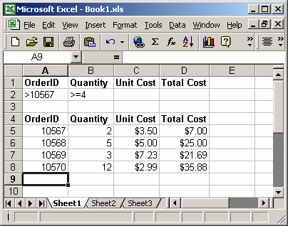
=DSUM(A4:D8, "Unit Cost", A1:B2)
Result: 7.99
Let’s quickly explain why the DSUM function returns 7.99 in this example. The criteria for the DSUM calculation is found in cells A1:B2. This means that only those records where the order number is greater than 10567 and Quantity is greater than equal to 4 will be included in the sum calculations.
So in the example above, only rows 6 and 8 meet those conditions. As a result, the DSUM adds together the Unit Cost values in only rows 6 and 8 to return 7.99 (5.00 + 2.99).
Here are some more examples of the DSUM function:
=DSUM(A4:D8, 3, A1:B2)
Result: 7.99

=DSUM(A4:D8, "Quantity", A1:A2)
Result: 20

=DSUM(A4:D8, 2, A1:A2)
Result: 20
Using Named Ranges
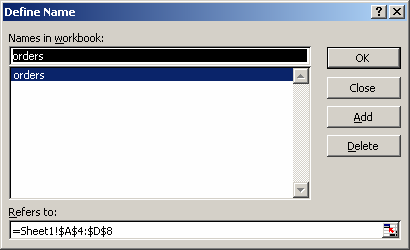
You can also use a named range in the DSUM function. A named range is a descriptive name for a collection of cells or range in a worksheet. If you are unsure of how to setup a named range in your spreadsheet, read our tutorial on Adding a Named Range.
For example, we’ve created a named range called orders that refers to Sheet1!$A$4:$D$8.
Then we’ve entered the following data in Excel:
Based on the Excel spreadsheet above, the following DSUM examples would return:
=DSUM(orders, "Total Cost", A1:B2)
Result: 60.88

=DSUM(orders, 4, A1:B2)
Result: 60.88
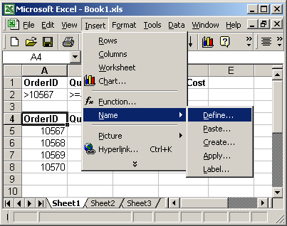
To view named ranges: Under the Insert menu, select Name > Define.