
Содержание
- Discount
- Calculate Percentage Discount
- Calculate Discounted Price
- Calculate Original Price
- How to Calculate a Discount Rate in Excel
- Key Takeaways
- Discount Rate
- =RATE (nper, pmt, pv, [fv], [type], [guess])
- Calculating the Discount Rate in Excel
- Method One
- Method Two
- Discount Factor
- Discount Rate
- Discount Factor
- What Is the Formula for the Discount Rate?
- What Does the Discount Rate Indicate?
- What Is Net Present Value?
- Calculators
- Online calculators to make your life easier
- Calculate Discount in Excel
- Formula to find out the discount value
- Other forms of calculating discount in Excel
- Discount Factor Table for Excel
- What is a Discount Factor?
- Cash Flow Diagrams
- Discount Rate
- Monthly Payment Periods (p=12)
- Daily Compounding (p=365 or p=360)
- Discount Factor Table for Discrete Compounding
- Discount Factors for Continuous Compounding
Discount
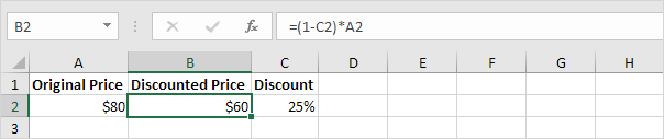
If you know the original price and the discounted price, you can calculate the percentage discount. If you know the original price and the percentage discount, you can calculate the discounted price, etc.
Calculate Percentage Discount
If you know the original price and the discounted price, you can calculate the percentage discount.
1. First, divide the discounted price by the original price.
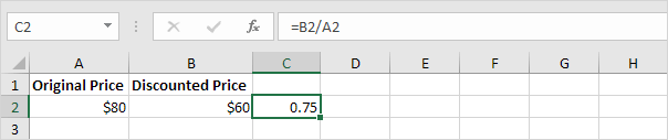
Note: you’re still paying $60 of the original $80. This equals 75%.
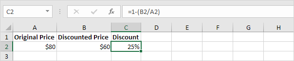
2. Subtract this result from 1.

Note: if you’re still paying 75%, you’re not paying 25% (the percentage discount).
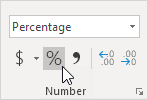
3. On the Home tab, in the Number group, click the percentage symbol to apply a Percentage format.
Calculate Discounted Price
If you know the original price and the percentage discount, you can calculate the discounted price.
1. First, subtract the percentage discount from 1.
Note: you’re still paying 75%.
2. Multiply this result by the original price.
Note: you’re still paying 75% of the original $80. This equals $60.
Calculate Original Price
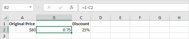
If you know the discounted price and the percentage discount, you can calculate the original price. Take a look at the previous screenshot. To calculate the discounted price, we multiplied the original price by (1 — Percentage Discount).
1. To calculate the original price, simply divide the discounted price by (1 — Percentage Discount).
Источник
How to Calculate a Discount Rate in Excel
:max_bytes(150000):strip_icc()/nicklioudis__nick_lioudis-5bfc261b46e0fb00265aeabe.jpg)
:max_bytes(150000):strip_icc()/IMG_7291_Crop-SomerAnderson-fdd793749683441487bbf0bd73328c59.jpg)
:max_bytes(150000):strip_icc()/2G8T0126-BW-5a525a4d8c434885b365bee7b3807f60.jpg)
For discounted cash flow analysis, the discount rate refers to the interest rate used when calculating the net present value (NPV) of an investment. It represents the time value of money.
NPV is a core component of corporate budgeting and is a comprehensive way to calculate whether a proposed project will add value or not.
For this article, when we look at the discount rate, we will be solving for the rate that results in the NPV equaling zero. Doing so allows us to determine the internal rate of return (IRR) of a project or asset.
Key Takeaways
- The discount rate is the interest rate used to calculate net present value.
- It represents the time value of money.
- Net present value can help companies to determine whether a proposed project may be profitable.
- Net present value is essential to corporate budgeting.
- For an NPV of zero, Excel can find the internal rate of return and use that as the discount rate.
Discount Rate
First, let’s examine each step of NPV in order. The formula is:
Broken down, each period’s after-tax cash flow at time t is discounted by some rate, shown as r. The sum of all these discounted cash flows is then offset by the initial investment, which equals the current NPV. Any NPV greater than $0 is a value-added project.
In the decision-making process relating to competing yet comparable projects, a project with the highest NPV should tip the scale toward its selection.
The IRR is the discount rate that makes the NPV of future cash flows equal to zero.
The NPV, IRR, and discount rate are all connected concepts. With an NPV, you know the amount and timing of cash flows. You also know the weighted average cost of capital (WACC), which is designated as r when solving for the NPV. With an IRR, you know the same details, and you can solve for the NPV expressed as a percentage return.
The question is, what is the discount rate that sets the IRR to zero? This is the same rate that will give the NPV a value of zero. As you will see below, if the discount rate equals the IRR, then the NPV is zero. Or to put it another way, if the cost of capital equals the return of capital, then the project will break even and have an NPV of 0.
=RATE (nper, pmt, pv, [fv], [type], [guess])
The Excel formula for calculating the discount rate. It’s often used to calculate the interest rate for a loan or to determine the rate of return required to meet a particular investment objective.
Calculating the Discount Rate in Excel
In Excel, you can solve for the discount rate in two ways:
- You can find the IRR and use that as the discount rate, which causes NPV to equal zero.
- You can use What-If analysis, a built-in calculator in Excel, to solve for the discount rate that equals zero.
Method One
To illustrate the first method, we will take our NPV/IRR example. Using a hypothetical outlay, our WACC risk-free rate, and expected after-tax cash flows, we’ve calculated an NPV of $472,169 with an IRR of 57%.
We’ve already defined the discount rate as a WACC that causes the IRR to equal 0. So, we can just take our calculated IRR and put it in place of WACC to get the NPV of 0. That calculation is shown below:
Method Two
Let’s now look at the second method, using Excel’s What-If calculator. This assumes that we did not calculate the IRR of 57%, as we did above, and have no idea what the correct discount rate is.
To get to the What-If solver, go to the Data Tab —> What-If Analysis Menu —> Goal Seek. Then simply plug in the numbers and Excel will solve for the correct value. When you select «OK,» Excel will recalculate WACC to equal the discount rate that makes the NPV zero (57%).
Discount Factor
When working with the discount rate, you may come across the discount factor, as well. They aren’t the same thing although they may be used together in calculations. The discount factor, when multiplied by a cash flow value, discounts that value and provides a present value.
It’s used by Excel to shed added light on the NPV formula and the impact that discounting can have.
Here’s a comparison of the discount rate and the discount factor.
Discount Rate
- Along with time period, it’s used in the formula that calculates the discount factor.
- It represents the time value of money.
- It’s a rate of return determined by a company.
- It’s used in the calculation of present value.
Discount Factor
- As the discount rate increases due to compounding over time, the discount factor increases.
- It facilitates audits of a discounted cash flow model.
- It illustrates the effect of compounding.
- It’s an alternative to using the XNPV and XIRR functions in Excel.
What Is the Formula for the Discount Rate?
The formula for calculating the discount rate in Excel is =RATE (nper, pmt, pv, [fv], [type], [guess]).
What Does the Discount Rate Indicate?
The discount rate represents an interest rate. In discounted cash flow analysis, it’s used in the calculation of the present value of future money. It can tell you the amount of money you’d need today to earn a certain amount in the future.
What Is Net Present Value?
It’s the difference between the present value of cash flows and the present value of cash outlays. It’s used by businesses for corporate budgeting and can help them determine the potential profitability of a proposed project or investment.
Источник
Calculators
Online calculators to make your life easier
Calculate Discount in Excel
Learn how to easily find out the discount percentage of any product using this simple Excel formula. Calculate the final value by applying the discount!
One of the most useful formulas to use in spreadsheets is for discount percentages. With this formula you can easily find out the final value by applying any amount of discount to any price.
Formula to find out the discount value
There are several ways of discovering a discount percentage for any value but the most simple is:
discounted value = (discount percentage * total value) / 100
For example, if you would like to know the discounted value of something that costs €3,000 and has a discount of 15%:
(15 * 3000) / 100 = 450
To understand the formula in terms of cells, where the percentage is placed in cell A1 and the price in cell A2:
Finally, if you want to know the final cost of a product, simply subtract the amount of the discount from the initial amount:
final value (with discount applied) = initial value — ((discount percentage * total value)/100)
Other forms of calculating discount in Excel
If you prefer, here you will find other formulas for calculating percentages using Excel or any other type of spreadsheet.
Источник
Discount Factor Table for Excel
A discount factor can be thought of as a conversion factor for time value of money calculations. The discount factor table below provides both the mathematical formulas and the Excel functions used to convert between present value (P), future worth (F), uniform gradient amount (G), and uniform series or annuity amount (A).
What is a Discount Factor?
Time value of money calculations are based on the principle that funds placed in a secure investment earn interest over time. The compounding principle states that if we have $P to invest now, the future value will increase to $F=$P*(1+i) n after n years, where i is the effective annual interest rate.
The discounting principle states that if we want to have $F in n years, we need to invest $P right now. So, discounting is basically just the inverse of compounding: $P=$F*(1+i) -n .
The discount formula can be written as P=F*(P/F,i%,n), where (P/F,i%,n) is the symbol used to define the discount factor. To convert the future value to the equivalent present value, you simply multiple the future value by the discount factor.
In the past, it was common to refer to a discount factor table to look up the number needed to perform a time value of money conversion. With the use of calculators and spreadsheets, the table lookup technique is practically obsolete.
Cash Flow Diagrams
A Cash Flow Diagram can help you visualize a series of receipts (positive values) and disbursements (negative values) at discrete periods in time. To be clear about the nomenclature used in the discount factor table, refer to the following cash flow diagrams for P, F, A, and G.
Discount Rate
The Discount Rate, i%, used in the discount factor formulas is the effective rate per period. It uses the same basis for the period (annual, monthly, etc.) as used for the number of periods, n. If only a nominal interest rate (rate per annum or rate per year) is known, you can calculate the discount rate using the following formula:
This formula for the effective rate per period is more general than the formula used in the Excel functions EFFECT and NOMINAL. The EFFECT and NOMINAL functions are only used for converting between the effective and nominal annual rates, where p=1.
Monthly Payment Periods (p=12)
If the compound period is also monthly, the discount rate for a monthly payment period (p=12) simplifies down to i = r / 12. To determine the discount rate for monthly periods with semi-annual compounding, set k=2 and p=12.
Daily Compounding (p=365 or p=360)
The above formula can be used to calculate an effective annual interest rate for daily compounding by setting p=1 and k to the number of banking days in the year (typically 365 or 360).
Discount Factor Table for Discrete Compounding
The following table lists discount factors used for conversions between common discrete cash flow series, present value, future worth, etc. The < >braces around the Excel formula indicate that the formula must be entered as an array function using Ctrl+Shift+Enter.
Example: To convert F to P, multiply F by the discount factor (P/F,i%,n). It might help to think of «P/F» as «P given F». This representation comes from the algebraic equivalence P=F*(P/F).
| Nomenclature | |
|---|---|
| i | Discount Rate (effective rate per period) |
| n | Number of Periods |
| P | Present Worth |
| F | Future Worth |
| A | Uniform Series Amount (or «Annuity») |
| G | Uniform Gradient Amount |
| Convert | Symbol | Discount Factor Formula | Discount Factor Formula in Excel |
|---|---|---|---|
| P to F | (F/P,i%,n) | (1+i) n | =FV(i,n,0,-1) |
| F to P | (P/F,i%,n) | (1+i) -n | =PV(i,n,0,-1) |
| F to A | (A/F,i%,n) | i/((1+i) n -1) | =PMT(i,n,0,-1) |
| P to A | (A/P,i%,n) | i*(1+i) n /((1+i) n -1) | =PMT(i,n,-1) |
| A to F | (F/A,i%,n) | ((1+i) n -1)/i | =FV(i,n,-1) |
| A to P | (P/A,i%,n) | ((1+i) n -1)/(i*(1+i) n ) | =PV(i,n,-1) |
| G to P | (P/G,i%,n) | ((1+i) n -1)/(i 2 *(1+i) n )-n/(i*(1+i) n ) | |
| G to F | (F/G,i%,n) | ((1+i) n -1)/i 2 -(n/i) | <=(P/G,i%,n) * (F/P,i%,n)> |
| G to A | (A/G,i%,n) | (1/i)-n/((1+i) n -1) | <=(P/G,i%,n) * (A/P,i%,n)> |
| EG to P | (P/EG,z-1,n) | (z n -1)/(z n (z-1)), z=(1+i)/(1+g) | =PV(z-1,n,-1) |
The Excel formulas for (F/G,i%,n) and (A/G,i%,n) are based on the algebraic equivalence of F/G=(P/G)*(F/P) and A/G=(P/G)*(A/P). Replace the discount factor symbols (P/G,i%,n), (F/P,i%,n) and (A/P,i%,n) with the appropriate discount factor formula listed in the table.
Discount Factors for Continuous Compounding
Continuous compounding is not exactly the same as daily compounding. The exact discount factor formulas for continuous compounding are given in the table below (where n is the number of years and r is the nominal annual rate). Note that the discount factor for F to P is just the inverse (1/x) of the factor for P to F.
Источник
For discounted cash flow analysis, the discount rate refers to the interest rate used when calculating the net present value (NPV) of an investment. It represents the time value of money.
NPV is a core component of corporate budgeting and is a comprehensive way to calculate whether a proposed project will add value or not.
For this article, when we look at the discount rate, we will be solving for the rate that results in the NPV equaling zero. Doing so allows us to determine the internal rate of return (IRR) of a project or asset.
Key Takeaways
- The discount rate is the interest rate used to calculate net present value.
- It represents the time value of money.
- Net present value can help companies to determine whether a proposed project may be profitable.
- Net present value is essential to corporate budgeting.
- For an NPV of zero, Excel can find the internal rate of return and use that as the discount rate.
Discount Rate
First, let’s examine each step of NPV in order. The formula is:
NPV = ∑ {After-Tax Cash Flow / (1+r)^t} — Initial Investment
Broken down, each period’s after-tax cash flow at time t is discounted by some rate, shown as r. The sum of all these discounted cash flows is then offset by the initial investment, which equals the current NPV. Any NPV greater than $0 is a value-added project.
In the decision-making process relating to competing yet comparable projects, a project with the highest NPV should tip the scale toward its selection.
The IRR is the discount rate that makes the NPV of future cash flows equal to zero.
The NPV, IRR, and discount rate are all connected concepts. With an NPV, you know the amount and timing of cash flows. You also know the weighted average cost of capital (WACC), which is designated as r when solving for the NPV. With an IRR, you know the same details, and you can solve for the NPV expressed as a percentage return.
The question is, what is the discount rate that sets the IRR to zero? This is the same rate that will give the NPV a value of zero. As you will see below, if the discount rate equals the IRR, then the NPV is zero. Or to put it another way, if the cost of capital equals the return of capital, then the project will break even and have an NPV of 0.
=RATE (nper, pmt, pv, [fv], [type], [guess])
The Excel formula for calculating the discount rate. It’s often used to calculate the interest rate for a loan or to determine the rate of return required to meet a particular investment objective.
Calculating the Discount Rate in Excel
In Excel, you can solve for the discount rate in two ways:
- You can find the IRR and use that as the discount rate, which causes NPV to equal zero.
- You can use What-If analysis, a built-in calculator in Excel, to solve for the discount rate that equals zero.
Method One
To illustrate the first method, we will take our NPV/IRR example. Using a hypothetical outlay, our WACC risk-free rate, and expected after-tax cash flows, we’ve calculated an NPV of $472,169 with an IRR of 57%.
We’ve already defined the discount rate as a WACC that causes the IRR to equal 0. So, we can just take our calculated IRR and put it in place of WACC to get the NPV of 0. That calculation is shown below:
Method Two
Let’s now look at the second method, using Excel’s What-If calculator. This assumes that we did not calculate the IRR of 57%, as we did above, and have no idea what the correct discount rate is.
To get to the What-If solver, go to the Data Tab —> What-If Analysis Menu —> Goal Seek. Then simply plug in the numbers and Excel will solve for the correct value. When you select «OK,» Excel will recalculate WACC to equal the discount rate that makes the NPV zero (57%).
Discount Factor
When working with the discount rate, you may come across the discount factor, as well. They aren’t the same thing although they may be used together in calculations. The discount factor, when multiplied by a cash flow value, discounts that value and provides a present value.
It’s used by Excel to shed added light on the NPV formula and the impact that discounting can have.
Here’s a comparison of the discount rate and the discount factor.
Discount Rate
- Along with time period, it’s used in the formula that calculates the discount factor.
- It represents the time value of money.
- It’s a rate of return determined by a company.
- It’s used in the calculation of present value.
Discount Factor
- As the discount rate increases due to compounding over time, the discount factor increases.
- It facilitates audits of a discounted cash flow model.
- It illustrates the effect of compounding.
- It’s an alternative to using the XNPV and XIRR functions in Excel.
What Is the Formula for the Discount Rate?
The formula for calculating the discount rate in Excel is =RATE (nper, pmt, pv, [fv], [type], [guess]).
What Does the Discount Rate Indicate?
The discount rate represents an interest rate. In discounted cash flow analysis, it’s used in the calculation of the present value of future money. It can tell you the amount of money you’d need today to earn a certain amount in the future.
What Is Net Present Value?
It’s the difference between the present value of cash flows and the present value of cash outlays. It’s used by businesses for corporate budgeting and can help them determine the potential profitability of a proposed project or investment.
If you know the original price and the discounted price, you can calculate the percentage discount.
- First, divide the discounted price by the original price.
- Subtract this result from 1.
- On the Home tab, in the Number group, click the percentage symbol to apply a Percentage format.
Contents
- 1 How do you calculate discount rate in Excel?
- 2 How do you calculate discount rate?
- 3 How do you calculate 15 off in Excel?
- 4 What does B2 C10 mean in Excel?
- 5 What is an example of discount rate?
- 6 How do you take 25 off in Excel?
- 7 How do you find the final price after a discount in Excel?
- 8 What are the basic formulas in Excel?
- 9 How do you use V lookup function?
- 10 How do you subtract 20% from a price?
- 11 How do you find the 75th percentile in Excel?
- 12 How do I add 30% to a price in Excel?
- 13 How do I add 10% to a price in Excel?
- 14 What are the top 10 Excel formulas?
- 15 What are the 5 functions in Excel?
Say you want to reduce a particular amount by 25%, like when you’re trying to apply a discount. Here, the formula will be: =Price*1-Discount %.
How do you calculate discount rate?
How to calculate discount and sale price?
- Find the original price (for example $90 )
- Get the the discount percentage (for example 20% )
- Calculate the savings: 20% of $90 = $18.
- Subtract the savings from the original price to get the sale price: $90 – $18 = $72.
- You’re all set!
How do you calculate 15 off in Excel?
To subtract 15%, use =1-15% as the formula.
Here’s how to do it:
- Enter the numbers you want to multiply by 15% into a column.
- In an empty cell, enter the percentage of 15% (or 0.15), and then copy that number by pressing Ctrl-C.
- Select the range of cells A1:A5 (by dragging down the column).
What does B2 C10 mean in Excel?
CELL REFERENCES
CELL REFERENCES
Cells B2:C10 are the entries from column B row 2 in the top left to column C row 10 in the bottom right. This is 2 columns times 9 rows yielding 18 entries. Cell references are most often relative but can also be absolute.
What is an example of discount rate?
In this context of DCF analysis, the discount rate refers to the interest rate used to determine the present value. For example, $100 invested today in a savings scheme that offers a 10% interest rate will grow to $110.
How do you take 25 off in Excel?
If you want to calculate a percentage of a number in Excel, simply multiply the percentage value by the number that you want the percentage of. For example, if you want to calculate 25% of 50, multiply 25% by 50.
How do you find the final price after a discount in Excel?
Select a blank cell, for instance, the Cell C2, type this formula =(B2-A2)/ABS(A2) (the Cell A2 indicates the original price, B2 stands the sales price, you can change them as you need) into it, and press Enter button, and then drag the fill handle to fill this formula into the range you want. See screenshot: 3.
What are the basic formulas in Excel?
Seven Basic Excel Formulas For Your Workflow
- =SUM(number1, [number2], …)
- =SUM(A2:A8) – A simple selection that sums the values of a column.
- =SUM(A2:A8)/20 – Shows you can also turn your function into a formula.
- =AVERAGE(number1, [number2], …)
- =AVERAGE(B2:B11) – Shows a simple average, also similar to (SUM(B2:B11)/10)
How do you use V lookup function?
How to use VLOOKUP in Excel
- Click the cell where you want the VLOOKUP formula to be calculated.
- Click Formulas at the top of the screen.
- Click Lookup & Reference on the Ribbon.
- Click VLOOKUP at the bottom of the drop-down menu.
- Specify the cell in which you will enter the value whose data you’re looking for.
How do you subtract 20% from a price?
To subtract any percentage from a number, simply multiply that number by the percentage you want to remain. In other words, multiply by 100 percent minus the percentage you want to subtract, in decimal form. To subtract 20 percent, multiply by 80 percent (0.8).
How do you find the 75th percentile in Excel?
Enter the following formula into the cell, excluding quotes: “=PERCENTILE. EXC(A1:AX,k)” where “X” is the last row in column “A” where you have entered data, and “k” is the percentile value you are looking for.
How do I add 30% to a price in Excel?
How to Add Percentages Using Excel
- Do you want to add percentages in Excel?
- In the formula bar, type “=sum” (without quotes) and then click the first result, the sum formula, which adds all numbers in a range of cells.
- Click in cell A3 and then command click cell B3 to select both.
How do I add 10% to a price in Excel?
To increase a number by a percentage amount, multiply the original amount by 1+ the percent of increase. In the example shown, Product A is getting a 10 percent increase. So you first add 1 to the 10 percent, which gives you 110 percent. You then multiply the original price of 100 by 110 percent.
What are the top 10 Excel formulas?
Top 10 Excel Formulas Interview Questions & Answers (2021)
- SUM formula: =SUM (C2,C3,C4,C5)
- Average Formula: = Average (C2,C3,C4,C5)
- SumIF formula = SUMIF (A2:A7,“Items wanted”, D2:D7)
- COUNTIF Formula: COUNTIF(D2:D7, “Function”)
- Concatenate Function: =CONCATENATE(C4,Text, D4, Text,…)
What are the 5 functions in Excel?
5 Functions of Excel/Sheets That Every Professional Should Know
- VLookup Formula.
- Concatenate Formula.
- Text to Columns.
- Remove Duplicates.
- Pivot Tables.
Calculate Percentage Discount | Calculate Discounted Price | Calculate Original Price
If you know the original price and the discounted price, you can calculate the percentage discount. If you know the original price and the percentage discount, you can calculate the discounted price, etc.
Calculate Percentage Discount
If you know the original price and the discounted price, you can calculate the percentage discount.
1. First, divide the discounted price by the original price.
Note: you’re still paying $60 of the original $80. This equals 75%.
2. Subtract this result from 1.
Note: if you’re still paying 75%, you’re not paying 25% (the percentage discount).
3. On the Home tab, in the Number group, click the percentage symbol to apply a Percentage format.
Result.
Calculate Discounted Price
If you know the original price and the percentage discount, you can calculate the discounted price.
1. First, subtract the percentage discount from 1.
Note: you’re still paying 75%.
2. Multiply this result by the original price.
Note: you’re still paying 75% of the original $80. This equals $60.
Calculate Original Price
If you know the discounted price and the percentage discount, you can calculate the original price. Take a look at the previous screenshot. To calculate the discounted price, we multiplied the original price by (1 — Percentage Discount).
1. To calculate the original price, simply divide the discounted price by (1 — Percentage Discount).

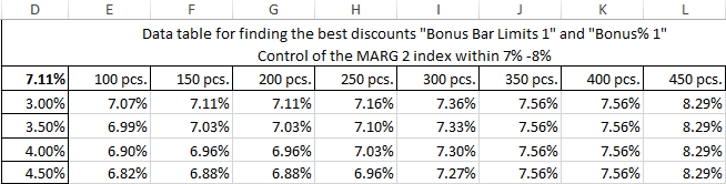
For finding to the optimal value from which depends on the result of the calculation, you need to create a data table in Excel. For easy assimilation of information we give the specific example of the data table.
For major client you must make a good discount that can afford the enterprise itself. The size of the discount depends from the purchasing power of the customer. We create to the matrix of numbers for quick selection of the best combinations in terms of discounts.
Using the data table in Excel
The data table – is this simulator, which works on the principle: « and what if?» by the way of lookup values for showing all possible combinations. The simulator watches about the changing of the cell values and displays how these changes will affect to the ending result in terms of the model of the loyalty program. The data table in MS Excel allows you to quickly analyze a set of likely outcomes model. When you configure only 2 options, you can get hundreds of combinations of results and then to select to the best of them.
This tool has undeniable advantages: all results appear in the one table on one sheet.
Creating of the data table in Excel
For starters we need to build 2 models:
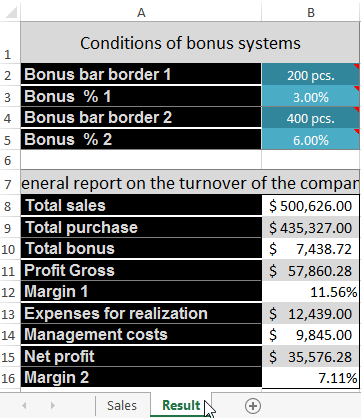
- The budget model company and the terms of the bonus system. To build such table you need to read the previous article: how to create a budget in Excel.
- The schema of the source data on the similarity of the «Table of Pythagoras». The string must contain a quantitative limit values for power-UPS, for example, all numbers from 100 to 500 in multiples of 50, and interest bonuses ranging from 3.0% to 10.0% of a multiple of 0.5%.
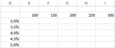
Attention! The cell (in this case D2) of the intersection of the row and column with filled values must be empty: as in the figure.
Now in the cell D2 we enter the formula is the same as for the calculation of the indicator «Margin 2»: = B15/B8 (the number format of cell is %).
Then we allocate to the range of cells D2:M17. Now for creating to the table data, you should choose to the «DATA», the section tools «Data Tools», tool «What-if Analysis» and option «Data Table».
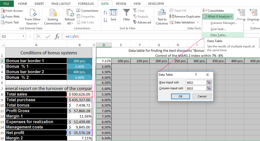
The dialog box «Data Table» will appear on the input parameters:
- The top field we fill by the absolute reference to the cell with a boundary strip of bonuses number $B$2.
- In the bottom field we refer to the value of the cell boundaries of percentage bonuses $B$3.
Attention! We expect to the optimal discounts for quantity 1 at current rates of boundary 2. For calculating discounts of quantitative discount border 2 in the boundary settings you should to show to the references on $B$4 and $B$5 are respectively.
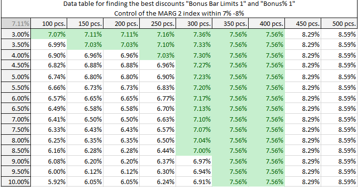
Click OK and the entire table is populated with the performance indicators «Margin 2» under appropriate conditions of bonus systems. In front of us once 135 options (all options should set to the format of cells in %).
The analysis what if in Excel data table
For the analysis using the data visualization we add to the conditional formatting:
- We allocate to the obtained results, and this is the cell range E3:M17.
- Choose to the tool: «HOME»-«Conditional Formatting»-«Highlight Cells Rules»-«Between».
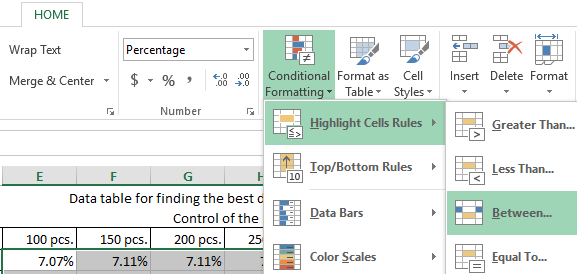
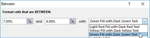
Specify to the borders from 7% to 8%, and specify to the desired format.
Now we can clearly see to the corridor for our profits, which we can’t go out for saving to the profit in certain limits. We can easily manage by the ratio of the quantity and discount and balance between the benefit for the customer and the seller. To do this, conditional formatting allows us to make a selection of data from the Excel table according to the criteria.
Thus, we have calculated to the optimal discounts for the border 1 with the current conditions of the border 2 and its bonus.
Bonus 2 and level for border 2 in the same way expect, only don’t forget to fill in the parameters correctly references $B$4 $B$5 are respectively.
The same way we can construct to the matrix for the indicator «NET Profit» and make for it to the desired conditional formatting. To mention profit with the conditional formatting we may in the range of 35 000 – 40 000.
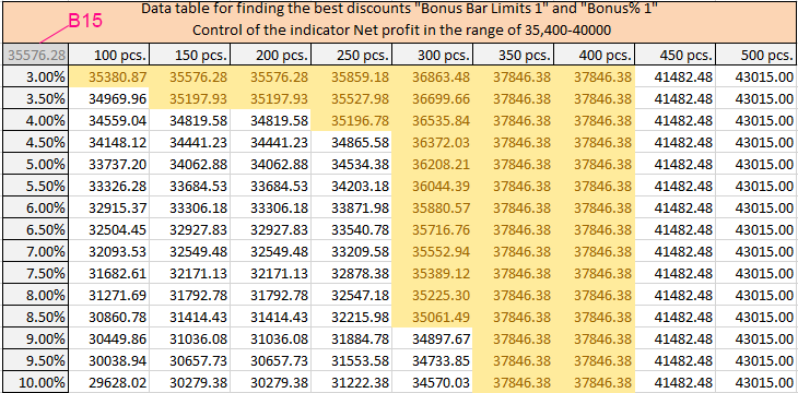
Now you can quickly and accurately to budget the best discounts that attract customers and do not bring the damage to the enterprise.
Download enterprise budget-bonus (the sample in Excel).
When negotiating with clients the question about loyalty is raised very often about bonuses and discounts. In such cases, you can quickly build a matrix for installing of multiple borders discounts under two conditions.
Read also the beginning of this article: Budgeting of the enterprise in Excel with discounts
This is the great tool from the point of view changes in two its parameters. It quickly provides a lot of important and useful information in a clear, simple and accessible form.