What is date format in excel - Word и Excel - помощь в работе с программами

Format numbers as dates or times

Excel for Microsoft 365 Excel for Microsoft 365 for Mac Excel for the web Excel 2021 Excel 2021 for Mac Excel 2019 Excel 2019 for Mac Excel 2016 Excel 2016 for Mac Excel 2013 Excel 2010 Excel 2007 Excel for Mac 2011 More…Less

When you type a date or time in a cell, it appears in a default date and time format. This default format is based on the regional date and time settings that are specified in Control Panel, and changes when you adjust those settings in Control Panel. You can display numbers in several other date and time formats, most of which are not affected by Control Panel settings.

Display numbers as dates or times

You can format dates and times as you type. For example, if you type 2/2 in a cell, Excel automatically interprets this as a date and displays 2-Feb in the cell. If this isn’t what you want—for example, if you would rather show February 2, 2009 or 2/2/09 in the cell—you can choose a different date format in the Format Cells dialog box, as explained in the following procedure. Similarly, if you type 9:30 a or 9:30 p in a cell, Excel will interpret this as a time and display 9:30 AM or 9:30 PM. Again, you can customize the way the time appears in the Format Cells dialog box.

On the Home tab, in the Number group, click the Dialog Box Launcher next to Number.

You can also press CTRL+1 to open the Format Cells dialog box.
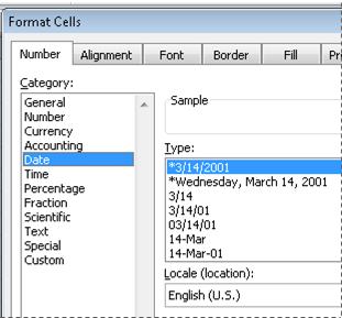
In the Category list, click Date or Time.
In the Type list, click the date or time format that you want to use.

Note: Date and time formats that begin with an asterisk (*) respond to changes in regional date and time settings that are specified in Control Panel. Formats without an asterisk are not affected by Control Panel settings.
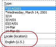
To display dates and times in the format of other languages, click the language setting that you want in the Locale (location) box.

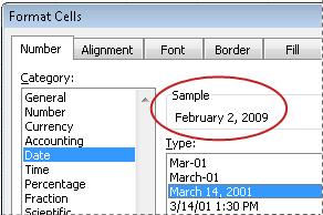
The number in the active cell of the selection on the worksheet appears in the Sample box so that you can preview the number formatting options that you selected.

Top of Page

Create a custom date or time format

On the Home tab, click the Dialog Box Launcher next to Number.

You can also press CTRL+1 to open the Format Cells dialog box.
In the Category box, click Date or Time, and then choose the number format that is closest in style to the one you want to create. (When creating custom number formats, it’s easier to start from an existing format than it is to start from scratch.)
In the Category box, click Custom. In the Type box, you should see the format code matching the date or time format you selected in the step 3. The built-in date or time format can’t be changed or deleted, so don’t worry about overwriting it.
In the Type box, make the necessary changes to the format. You can use any of the codes in the following tables:

Days, months, and years

To display	Use this code
Months as 1–12	m
Months as 01–12	mm
Months as Jan–Dec	mmm
Months as January–December	mmmm
Months as the first letter of the month	mmmmm
Days as 1–31	d
Days as 01–31	dd
Days as Sun–Sat	ddd
Days as Sunday–Saturday	dddd
Years as 00–99	yy
Years as 1900–9999	yyyy

If you use «m» immediately after the «h» or «hh» code or immediately before the «ss» code, Excel displays minutes instead of the month.

Hours, minutes, and seconds

To display	Use this code
Hours as 0–23	h
Hours as 00–23	hh
Minutes as 0–59	m
Minutes as 00–59	mm
Seconds as 0–59	s
Seconds as 00–59	ss
Hours as 4 AM	h AM/PM
Time as 4:36 PM	h:mm AM/PM
Time as 4:36:03 P	h:mm:ss A/P
Elapsed time in hours; for example, 25.02	[h]:mm
Elapsed time in minutes; for example, 63:46	[mm]:ss
Elapsed time in seconds	[ss]
Fractions of a second	h:mm:ss.00

AM and PM If the format contains an AM or PM, the hour is based on the 12-hour clock, where «AM» or «A» indicates times from midnight until noon and «PM» or «P» indicates times from noon until midnight. Otherwise, the hour is based on the 24-hour clock. The «m» or «mm» code must appear immediately after the «h» or «hh» code or immediately before the «ss» code; otherwise, Excel displays the month instead of minutes.

Creating custom number formats can be tricky if you haven’t done it before. For more information about how to create custom number formats, see Create or delete a custom number format.

Top of Page

Tips for displaying dates or times

To quickly use the default date or time format, click the cell that contains the date or time, and then press CTRL+SHIFT+# or CTRL+SHIFT+@.
If a cell displays ##### after you apply date or time formatting to it, the cell probably isn’t wide enough to display the data. To expand the column width, double-click the right boundary of the column containing the cells. This automatically resizes the column to fit the number. You can also drag the right boundary until the columns are the size you want.
When you try to undo a date or time format by selecting General in the Category list, Excel displays a number code. When you enter a date or time again, Excel displays the default date or time format. To enter a specific date or time format, such as January 2010, you can format it as text by selecting Text in the Category list.
To quickly enter the current date in your worksheet, select any empty cell, and then press CTRL+; (semicolon), and then press ENTER, if necessary. To insert a date that will update to the current date each time you reopen a worksheet or recalculate a formula, type =TODAY() in an empty cell, and then press ENTER.

Need more help?

You can always ask an expert in the Excel Tech Community or get support in the Answers community.

Need more help?

Want more options?

Explore subscription benefits, browse training courses, learn how to secure your device, and more.

Communities help you ask and answer questions, give feedback, and hear from experts with rich knowledge.

Источник

What is the Date Format in Excel?

In Excel, a date is displayed according to the format selected by the user. One can choose from the different formats available or create a customized format according to the requirement. The default date format is specified in the “Control Panel” of the system. However, it is possible to change these default settings.

For example, the date 01/01/2021 corresponds to the format dd/mm/yyyy. If the format is changed to d-mmm-yyyy, the date becomes 1-Jan-2021.

We can change the date format in Excel either from the “Number Format” of the “Home” tab or the “Format Cells” option of the context menu.

In Excel for Windows, 1900 is the default date system. Whereas, in Excel for Mac, 1904 is the default date system. Both these systems store the dates as consecutive numbers having a difference of 1. These numbers are known as serial values or serial numbers. The reason dates are stored as serial numbers is to facilitate calculations.

In the 1900 date system, the first date that Excel recognizes is January 1, 1900. This date is stored as the number 1 in Excel. Consequently, the number 2 represents January 2, 1900. The last date recognized by Excel is December 31, 9999. It is represented by the serial number 2958465. Date before 1900 or after 9999 is identified as a text value by Excel.

Dates are stored only as positive integers in the 1900 date system. However, to display negative numbers as negative dates, one needs to switch to the 1904 date system.

In the 1904 date system, 0 represents January 1, 1904, and -1 means January -2, 1904. The number 1 represents January 2, 1904. The last date recognized by Excel (in the 1904 date system) is December 31, 9999, represented by the serial number 2957003.

In this article, we follow the 1900 date system.

What is theDate Format in Excel?
- Code of Date Format in Excel
- How to Change Date Format in Excel?
  - Example #1–Apply Default Format of Long Date in Excel
  - Example #2–Change the Date Excel Format Using “Custom” Option
  - Example #3–Apply Different Types of Customized Date Formats in Excel
  - Example #4–Convert Text Values Representing Dates to Actual Dates
  - Example #5–Change the Date Format Using “Find and Replace” Box
- Frequently Asked Questions
- Recommended Articles

Code of Date Format in Excel

A code (like dd-mm-yyyy) is a representation of a day (d), month (m), and year (y). We can change the appearance of the date by changing the specified code.

The different codes, their explanation, and output (for days, months, and years) have been presented in the following images.

Notations for a Day

Notations for a Month

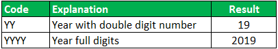
Notations for a Year

How to Change Date Format in Excel?

Here we look at some of the date format examples in Excel and how to change them.

Example #1–Apply Default Format of Long Date in Excel

The following image shows a number in cell A1. We want to know the date represented by this number. The output should be in the long date format of Excel.

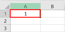
The steps to know the date represented by the number in cell A1 are listed as follows:

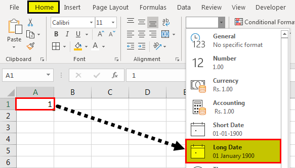
We must first select cell A1. Then, from the “Home” tab, click the “Number Format” drop-down appearing in the “Number” section. Next, select “Long Date,” shown in the following image.
The output is shown in the following image. The long date format displayed is dd mmmm yyyy. Hence, the number 1 represents the date 01 January 1900 in the long date format.
Note: The short and long dates appear as set in the “Control Panel.” Click “Clock, Language, and Region” in the “Control Panel” to change these default date formats. After that, click “Change date, time, or number formats.” Make the desired changes and click “OK.”

Likewise, had there been 2 in cell A1, the long date format would have been 02 January 1900. The number 3 would have been displayed as 03 January 1900 in the long date format.

Note: To switch to the 1904 date system, we must select “Advanced” from the “Options” of the “File” tab. Under “When calculating this workbook,” select “use 1904 date system” and click “OK.”

You can download this Change Date Format Excel Template here – Change Date Format Excel Template

Example #2–Change the Date Excel Format Using “Custom” Option

The following image shows some dates in the range A1:A6. These dates are in the format dd-mm-yyyy. We want to change their format to dd-mmmm-yyyy.

For instance, the date in cell A1 should appear as 25-February-2018. We may use the “Custom” option of the “Format Cells” dialog box.

The steps to change the date format in Excel are listed as follows:

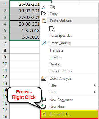
Step 1: We need to select all the dates of the range A1:A6. The same is shown in the following image.

Step 2: We must right-click the selection and choose “Format Cells” from the context menu. Alternatively, we may also press the keys “Ctrl+1” together.

Step 3: The “Format Cells” window opens, as shown in the following image.

Note: The default short date and long date formats are marked with an asterisk (*) in the box under “type.” The short date is 3/14/2012 (m/dd/yyyy), and the long date is Wednesday, March 14, 2012 (dddd, mmmm dd, yyyy).

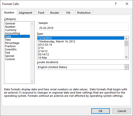
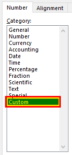
Step 4: From the “Number” tab, we need to select “Custom” under “Category.” The categories are shown on the left side of the “Format Cells” window.

Step 5: Under “Type,” we must insert the required date format. Either type the format (dd-mmmm-yyyy) or select it from the various options displayed in the box below “Type.”

Once the format has been entered, check the preview of the first date (of the range A1:A6) under “Sample.” The same is shown in the following image. Click “OK” in the “Format Cells” window if the date preview looks good.

Note 1: The date under “Sample” is displayed according to the format specified under “Type.”

Note 2: While creating custom date formats, we can use a forward slash (/), hyphen (-), comma (,), space ( ), etc.

Step 6: The output is shown in the following image. All dates of the range A1:A6 have been converted to the format dd-mmmm-yyyy. However, the Excel formula bar can still see the default date format. This default format corresponds with the short date set in the “Control Panel.”

Example #3–Apply Different Types of Customized Date Formats in Excel

The next image shows certain dates in the range A1:A6. At present, the date format is dd-mm-yyyy.

We want to apply four different formats to these dates. For using each format, the common steps to be performed are given as follows:

First, we must select the range A1:A6.
Then, right-click the selection and choose “Format Cells.”
After that, from the “Number” tab, select “Custom” under “Category.”

Further, under each format, the additional steps to be performed followed by two images are given.

Format 1: dd-mmm-yyyy

In the “Custom” option of the “Number” tab, select the format “dd-mmm-yyyy” under “Type.”
Click “Ok.”

The output is given in the following image. All dates are displayed according to the format dd-mmm-yyyy. The hyphen is the separator between the day, month, and year in this format.

Format 2: dd mmm yyyy

We must select the format “dd mmm yyyy” under “Type” of the “custom” option.
Click “Ok.”

The output is given in the following image. All dates are converted to the format dd mmm yyyy. The space is the only separator between the day, month, and year in this format.

Format 3: ddd mmm yyyy

In the “Custom” option, select the format “ddd mmm yyyy” under “Type.”
Click “Ok.”

The output is given in the following image. The dates are shown in the format ddd mmm yyyy. The day and the month are displayed in their short notations in this format.

Format 4: dddd mmmm yyyy

From the “Custom” option of the “Number” tab, select “dddd mmmm yyyy” under “Type.”
Click “Ok.”

The output is given in the following image. All dates have been converted to the format dddd mmmm yyyy. The date, month, and year are displayed in their respective full forms in this format.

It must be observed that the date format changes as per the style set by the user. Therefore, the user can select a date format according to their convenience.

Example #4–Convert Text Values Representing Dates to Actual Dates

The following image shows a list of dates in the range A1:A6. At present, these dates are appearing as text values. We want to convert these text values to dates having the format dd-mmm-yyyy.

The steps to convert text values to dates having the given format are listed as follows:

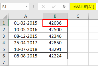
Step 1: First, enter the following formula in cell B1.

“=VALUE(A1)”

Then, press the “Enter” key.

Note 1: The VALUE functionIn Excel, the value function returns the value of a text representing a number. So, if we have a text with the value $5, we can use the value formula to get 5 as a result, so this function gives us the numerical value represented by a text.read more returns the numeric form of a text string that represents a number. In other words, it converts a number looking like the text into an actual number.

Note 2: Instead of the VALUE function, one can also use the DATEVALUE functionThe DATEVALUE function in Excel shows any given date in absolute format. This function takes an argument in the form of date text normally not represented by Excel as a date and converts it into a format that Excel can recognize as a date.read more of Excel. The latter converts a date stored as text to a serial number. This serial number is recognized as a date by Excel.

Step 2: We must select cell B1 and drag the fill handle until cell B6. The output is shown in the following image. All text values (A1:A6) have been converted to numbers (in the range B1:B6).

Ideally, the text string in Excel is left-aligned while the number string is right-aligned. However, we have centrally aligned both the ranges (A1:A6 and B1:B6).

Note: When text strings representing dates have been converted to serial values (or dates), we can use them for performing different calculations like addition, subtraction, and so on.

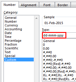
Step 3: To view the obtained serial numbers (in column B) as dates, apply the required format. We must select the range B1:B6, right-click and choose “Format Cells.”

In the “Number” tab, select the option “Custom.” Then, under “Type,” enter or choose the format “dd-mmm-yyyy.” The same is shown in the following image.

If the sample date looks alright, click “OK.”

Step 4: The output is shown in the following image. Hence, all text values (of column A) have been converted to valid dates (in column B) having the format dd-mmm-yyyy.

Note: To ensure that a value is recognized as a date by Excel, check for the following signs:

The dates are right-aligned as they are numerical values.
If two or more dates are selected, the status bar (at the bottom of the worksheet) shows the count, average, numerical count, and sum. In addition, it may display one or more options according to the Excel version.

If a value is a text string, it would be left-aligned, and the status bar will show only the count.

Often, the Excel date format needs to be changed (from text to dates) when data is downloaded (or copied and pasted) from the web. That is because, in such instances, the dates may not be displayed as numbers.

Example #5–Change the Date Format Using “Find and Replace” Box

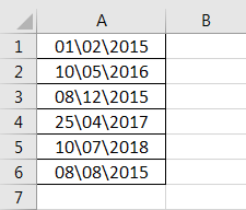
The following image shows some text values representing dates in the range A1:A6. The days, months, and numbers have been separated with a backslash. That is because we want to perform the following tasks:

Replace all the backslashes () with forwarding slashes (/) by using the “Find and Replace” dialog box.
Convert text values representing dates to actual dates.

The steps to perform the given tasks are listed as follows:

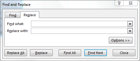
Step 1: We must press the keys “Ctrl+H” together. Then, the “find and replace” dialog box opens, as shown in the following image.

Step 2: Type a backslash in the “Find what” box (). In the “Replace with” box, type a forward slash (/).

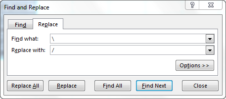
Step 3: Next, we must click “Replace All.” Excel shows a message stating the number of replacements it has made. Click “OK” to proceed. The final output is shown in the following image.

Hence, all backslashes have been replaced with forwarding slashes. With this replacement, the text values representing dates have automatically been converted to actual dates by Excel.

Since column A was aligned centrally from the beginning, this alignment is retained even after the values are converted to dates.

Frequently Asked Questions

1. How can the date format in Excel be changed?

The steps to change the date format in Excel are listed as follows:
The steps to change the date format in Excel are listed as follows:

a. Select the cell containing the date. If the date format of a range needs to be changed, select the entire range.
b. Right-click the selection and choose “Format Cells” from the context menu. Alternatively, press the keys “Ctrl+1” together.
c. IIn the “Number” tab, select the option “Date.” Next, select the required date format under “Type.”
d. Check the preview (of the first date of the selected range) under “Sample.” If the preview is good, click “OK.”

The date format of the selected cell or cells (selected in step a) is changed.

Note 1: The required date format may not be available under the “Date” option’s “Type.” If it is not available, select “Custom” as the “category” from the “Number” tab. Then, type the required date format under “Type” and click “OK.”

Note 2: If the selected cell (selected in step a) contains a text string representing a date, convert this string to date first. Then change the format to the desired date format.

2. How to change the date format permanently in Excel?

To change a date format permanently, one needs to make changes to the date formats of the “Control Panel.” That is because the short and long date formats of Excel reflect the date settings of the “Control Panel.”

The steps to change the date settings of the “Control Panel” are listed as follows:

We must open the “Control Panel” first from the “Start” menu.
b. In the “Clock, Language, and Region” category, click “Change date, time, or number format.” It is available under the “Region and Language” option.
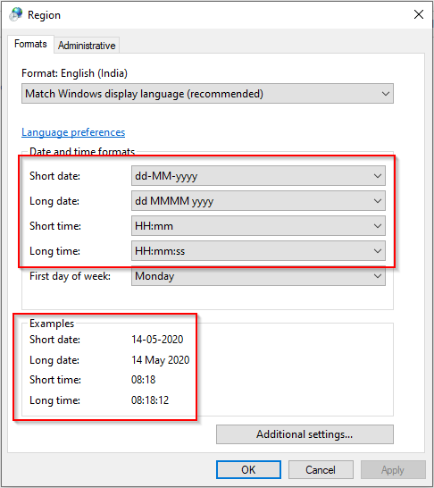
c. The “Region and Language” or “Region” dialog box opens. Under “Format,” we must select the region.
d. Enter the required short and long date formats under “Date and Time Formats.” To enter customized short and long date formats, click “Additional Settings.” The “Customize Format” dialog box opens. Make the changes in the “Date” tab and click “OK.”
e. Check the preview under “Examples” at the bottom of the “Region and Language” box. If the preview is alright, click “OK.”

The default date settings have been changed. Now, we should enter a date in any format in Excel. Then select the short or the long date format from the “Number Format” (in the “Number” section) of the “Home” tab.
The dates will appear in the format set in the “Control Panel.” So, the user need not change the format of each date manually.

3. How to change a date to a text string in Excel?

Let us change the date 22/1/2019 in cell A1 to a text string in Excel. The text string should be in the format yyyy-mm-dd.

The steps to change a date to a text string are listed as follows:
a. First, we must enter the formula =TEXT(A1, “yyyy-mm-dd”) in cell B1.
b. Then, press the “Enter” key.

The date in cell A1 (22/1/2019) is converted to 2019-01-22 in cell B1. We must note that the date in cell A1 is right-aligned, being a number. In contrast, the text in cell B1 is left-aligned.

Note: The TEXT function helps convert numbers to text strings. It is used to display values in a specific format. The syntax is TEXT(value,format_text). “Value” is the number to be converted to text. “Format_text” is the format in which the number should be displayed.

What is a date in Excel?

A date is a number! And like any number (currency, percentage, decimal, …), you can customize your date format 👍

Dates are whole numbers

Usually, when you insert a date in a cell it is displayed in the format dd/mm/yyyy or mm/dd/yyyy.

Let’s say you have the date 01/01/2016 in a cell. If you change the cell’s format to Standard, the cell displays 42370 😕🤔

Explanation of the numbering

In Excel, a date is the number of days since 01/01/1900 (the first date in Excel).

So 42370 is the number of days between 01/01/1900 and 01/01/2016.

Date format

Dates can be displayed in different ways using the following 2 options (available in the Number Format dropdown in the main menu):

Short Date
Long Date

How to customize a date?

To customize a date:

Open the dialog box Custom Number (with the shortcut Ctrl + 1 or by clicking on the menu More number formats at the bottom of the number format dropdown)

In this dialog box, you select ‘Custom‘ in the Category list and write the date format code in ‘Type‘.

To format a date, you just write the parameter d, m or y a different number of times. For example,

dd/mm/yyyy will display 01/01/2016
dd mmm yyyy => 01 Jan 2016
mmmm yyyy => January 2016
dddd dd => Friday 01

In function of your language , the letter could be different:

t for «tag» (day) in German
j for «jour» (day) in French
a for «año» (year) in Spanish

Don’t write text in your cell !!!

With dates, one of the most common mistakes is to write text inside the format code (1 January 2016 for example). Never do this in Excel ⛔⛔⛔

If you do this, the contents of the cell will be Text and not a number

In Excel, text is always displayed on the left of a cell.
A number or a date is displayed on the right.

If you want to display the month in letters, just change the month format of your date.

Different examples of custom date

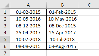
The following document shows you the same date but in different formats. The code for each date is in column A.

Different writing of dates according to the format code

In the following document, you can see the impact of each format on the same date.

Источник

I am sure that every excel user like you 😉 frequently work with dates and times in excel. Some may follow the excel date format in DD-MM-YYYY (like in India) and others may follow MM-DD-YYYY (like in US). Similarly, the time may be in HH:MM or HH:MM:SS format in excel.

But do you know how excel understands and interprets the dates and times in the backend? Probably your answer is NO!

Table of Contents

Basics of Date and Time Format in Excel
Behind the Scenes 😉 – Excel Date
Behind the Scenes 😉 – Excel Time
2 Methods to Find Number Value of Date and Time
1. Method 1 # Change Cell Format to General
2. Method 2 # Using Excel DATEVALUE and TIMEVALUE Excel Function

No worries 😎 In this tutorial, we would learn everything about what excel does behind the scenes while you enter any date and time in the excel cell.

Here we go 😎

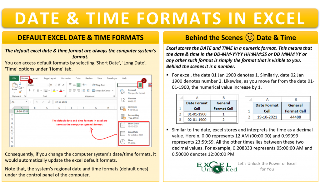
The default excel date and time format are always the computer system’s format.

You can access the default formats by selecting the ‘Short Date’, ‘Long Date’, ‘Time’ options under ‘Home’ tab, as shown below:

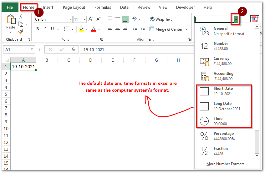
The above formats (DD-MM-YYYY, DD MMMM YYYY, and HH:MM:SS) correspond to the computer system’s regional formats under the control panel.

Consequently, if you change the computer system’s date/time formats, it would automatically update the excel default formats.

Let us learn how excel reads and interprets the date or time that you enter the cell.

Behind the Scenes 😉 – Excel Date

As soon as you enter any date (any format) in an excel cell, the excel stores that date as a numerical number.

This means that the date in the DD-MM-YYYY or DD MMM YY or any other such format is simply visible to you. Behind the scenes, Excel understands and stores it in the form of some numerical value. But, what is this numerical value of date? Read below text.

To understand this, let us do a very simple exercise. Open a new excel workbook and type the date 01-01-1900 in any of the cells and press Enter. Now, select this cell and change the cell format to ‘General’.

As a result, you would notice that the excel returns 1 as output.

Do you know why did this happen? The simple answer to this is that for excel, the date 01-01-1900 is 1.

Now, change the date to 02-01-1900 and cell format to ‘General’. The result is 2. It means excel interprets date 02-01-1900 as 2.

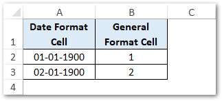
Likewise, as you move far from the date 01-01-1900, the numerical value increase by 1.

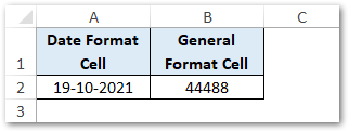
Therefore, the numerical value of the date 19-10-2021 is 44488. This simply denotes, the date 19-10-1996 is 44488 days away from 01-01-1900.

Behind the Scenes 😉 – Excel Time

Similar to the date, excel stores and interprets the time as a decimal value. Herein, 0.00 represents 12 AM (00:00:00) and 0.99999 represents 23:59:59.

All the other times lies between these two decimal values. For example, 0.208333 represents 05:00:00 AM and 0.50000 denotes 12:00:00 PM.

2 Methods to Find Number Value of Date and Time

There are two methods for finding the number value of date and time in excel:

Changing Cell Format to ‘General’ (without formula)
Using DATEVALUE and TIMEVALUE excel formula

Method 1 # Change Cell Format to General

If you have a date in a cell and you want to find the numerical value of that date without using formula, follow these steps:

Select cell(s) containing date (say date is 01-04-2020)

Navigate to the ‘Home’ tab > ‘Number’ group. Click on the drop down button and select the format as ‘General’

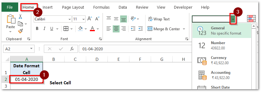
As a result, excel returns the number value of the date as 43922.

Likewise, it works the same in the case of time.

Method 2 # Using Excel DATEVALUE and TIMEVALUE Excel Function

Excel has come up with a separate formula to convert the date or time into the corresponding date and time number format.

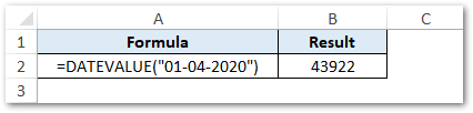
Simply pass the date within double-quotes as function argument.

=DATEVALUE("01-04-2020")

As a result, excel returns the number value, as shown below:

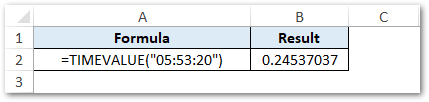
The same goes with the TIMEVALUE function:

=TIMEVALUE(“05:53:20”)

Every other excel date and time formula (like EDATE, EOMONTH, etc.) uses the date/time numerical value to perform arithmetical calculations on it.

Thank you for reading 🙂

Excel TEXT Function – Convert Number In Text Format
TIME Function in Excel – Returning The Time Format
How to Convert Time into Decimal Number, Hours, Minutes or Seconds
DATE Function in Excel – Get Date Using Excel Formula
TIMEVALUE Function in Excel – Returning Serial Number of Time
DATEVALUE function in Excel – Get Date Serial Number

Источник

m/d/yyyy.
Click Home tab, then click the drop-down menu in Number Format Tools. Step 2. Select Short Date from the drop-down list. The date is instantly displayed in short date format m/d/yyyy.

Contents

1 What is the standard date format in Excel?
2 What date format is mm dd yyyy?
3 What is the date format?
4 How do you format a date in Excel?
5 What is the short date today?
6 How do you format a date in dd-mm-yyyy in Excel?
7 How do you format YYYY?
8 How do you write the date format?
9 How do you format the date?
10 How do I format a full date?
11 Why is my date not formatting in Excel?
12 What is the date value in Excel?
13 How do I convert a date in Excel to date format?
14 Why is April called April?
15 How many days is 2021 so far?
16 Is July the 7th month?
17 What does YYYY format mean?
18 How do you do mm dd yyyy?
19 How do I format mm yyyy in Excel?
20 How do you write day date and time?

The default date system for Excel for Windows is 1900; and the default date system for Excel for Mac is 1904.

What date format is mm dd yyyy?

Date/Time Formats

Format	Description
MM/DD/YY	Two-digit month, separator, two-digit day, separator, last two digits of year (example: 12/15/99)
YYYY/MM/DD	Four-digit year, separator, two-digit month, separator, two-digit day (example: 1999/12/15)

What is the date format?

Date Format Types

Format	Date order	Description
1	MM/DD/YY	Month-Day-Year with leading zeros (02/17/2009)
2	DD/MM/YY	Day-Month-Year with leading zeros (17/02/2009)
3	YY/MM/DD	Year-Month-Day with leading zeros (2009/02/17)
4	Month D, Yr	Month name-Day-Year with no leading zeros (February 17, 2009)

How do you format a date in Excel?

In an Excel sheet, select the cells you want to format. Press Ctrl+1 to open the Format Cells dialog. On the Number tab, select Custom from the Category list and type the date format you want in the Type box. Click OK to save the changes.

What is the short date today?

Today’s Date

Today’s Date in Other Date Formats
Unix Epoch:	1639448931
RFC 2822:	Mon, 13 Dec 2021 18:28:51 -0800
DD-MM-YYYY:	13-12-2021
MM-DD-YYYY:	12-13-2021

How do you format a date in dd-mm-yyyy in Excel?

You have to create a custom date format for your requirement as it does not exist in excel by default. First select your cells containing dates and right click of mouse and select Format Cells. In Number Tab, select Custom then type ‘dd-mmm-yyyy’ in Type text box, then click okay. It will format your selected dates.

How do you format YYYY?

The correct format of your date of birth should be in dd/mm/yyyy. For example, if your date of birth is 9th October 1984, then it will be mentioned as 09/10/1984.

How do you write the date format?

The international standard recommends writing the date as year, then month, then the day: YYYY-MM-DD. So if both the Australian and American used this, they would both write the date as 2019-02-03. Writing the date this way avoids confusion by placing the year first.

How do you format the date?

Follow these steps:

Select the cells you want to format.
Press CTRL+1.
In the Format Cells box, click the Number tab.
In the Category list, click Date.
Under Type, pick a date format.
If you want to use a date format according to how another language displays dates, choose the language in Locale (location).

How do I format a full date?

The United States is one of the few countries that use “mm-dd-yyyy” as their date format–which is very very unique! The day is written first and the year last in most countries (dd-mm-yyyy) and some nations, such as Iran, Korea, and China, write the year first and the day last (yyyy-mm-dd).

Why is my date not formatting in Excel?

If you want to sort the dates, or change their format, you’ll have to convert them to numbers – that’s how Excel stores valid dates. Sometimes, you can fix the dates by copying a blank cell, then selecting the date cells, and using Paste Special > Add to change them to real dates.

What is the date value in Excel?

The Excel DATEVALUE function converts a date represented as a text string into a valid Excel date. For example, the formula =DATEVALUE(“3/10/1975”) returns a serial number (27463) in the Excel date system that represents March 10, 1975.

How do I convert a date in Excel to date format?

How to change text to date in Excel an easy way

Select the cells with text strings and click the Text to Date button.
Specify the date order (days, months and years) in the selected cells.
Choose whether to include or not include time in the converted dates.
Click Convert.

Why is April called April?

APRIL: The name for this month may come from a Roman word for “second” – aprilis – as it was the second month of the Roman year. MAY: Spring is in full bloom for the Romans in May, and this month is named after Maia – a goddess of growing plants.

How many days is 2021 so far?

The year 2021 has 365 days. Today (day 346, Sunday, December 12th) is highlighted. ‘Percent of year’ shows the percentage the year is complete at midnight (start of the day). Week number according to ISO-8601.

Is July the 7th month?

July, seventh month of the Gregorian calendar. It was named after Julius Caesar in 44 bce. Its original name was Quintilis, Latin for the “fifth month,” indicating its position in the early Roman calendar.

What does YYYY format mean?

Filters. Abbreviation for the four-digit display of a year, as in 2007. 16.

How do you do mm dd yyyy?

Write dates like YYYY-MM-DD

Select the column.
In the menu bar, select Format → Cells.
Choose “Text” on the left.

How do I format mm yyyy in Excel?

On the cell you wish to format, right click -> Format cells, click on “Custom” under Category tab, type in “mm/yyyy” below the “Type” textbox, click on OK. Where is the problem? The date is in the format dd/mm/yyyy.

How do you write day date and time?

In traditional American usage, dates are written in the month–day–year order (e.g. December 13, 2021) with a comma before and after the year if it is not at the end of a sentence, and time in 12-hour notation (2:05 am).

Источник

In this article

Display numbers as dates or times

Create a custom date or time format

Tips for displaying dates or times

Need more help?

Need more help?

Want more options?

What is the Date Format in Excel?

Table of contents

Code of Date Format in Excel

How to Change Date Format in Excel?

Example #1–Apply Default Format of Long Date in Excel

Example #2–Change the Date Excel Format Using “Custom” Option

Example #3–Apply Different Types of Customized Date Formats in Excel

Example #4–Convert Text Values Representing Dates to Actual Dates

Example #5–Change the Date Format Using “Find and Replace” Box

Frequently Asked Questions

Recommended Articles

What is a date in Excel?

Dates are whole numbers

Explanation of the numbering

Date format

How to customize a date?

Don’t write text in your cell !!!

Different examples of custom date

Different writing of dates according to the format code

Behind the Scenes 😉 – Excel Date

Behind the Scenes 😉 – Excel Time

2 Methods to Find Number Value of Date and Time

Method 1 # Change Cell Format to General

Method 2 # Using Excel DATEVALUE and TIMEVALUE Excel Function

RELATED POSTS

What date format is mm dd yyyy?

What is the date format?

How do you format a date in Excel?

What is the short date today?

How do you format a date in dd-mm-yyyy in Excel?

How do you format YYYY?

How do you write the date format?

How do you format the date?

How do I format a full date?

Why is my date not formatting in Excel?

What is the date value in Excel?

How do I convert a date in Excel to date format?

Why is April called April?

How many days is 2021 so far?

Is July the 7th month?

What does YYYY format mean?

How do you do mm dd yyyy?

How do I format mm yyyy in Excel?

How do you write day date and time?