
Date and time in excel are treated a bit differently in excel than in other spreadsheets software. If you don’t know how Excel date and time work, you may face unnecessary errors.
So, in this article, we will learn everything about the date and time of Excel. We will learn, what are dates in excel, how to add time in excel, how to format date and time in excel, what are date and time functions in excel, how to do date and time calculations (adding, subtracting, multiplying etc. with dates and times).
What is Date and Time in Excel?
Many of you may already know that Excel dates and time are nothing but serial numbers. A date is a whole number and time is a fractional number. Dates in excel have different regional formatting. For example, in my system, it is mm/dd/YYYY (we will use this format throughout the article). You may be using the same date format or you could be using dd/mm/YYYY date format.
Date Formatting of Cell
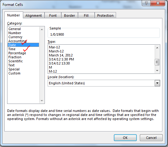
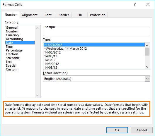
There are multiple options available to format a date in Excel. Select a cell that may contain a date and press CTRL+1. This will open the Format Cells dialogue box. Here you can see two formatting options as Date and Time. In these categories, there are multiple date formattings available to suit your requirements.
 Dates:
Dates in Excel are mare serial numbers starting from 1-Jan-1900. A day in excel is equal to 1. Hence 1-Jan-1900 is 1, 2-Jan-1900 is 2, and 1-Jan-2000 is 36526.
Fun Fact: 1900 was not a leap year but excel accepts 29-Feb-1900 as a valid date. It was a desperate glitch to compete Lotus 1-2-3 back in those days.
Shortcut to enter static today’s date in excel is CTRL+; (Semicolon).
To add or subtract a day from a date you just need to subtract or add that number of days to that date.
Time:
Excel by default follows the hh:mm format for time (0 to 23 format). The hours and minutes are separated by a colon without any spaces in between. You can change it to hh:mm AM/PM format. The AM/PM must have 1 space from the time value. To include seconds, you can add :ss to hh:mm (hh:mm:ss). Any other time format is invalid.
Time is always associated with a date. The date comes before the time value separated with a space from time. If you don’t mention a date before time, by default it takes the first date of excel (which is 1/1/1900). Time in excel is a fractional number. It is shown on the right side of the decimal.
Hours:
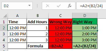
Since 1 day is equal to 1 in excel and 1 day consists of 24 hours, 1 hour is equal to 1/24 in excel. What does that mean? It means that if you want to add or subtract 1 hour to time, you need to add or subtract 1/24. See the image below.
 you can say that 1 hour is equal to 0.041666667 (1/24).
Calculate hours between time in Excel
Minutes:
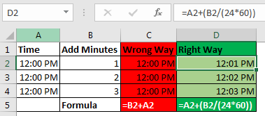
From the explanation of the hour in excel, you must have guessed that 1 Minute in excel is equal to 1/(24×60) (or 1/1440 or 0.000694444).
If you want to add a minute to an excel time, add 1/(24×60). See the image below. Sometimes you get the need to Calculate Minutes Between Dates & Time In Excel, you can read it here.
 Seconds:
Yes, a second in Excel is equal to 1/(24x60x60). To add or subtract seconds from a time, you just need to do the same things as we did in minutes and hours.
Date and Time in one cell
Dates and times are linked together. A date is always associated with a valid date and time is always associated with a valid excel date. Even if you are not able to see one of them.
If you only enter a time in a cell, the date of that cell will 1-Jan-1900, even if you are not able to see it. If you format that cell as a date-time format, you can see the associated date. Similarly, if you don’t mention time with the date, by default 12:00 AM is attached. See the image below.
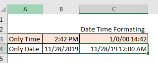
In the image above, we have time only in B3 and date only in B4. When we format these cells as mm/dd/yy hh:mm, we get both, time and date in both cells.
So, while doing date and time calculations in excel, keep this in check.
No Negative Time
As I told you the date and time in excel starts from 1-Jan-1900 12:00 AM. Any time before this is not a valid date in excel. If you subtract a value from a date that leads to before 1-Jan-1900 12:00, even one second, excel will produce ###### error. I have talked about it here and in Convert Date and Time from GMT to CST. It happens when we try to subtract something that leads to before 1 Jan-1900 12:00. Try it yourself. Write 12:00 PM and subtract 13 hours from it. see what you get.
Calculations with Dates and Time in Excel
Adding Days to a date:
Adding days to a date in excel is easy. To add a day to date just add 1 to it. See the image below.
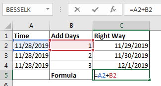
You should not add two dates to get the future date, as it will sum up the serial numbers of those days and you may get a date far in the future.
Subtracting Days from Date:
If you want to get a backdate from a date a few days before, then just subtract that number of days from the date and you will get backdate. For example, if I want to know what date was before 56 days since TODAY then I would write this formula in the cell.
This will return us the date of 56 before the current date.
Note: Remember that you can not have a date before 1/Jan/1900 in excel. If you get ###### error, this could be the reason.
Days between two dates:
To calculate days between two dates we just need to subtract the start date from the end date. I have already done an article on this topic. Go and check it out here. You can also use the Excel DAYS Function to calculate days between a start date and end date.
Adding Times:
There’s been a lot of queries on how to add time to excel as many people get confusing results when they do it. There are two types of addition in times. One is adding time to another time. In this case, both times are formatted as hh:mm time format. In this case, you can simply add these times.
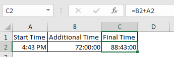
The second case is when you don’t have additional time in time format. You just have numbers of hours, minutes and seconds to add. In that case, you need to convert those numbers to their time equivalents. Note these points to add hours, minutes and seconds to a date/time.
- To add N hours to an X time use formula =X+(N/24) (As 1=24 hours)
- To Add N minutes to X time use formula = X+(N/(24*60))
- To Add N Second to X time use formula = X+(N/(24*60*60))
Subtracting Times
It’s the same as adding time, just make sure that you don’t end up with a negative time value when subtracting, because there is no such thing as a negative number in excel.
Note: When you add or subtract time in excel that exceeds 24 hours of difference, excel will roll to the next or previous date. For example, if you subtract 2 hours from 29-Jan-2019 1:00 AM then it will roll back to 28-Jan-2019 11:00 PM. If you subtract 2 hours from 1:00 AM (does not have the date mentioned), Excel will return ###### error. I have told the reason at the beginning of the article.
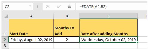
Adding Months to a Date:
You can’t just add multiples of 30 to add months to date as different months have a different number of days. You need to be careful while adding months to Date. To add months to a date in excel, we use EDATE function of excel. Here I have a separate article on adding months to a date in different scenarios.
 Adding years to date:
Just like adding months to a date, it is not straightforward to add years to date. We need to use YEAR, MONTH, DAY function to add years to date. You can read about adding years to date here.
If you want to calculate years between dates then you can use this.
Excel Date and Time Handling Functions:
Since date and time are special in Excel, Excel provides special functions to handle them. Here I am mentioning a few of them.
- TODAY(): This function returns today’s date dynamically.
- DAY(): Returns Day of the month (returns number 1 to 31).
- DAYS(): Used to count the number of days between two dates.
- MONTH(): Used to get the month of the date (returns number 1 to 12).
- YEAR(): Returns year of the date.
- WEEKNUM(): Returns the weekly number of a date, in a year.
- WEEKDAY(): Returns the day number in a week (1 to 7) of the supplied date.
- WORKDAY(): Used to calculate working days.
- TIMEVALUE(): Used to extract Time value (serial number) from a text formatted date and time.
- DATEVALUE(): Used to extract date value (serial number) from a text formatted date and time.
These are some of the most useful data and time functions in excel. There are plenty more date and time functions. You can check them out here.
Date and Time Calculations
If I explain all of them here, this article will get too long. I have divided these time calculation techniques in excel into separate articles. Here I am mentioning them. You can click on them to read.
- Calculate days, months and years
- Calculate age from date of birth
- Multiplying time values and numbers.
- Get Month name from Date in Excel
- Get day name from Date in Excel
- How to get a quarter of the year from date
- How to Add Business Days in Excel
- Insert Date Time Stamp with VBA
So yeah guys, this is all about the date and time in excel you need to know about. I hope this article was useful to you. If you have any queries or suggestions, write them down in the comments section below.
The objective of this post is to teach you how Excel handles date and time and provide you with all the tools you will need.
It’s designed to be read in conjunction with the accompanying Excel file, which you can download below.
Download the Files
Enter your email address below to download the comprehensive Excel workbook and PDF.
By submitting your email address you agree that we can email you our Excel newsletter.
Regional Settings
When reading this post keep in mind that my regional settings format dates as dd/mm/yyyy and so the screenshots throughout this post are in this format. However, if you open the accompanying Excel file you may see some dates have switched to match your regional settings, which may be different to mine e.g. mm/dd/yyyy.
Dates and times with a format that begins with an asterisk (*) automatically update based on your PC’s regional settings. You can see an example in the Format Cells dialog box below:
Ok, let’s crack on.
Excel Date and Time 101
Excel stores dates and time as a number known as the date serial number, or date-time serial number.
When you look at a date in Excel it’s actually a regular number that has been formatted to look like a date. If you change the cell format to ‘General’ you’ll see the underlying date serial number.
The integer portion of the date serial number represents the day, and the decimal portion is the time. Dates start from 1st January 1900 i.e. 1/1/1900 has a date serial number of 1.
Caution! Excel dates after 28th February 1900 are actually one day out. Excel behaves as though the date 29th February 1900 existed, which it didn’t.
Microsoft intentionally included this bug in Excel so that it would remain compatible with the spreadsheet program that had the majority market share at the time; Lotus 1-2-3.
Lotus 1-2-3 was incorrectly programmed as though 1900 was a leap year. This isn’t a problem as long as all your dates are later than 1st March 1900.
Excel gives each date a numeric value starting at 1st January 1900. 1st January 1900 has a numeric value of 1, the 2nd January 1900 has a numeric value of 2 and so on. These are called ‘date serial numbers’, and they enable us to do math calculations and use dates in formulas.
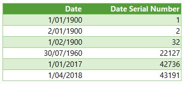
The Date Serial Number column displays the Date column values in their date serial number equivalent.
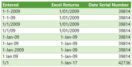
e.g. 1/1/2017 has a date serial number of 42736. i.e. 1st January 2017 is 42,736 days since 31st December 1899.
Tip: format the date serial number column as a Date and you’ll see they look the same as the Date column values.
Time
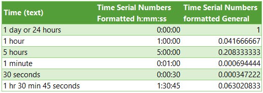
Times also use a serial number format and are represented as decimal fractions.
Hours: since 24 hours = 1 day, we can infer that 24 hours has a time serial number of 1, which can be formatted as time to display 24:00 or 12:00 AM or 0:00. Whereas 12 hours or the time 12:00 has a value of 0.50 because it is half of 24 hours or half of a day, and 1 hour is 0.41666′ because it’s 1/24 of a day.
Minutes: since 1 hour is 1/24 of a day, and 1 minute is 1/60 of an hour, we can also say that 1 minute is 1/1440 of a day, or its time serial number is 0.00069444′
Seconds: since a second is 1/60 of a minute, which is 1/60 of an hour, which is 1/24 of a day. We can also say one second is 1/86400 of a day or in time serial number form it’s 0.0000115740740740741…
Date & Time Together
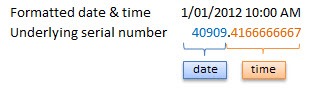
Now that we know how dates and times are stored we can put them together — ddddd.tttttt
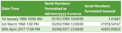
For example, the date and time of 1st January 2012 10:00:00 AM has a date-time serial value of 40909.4166666667
40909 being the serial value representing the date 1st January 2012, and .4166666667 being the decimal value for the time 10:00 AM and 00 seconds.
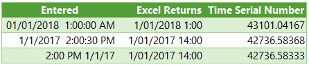
More examples below.
Entering Dates & Times in Excel
Entering Dates
You can type in various configurations of a date and Excel will automatically recognise it as a date and upon pressing ENTER it will convert it to a date serial number and apply a date format on the cell.
For example, try typing (or even copy and paste) the following dates into an empty cell:
| 1-1-2009 |
| 1-1-09 |
| 1/1/2009 |
| 1/1/09 |
| 1-Jan-09 |
| 1-Jan 09 |
| 1-Jan-2009 |
| 1 Jan 09 |
| 1/1 |
You can see in the table above that entering numbers that look like dates and are separated by a forward slash or hyphen will be recognised as a date. Even typing in a date with the month name gets converted to a date.
However, dates separated with a period like this 1.1.2009, or with spaces between numbers like this 01 01 2009, will end up as text, not a date. Gotta have some limits!
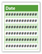
Tip: Dates that display ##### in a cell usually indicate that the column is simply not wide enough to display it.
However, if you make the cell really wide and it still displays ##### then this indicates that the date is a negative value and Excel can’t display negative dates.
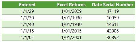
Entering Dates with Two Digit Years
When you enter a date with two digits for the year e.g. 1/1/09, Excel has to decide if you mean 2009 or 1909.
It goes by the rule that dates with years 29 or before, are treated as 20xx and dates with the year 30 or older are treated as 19xx. See examples below.
Tip: You can enter the day and month portions of a date and Excel will insert the year based on your computer’s clock. Nice to know for data entry.
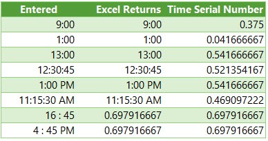
Entering Time
When you enter time you must follow a strict format of at least h:mm. i.e. the hour and minutes are separated by a colon with no spaces either side. Entering the h:mm components will result in a time formatted in military time e.g. 2:00 PM is 14:00 in military time.
If you enter a time that includes a seconds component e.g. 3:15:40, Excel will automatically format the cell in h:mm:ss.
If you want the time to be formatted with AM/PM you can simply enter a space after the time and then type AM or PM, or apply the number format to the cell later. Here are some examples:
Entering Dates & Time Together
Now that we know how to enter dates and time separately we can put them together to enter a date and time in the same cell.
You can even enter time then date and Excel will fix the order for you.
You’ll find that even if you enter AM/PM, that Excel will convert it to military time by default. You can override this with a custom number format. More on that later.
Simple Date & Time Math
Now that we understand that Excel stores dates and time as serial numbers, you’ll see how logical it is to perform math operations on these values. We’ll look at some simple examples here and tackle the more complex scenarios later when we look at Date and Time Functions.
Adding/Subtracting Days from Dates
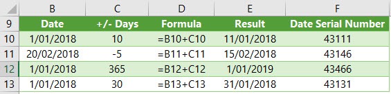
Tip: you can also add/subtract the days directly in the formula e.g. =B10+10 or =B11-5 Although, it’s better to place the values you’re adjusting by in their own cell or a named range.
Subtracting Dates from one another
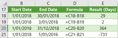
Tip: format the cell to General or Number to see the number of days between two dates.
Note: the ‘result’ is exclusive of the start day i.e. it assumes the start day is at the end of that day.
Adding Times to one another
The time being added is input as a time serial number. Notice there are no negative times in the table below. Remember we can’t display negative times. Instead we need to use the math operator to tell Excel to subtract time. See examples below.
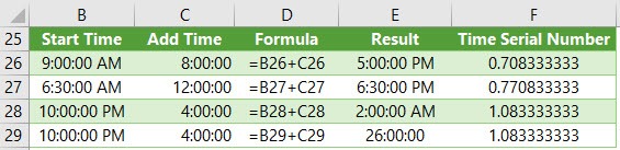
Note: Times that roll over to the next day result in a time-date serial number >= 1. Cell E28 actually contains a time-serial number of 1.08333′, but since the cell is formatted to display time formatted as h:mm:ss, only the time portion is visible.
If you want to show the cumulative time (like cell E29) then you need to surround the ‘h’ part of the time format in square brackets like so: [h]:mm:ss
Subtracting Time from Times
Notice the last result in the table below shows ######, this is because it results in a negative time and Excel can’t display that, but notice it can return a negative time serial number. More on how to solve this later.
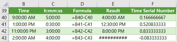
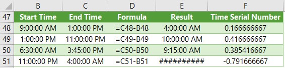
Subtracting Times from one another
Again, here the last result shows ###### because it results in a negative time.
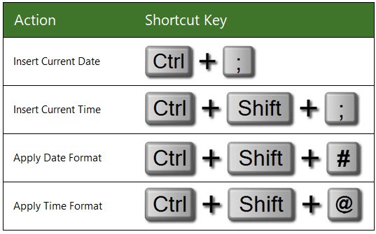
Excel Date and Time Shortcuts
‘Good to Know’ Stuff about Excel Date and Time
— Dates prior to 1st January 1900 are not recognised in Excel.
— A negative date will display in the cell as #######
— Times stored without a date effectively inherit the date 0 Jan 1900 i.e. the month is Jan and the year 1900 and the day is zero. Remember, there are no dates prior to 1/1/1900 from Excel’s perspective. This means that times stored without a date e.g. 0.50 for 12:00 PM is the equivalent of 0 Jan 1900 12:00 PM.
This is important because if you try to take 14 hours from 12 hours (without a date) you’ll get the dreaded ###### display in the cell, because negative dates and times cannot be displayed. We’ll cover workarounds for this later, but for now keep in mind that math on dates and time that result in negative date-time serial numbers cannot be formatted as a date.
Date Modes
— Excel actually has two date modes. The other mode is called 1904 Date System and is used for compatibility with Excel 2008 for Mac and earlier Mac versions. You can change the date system in the Advanced Options.
In the 1904 date system dates are calculated using 1st January 1904 as the starting point. The difference between the two date systems is 1,462 days. This means that the serial number of a date in the 1900 date system is always 1,462 days greater than the serial number of the same date in the 1904 date system. 1,462 days is equal to four years and one day (including one leap day).
Caution; the date setting you choose applies to all dates within the workbook. You can’t mix and match modes and you shouldn’t reference workbooks that use a different date system in formulas.
Bottom line; don’t use the 1904 date system unless absolutely necessary! Click here for more on date systems in Excel.
— Excel applies date number formats based on your system region settings. For example, my system is set to display dates in dd/mm/yyyy format, but if you’re in the U.S. your system is likely to format them as mm/dd/yyyy. Excel will automatically convert the format of date serial numbers to suit your system settings as long as it’s one of the default date formats and not a custom number format.
More Excel Date and Time Tips
This post is just the beginning, the next steps in mastering Excel Date and Time are below:
- Every Excel Date and Time Function explained
- Formatting Date and Time in Excel
- Common Date and Time Calculations
Tip: Avoid waiting, download the workbook and get the above topics now.
Enter your email address below to download the comprehensive Excel workbook and PDF.
By submitting your email address you agree that we can email you our Excel newsletter.
Excel for Microsoft 365 Excel for Microsoft 365 for Mac Excel for the web Excel 2021 Excel 2021 for Mac Excel 2019 Excel 2019 for Mac Excel 2016 Excel 2016 for Mac Excel 2013 Excel 2010 Excel 2007 Excel for Mac 2011 Excel Starter 2010 More…Less
To get detailed information about a function, click its name in the first column.
Note: Version markers indicate the version of Excel a function was introduced. These functions aren’t available in earlier versions. For example, a version marker of 2013 indicates that this function is available in Excel 2013 and all later versions.
|
Function |
Description |
|
DATE function |
Returns the serial number of a particular date |
|
DATEDIF function |
Calculates the number of days, months, or years between two dates. This function is useful in formulas where you need to calculate an age. |
|
DATEVALUE function |
Converts a date in the form of text to a serial number |
|
DAY function |
Converts a serial number to a day of the month |
|
DAYS function |
Returns the number of days between two dates |
|
DAYS360 function |
Calculates the number of days between two dates based on a 360-day year |
|
EDATE function |
Returns the serial number of the date that is the indicated number of months before or after the start date |
|
EOMONTH function |
Returns the serial number of the last day of the month before or after a specified number of months |
|
HOUR function |
Converts a serial number to an hour |
|
ISOWEEKNUM function |
Returns the number of the ISO week number of the year for a given date |
|
MINUTE function |
Converts a serial number to a minute |
|
MONTH function |
Converts a serial number to a month |
|
NETWORKDAYS function |
Returns the number of whole workdays between two dates |
|
NETWORKDAYS.INTL function |
Returns the number of whole workdays between two dates using parameters to indicate which and how many days are weekend days |
|
NOW function |
Returns the serial number of the current date and time |
|
SECOND function |
Converts a serial number to a second |
|
TIME function |
Returns the serial number of a particular time |
|
TIMEVALUE function |
Converts a time in the form of text to a serial number |
|
TODAY function |
Returns the serial number of today’s date |
|
WEEKDAY function |
Converts a serial number to a day of the week |
|
WEEKNUM function |
Converts a serial number to a number representing where the week falls numerically with a year |
|
WORKDAY function |
Returns the serial number of the date before or after a specified number of workdays |
|
WORKDAY.INTL function |
Returns the serial number of the date before or after a specified number of workdays using parameters to indicate which and how many days are weekend days |
|
YEAR function |
Converts a serial number to a year |
|
YEARFRAC function |
Returns the year fraction representing the number of whole days between start_date and end_date |


Important: The calculated results of formulas and some Excel worksheet functions may differ slightly between a Windows PC using x86 or x86-64 architecture and a Windows RT PC using ARM architecture. Learn more about the differences.
Need more help?
 Dates and times are two of the most common data types people work with in Excel, but they are also possibly the most frustrating to work with, especially if you are new to Excel and still learning. This is because Excel uses a serial number to represent the date instead of a proper month, day, or year, nevermind hours, minutes, or seconds. It’s made more complicated by the fact that dates are also days of the week, like Monday or Friday, even though Excel doesn’t explicitly store that information in the cells. Here is the definitive guide to working with dates and times in Excel…
How Excel Stores Dates
The source of most of the confusion around dates and times in Excel comes from the way that the program stores the information. You’d expect it to remember the month, the day, and the year for dates, but that’s not how it works…
Excel stores dates as a serial number that represents the number of days that have taken place since the beginning of the year 1900. This means that January 1, 1900 is really just a 1. January 2, 1900 is 2. By the time we get all the way to the present decade, the numbers have gotten pretty big… September 10, 2013 is stored as 41527.
Importantly, any date before January 1, 1900 is not recognized as a date in Excel. There are no “negative” date serial numbers on the number line.
It seems confusing, but it makes it a lot easier to add, subtract, and count days. A week from September 10, 2013 (September 17, 2013), is just 41527 + 7 days, or 41534.
How Excel Stores Times
Excel stores times using the exact same serial numbering format as with dates. Days start at midnight (12:00am or 0:00 hours). Since each hour is 1/24 of a day, it is represented as that decimal value: 0.041666…
That means that 9:00am (09:00 hours) on September 10, 2013 will be stored as 41527.375.
When a time is specified without a date, Excel stores it as if it occurred on January 0, 1900. In other words, 3:00pm (15:00 hours) is stored as 0.625. This can make doing math for time-only values (that have no date) challenging, since subtracting 6 hours (6:00) from 3:00am (03:00 hours) will become negative and count as an error: 0.125 – 0.25 = -0.125, which is displayed as #########.
Minutes and seconds in Excel work the same way as hours…
A minute is 1/60 of an hour, which is 1/24 of a day, or 1/1440 of a day in total, which calculates to 0.00069444…
A second is 1/60 of an minute, which is 1/60 of an hour, which is 1/24 of a day, or 1/86400 of a day in total, which calculates to 0.00001157407…
Working with Dates and Times
DATE() and TIME()
Serial numbers aren’t all that intuitive to use. Fortunately, Excel has a set of functions to make it easier to find and use dates and times, starting with DATE and TIME. The syntax is as follows:
=DATE(year, month, day)
=TIME(hours, minutes, seconds)
For both functions, specify the year, month, and day, or hours, minutes, and seconds as numbers. For example, September 10, 2013 can be entered as:
=DATE(2013,9,10)
It will be stored as 41527, which means that it is technically storing 12:00am on September 10, 2013.
For times, 6:00pm (18:00 hours) can be entered as:
=TIME(18,0,0)
It will be stored as 0.75, which means that it is technically storing 6:00pm on January 0, 1900.
If we want to represent a specific time and date, we can add the two functions together. For example, 6:00pm (18:00 hours) on September 10, 2013 can be entered as:
=DATE(2013,9,10)+TIME(18,0,0)
It will be calculate as 41527.75, which means Excel is storing exactly the date we want…
Additional Date and Time Setting Functions
Excel has a few additional functions to make declaring dates easier.
TODAY()
The TODAY function always returns the current date’s serial number. The TODAY function is just entered as:
=TODAY()
This article was written at 6:30pm (18:30 hours) on September 24, 2013, and the TODAY function calculated to 41541. That means that it is technically storing 12:00am on September 24, 2013.
NOW()
A similar function called NOW always returns the current date and time’s serial number. The NOW function is just entered as:
=NOW()
Again, at 6:30pm (18:30 hours) on September 24, 2013, the function calculated to 41541.77081333… NOW stores the exact time and date, down to the second.
EDATE() and EOMONTH()
The EDATE function gives the date the specified number of months away from the input date. The EOMONTH function gives the date of the last day of the month. It can do so for the current month or a number of months in the future or the past. The syntax for each is as follows:
=EDATE(start_date, months)
=EOMONTH(start_date, months)
The start_date can be any date-formatted cell reference or date serial number.
The months field can be any number, though only the integer value will be used (e.g. it treats 2.8 as 2).
The EDATE and EOMONTH functions strip the time value from the date. For example, For example, if cell A1 stores September 10, 2013, we can get the value 2 months ahead as follows:
=EDATE(A1,2)
Returns 12:00am (0:00 hours) on November 10, 2013, or 41588. This function works even though the months have different numbers of days (September and November have 30, October has 31).
=EOMONTH(A1,2)
Returns 12:00am (0:00 hours) on November 30, 2013, or 41588. Again, this function works even though the months have different numbers of days.
WORKDAY()
Occasionally, it may be useful to count ahead based on work-days (Monday-Friday) instead of all 7 days of the week… For that, Excel has provided WORKDAY. The syntax for WORKDAY is as follows:
=WORKDAY(start_date, days, [holidays])
The start_date is as above.
The days input is the number of workdays ahead (or behind) of the present day you would like to move.
The [holidays] input is optional, but lets you disqualify specific days (like Thanksgiving or Christmas, for example), which might otherwise fall during the work week. These are date serial numbers provided in an array bounded by brackets: { }. To specify multiple holidays, the dates must be held in cells – it is not possible to put multiple DATE functions in an array.
For example, let’s find the date 6 work days before 6:00pm (18:00 hours) on September 10, 2013 (stored in cell A1). Monday, September 2nd is Labor Day, so let’s include that as a holiday:
=WORKDAY(A1,-6,DATE(2013,9,2))
Returns 12:00am (0:00 hours) on August 30, 2013, or 41516. (Note that the function strips the time portion of the date.)
WORKDAY.INTL() (Excel 2010 and newer)
For newer versions of Excel (2010 and later), there is another version of WORKDAY called WORKDAY.INTL. WORKDAY.INTL works just like WORKDAY, but it adds the ability to customize the definition of the “weekend”. The syntax for WORKDAY.INTL is as follows:
=WORKDAY.INTL(start_date, days, [weekend], [holidays])
The start_date, days, and [holidays] inputs work just like the normal WORKDAY function.
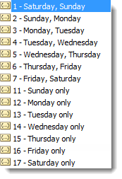
The [weekend] input has the following options:
Retrieving Dates in Excel
DAY(), MONTH(), and YEAR()
Now we know how define dates, but we still need to be able to work with them. Serial numbers don’t make it easy to extract months, years, and days, nevermind hours, minutes, and seconds. That’s why Excel has specific functions for pulling out each of these values. For working with the calendar, there is DAY, MONTH, and YEAR. The syntax is simple:
=DAY(serial_number)
=MONTH(serial_number)
=YEAR(serial_number)
The serial_number in each can be any date-formatted cell reference. For example, if cell A1 stores September 10, 2013, we can use each of the formulas in turn:
=DAY(A1)
Returns 10 as a numeric value.
=MONTH(A1)
Returns 9 as a numeric value.
=YEAR(A1)
Returns 2013 as a numeric value.
We could have also given the direct serial number for September 10, 2013:
=DAY(41527)
Returns 10 as a numeric value.
Retrieving Times in Excel
HOUR(), MINUTE(), and SECOND()
For times, the process is very similar. Excel has function to retrieve the hours, minutes, and seconds from a time stamp, conveniently named HOUR, MINUTE, and SECOND. The syntax is identical:
=HOUR(serial_number)
=MINUTE(serial_number)
=SECOND(serial_number)
The serial_number in each can be any time/date-formatted cell reference. For example, if A1 stores 6:15:30pm (18:15 hours, 30 seconds) on September 10, 2013, we can use each of the formulas in turn:
=HOUR(A1)
Returns 18 as a numeric value.
=MINUTE(A1)
Returns 15 as a numeric value.
=SECOND(A1)
Returns 30 as a numeric value.
We could have also given the direct serial number for 6:15:30pm (18:15 hours, 30 seconds) on September 10, 2013:
=SECOND(41527.7607638889)
Returns 30 as a numeric value.
Additional Date Retrieving Functions
WEEKDAY() and WEEKNUM()
Dates don’t just have month and year information. They also encode indirect information… September 10, 2013 happens to also be a Tuesday. Excel has a few of functions to work with the week aspect of dates: WEEKDAY and WEEKNUM. The syntax is as follows:
=WEEKDAY(serial_number, [return_type])
=WEEKNUM(serial_number, [return_type])
The serial_number in each can be any date-formatted cell reference. Since [return_type] is optional, each function assumes that each week starts on Sunday. If cell A1 stores September 10, 2013 (a Tuesday), we can use each of the formulas in turn:
=WEEKDAY(A1)
Returns 3, since Tuesday is the 3rd day of a week that starts on Sunday.
=WEEKNUM(A1)
Returns 37, since September 10, 2013 is in the 37th week of 2013, when you start counting weeks from Sunday.
The [return_type] allows you to specify a different default week arrangement. You could let the week start on Monday and run until Sunday, or Saturday until Friday, for example. Excel is annoying, however, and makes the entry different for WEEKDAY and WEEKNUM. The full list of options for WEEKDAY is as follows:
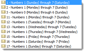
Options 2 and 11 are functionally the same – the first is just there for backwards compatibility with earlier versions of Excel.
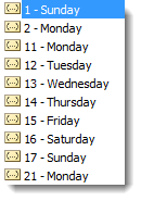
The full list of options for WEEKNUM is as follows:
Counting and Tracking Dates
Dates can be added and subtracted like normal numbers because they’re stored as serial numbers. That lets you count the days between two different dates. Sometimes, though, you need to count by a different metric.
NETWORKDAYS()
Above, we learned about WORKDAY, which lets you move back and forth a set number of workdays, ignoring weekends and holidays. But what if you need to measure the number of workdays between two dates? For that, Excel provides NETWORKDAYS. The formula syntax is as follows:
=NETWORKDAYS(start_date, end_date, [holidays])
The start_date and end_date can be any date-formatted cell reference.
The [holidays] input is optional, but lets you disqualify specific days (like Thanksgiving or Christmas, for example), which might otherwise fall during the work week. These are date serial numbers provided in an array bounded by brackets: { }. To specify multiple holidays, the dates must be held in cells – it is not possible to put multiple DATE functions in an array.
For example, if A1 contains 6:00pm (18:00 hours) on September 10, 2013 and B1 contains 9:00am (9:00 hours) on December 2, 2013, we can use NETWORKDAYS to find the number of workdays between the two dates.
Let’s exclude Columbus Day (October 14, 2013), Veterans Day (November 11, 2013), and Thanksgiving Day (November 28, 2013) as holidays. To do so, we have to store those dates in other cells. Let’s put them in C1, C2, and C3:
=DATE(2013,10,14)
=DATE(2013,11,11)
=DATE(2013,11,28)
Now, we can combine them in the function:
=NETWORKDAYS(A1,B1,C1:C3)
The function returns 57 as a numeric value.
NETWORKDAYS.INTL() (Excel 2010 and newer)
For newer versions of Excel (2010 and later), there is another version of NETWORKDAYS called NETWORKDAYS.INTL. NETWORKDAYS.INTL works just like NETWORKDAYS, but it adds the ability to customize the definition of the “weekend”. The syntax for NETWORKDAYS.INTL is as follows:
=NETWORKDAYS.INTL(start_date, end_date, [weekend], [holidays])
The start_date, end_date, and [holidays] inputs work just like the normal WORKDAY function.
The [weekend] input has the following options:
YEARFRAC()
Sometimes it’s useful to measure how much time has passed in years, but subtracting the YEAR function will only round down to the nearest full year. YEARFRAC takes two dates and provides the portion of the year between them. The syntax is as follows:
=YEARFRAC(start_date, end_date, [basis])
The start_date and end_date can be any date-formatted cell reference.
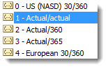
The [basis] input is optional, but lets you specify the “rules” for measuring the difference. Most of the time, you’ll want to use option 1, but here is the full list:
 For example, if A1 contains September 10, 2013 and B1 contains December 2, 2013, we can use YEARFRAC to find the decimal portion of a year between the two dates:
=YEARFRAC(A1,B1,1)
Returns 0.227397260273973.
DATEDIF() (Undocumented Function)
The YEARFRAC function gives you the difference between dates as a fraction of a year, but sometimes you need more control. There is a powerful hidden function in Excel called DATEDIF that can do much more. It can tell you the number of years, months, or days between two dates. It can also track based on only partial inputs, ignoring years or months when calculating days. The syntax for DATEDIF is as follows:
=DATEDIF(start_date, end_date, unit)
The start_date and end_date can be any date-formatted cell reference.
The unit input asks you to specify a string that represents the type of output you want. This is slightly cumbersome, since you must wrap the input in quotes (” “).
For example, if A1 contains September 10, 2012 and B1 contains December 2, 2013, we can use DATEDIF to find the number of full years between the two dates:
=DATEDIF(A1,B1,"Y")
Returns 1 as a numeric value.
Using the same start_date and end_date inputs, here are the output possibilities for DATEDIF using different unit parameters:
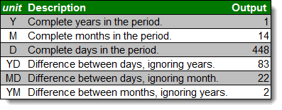
Every time, the unit must be put in quotes (e.g. “Y” or “MD”).
Converting Dates and Times from Text
DATEVALUE() and TIMEVALUE()
All of the above functions work perfectly with date-formatted serial numbers in Excel. Unfortunately, dates and times are often imported into worksheets as text. Most of the assorted functions like MONTH and HOUR are reasonably intelligent about converting on the fly. Occasionally it’s useful to build a date value through concatenation. The two functions Excel provides for this purpose are DATEVALUE and TIMEVALUE. The syntax for each is as follows:
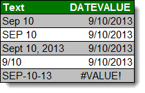
=DATEVALUE(date_text)
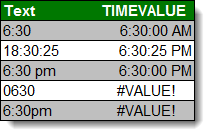
=TIMEVALUE(time_text)
The date_text and time_text accept any text string that looks like a date or time.
This is how DATEVALUE responds to various date_text inputs:
This is how TIMEVALUE responds to various time_text inputs:
Converting Dates and Times to Text
TEXT()
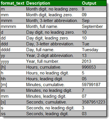
Getting data converted to dates and times is great, but you may also need to get it back out. Sometimes, you need a special format. Other times, you need to look for a date in a text string, and have to match using string tools like FIND and SEARCH. There is one master function for converting dates and times to text strings in Excel, called TEXT. The syntax for TEXT is as follows:
=TEXT(value, format_text)
The value can be any date or time-formatted cell reference.
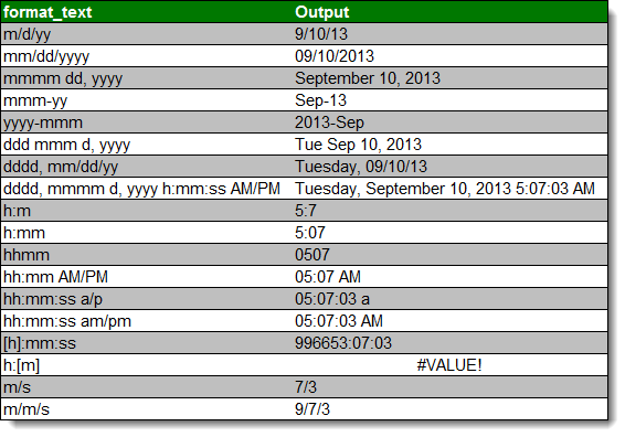
The format_text input has a large number of options, summarized here:
The outputs can be combined with simple formatting characters to produce standard date formats. Using the date 5:07:03am (05:07 hours, 3 seconds) on September 10, 2013, here are examples of possible outputs:
A Common Problem
One issue people frequently run into is that Excel occasionally misinterprets text fields as dates. An example is here:
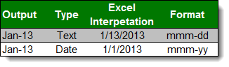
Be careful when entering dates, especially if you are importing from other data sources, to make sure that your “Jan-13” is being stored as January 1, 2013 and not January 13, 2013!
Get the latest Excel tips and tricks by joining the newsletter!
 Andrew Roberts has been solving business problems with Microsoft Excel for over a decade. Excel Tactics is dedicated to helping you master it.
Join the newsletter to stay on top of the latest articles. Sign up and you’ll get a free guide with 10 time-saving keyboard shortcuts!
Other posts in this series…
Содержание
- Работа с функциями даты и времени
- ДАТА
- РАЗНДАТ
- ТДАТА
- СЕГОДНЯ
- ВРЕМЯ
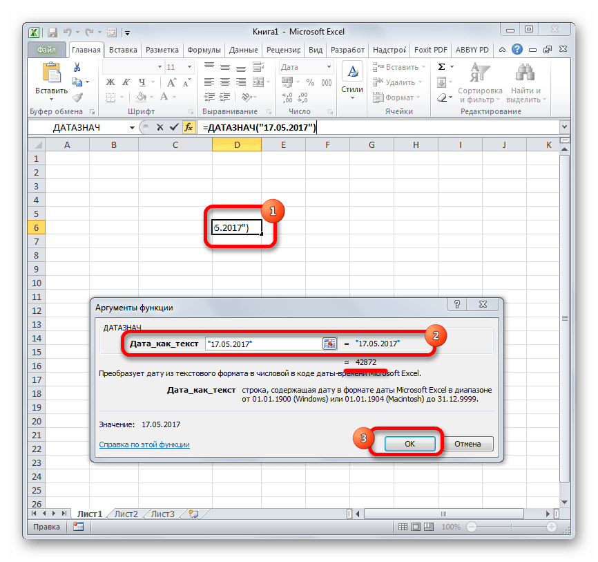
- ДАТАЗНАЧ
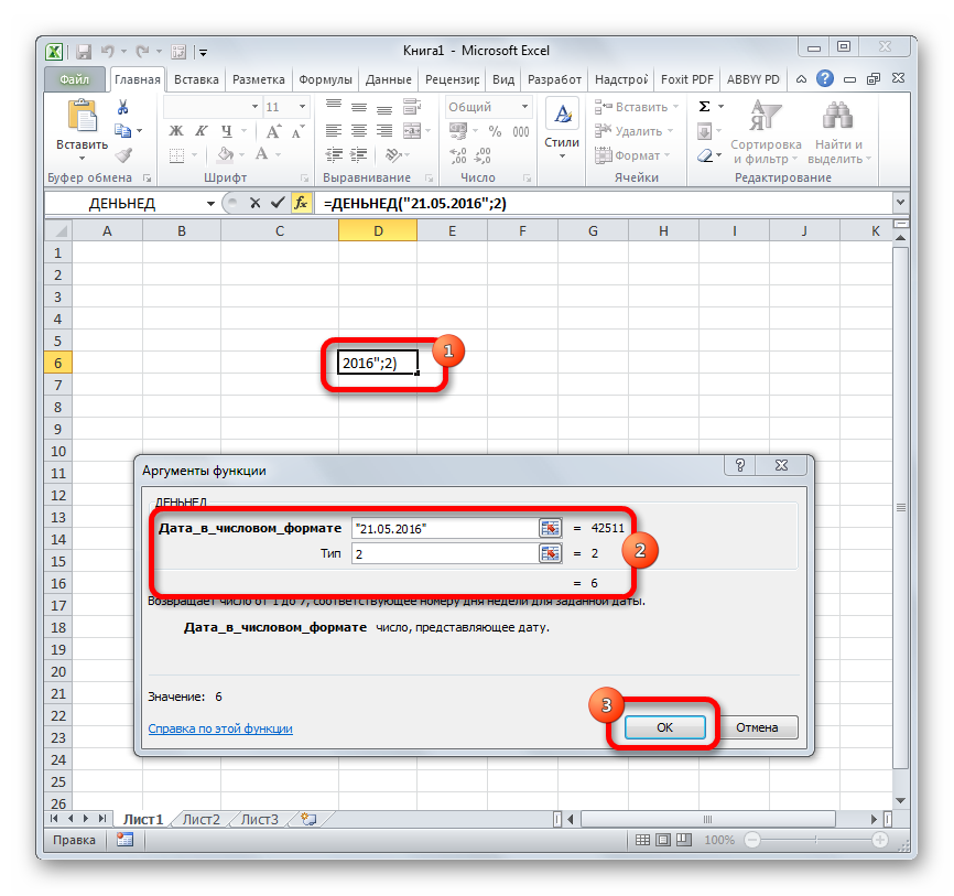
- ДЕНЬНЕД
- НОМНЕДЕЛИ
- ДОЛЯГОДА
- Вопросы и ответы
Одной из самых востребованных групп операторов при работе с таблицами Excel являются функции даты и времени. Именно с их помощью можно проводить различные манипуляции с временными данными. Дата и время зачастую проставляется при оформлении различных журналов событий в Экселе. Проводить обработку таких данных – это главная задача вышеуказанных операторов. Давайте разберемся, где можно найти эту группу функций в интерфейсе программы, и как работать с самыми востребованными формулами данного блока.
Работа с функциями даты и времени
Группа функций даты и времени отвечает за обработку данных, представленных в формате даты или времени. В настоящее время в Excel насчитывается более 20 операторов, которые входят в данный блок формул. С выходом новых версий Excel их численность постоянно увеличивается.
Любую функцию можно ввести вручную, если знать её синтаксис, но для большинства пользователей, особенно неопытных или с уровнем знаний не выше среднего, намного проще вводить команды через графическую оболочку, представленную Мастером функций с последующим перемещением в окно аргументов.
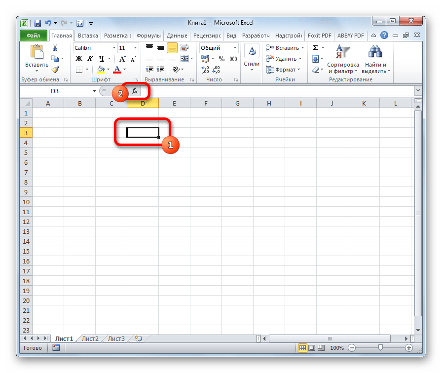
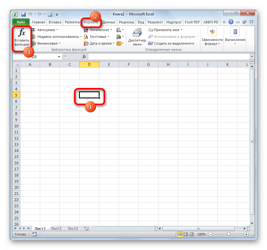
- Для введения формулы через Мастер функций выделите ячейку, где будет выводиться результат, а затем сделайте щелчок по кнопке «Вставить функцию». Расположена она слева от строки формул.
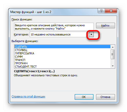
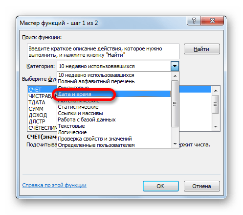
- После этого происходит активация Мастера функций. Делаем клик по полю «Категория».
- Из открывшегося списка выбираем пункт «Дата и время».
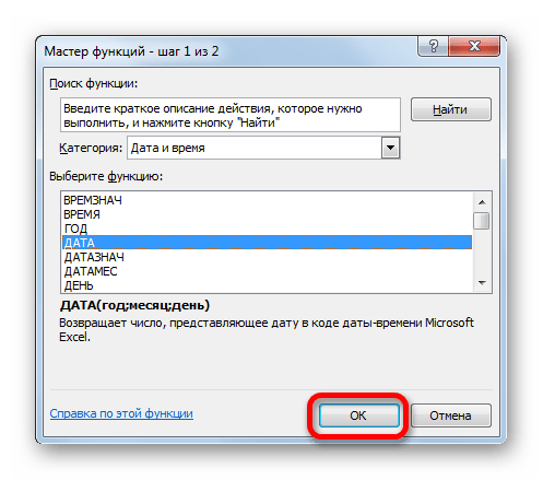
- После этого открывается перечень операторов данной группы. Чтобы перейти к конкретному из них, выделяем нужную функцию в списке и жмем на кнопку «OK». После выполнения перечисленных действий будет запущено окно аргументов.
Кроме того, Мастер функций можно активировать, выделив ячейку на листе и нажав комбинацию клавиш Shift+F3. Существует ещё возможность перехода во вкладку «Формулы», где на ленте в группе настроек инструментов «Библиотека функций» следует щелкнуть по кнопке «Вставить функцию».
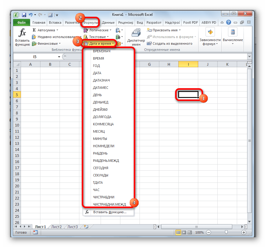
Имеется возможность перемещения к окну аргументов конкретной формулы из группы «Дата и время» без активации главного окна Мастера функций. Для этого выполняем перемещение во вкладку «Формулы». Щёлкаем по кнопке «Дата и время». Она размещена на ленте в группе инструментов «Библиотека функций». Активируется список доступных операторов в данной категории. Выбираем тот, который нужен для выполнения поставленной задачи. После этого происходит перемещение в окно аргументов.
Урок: Мастер функций в Excel
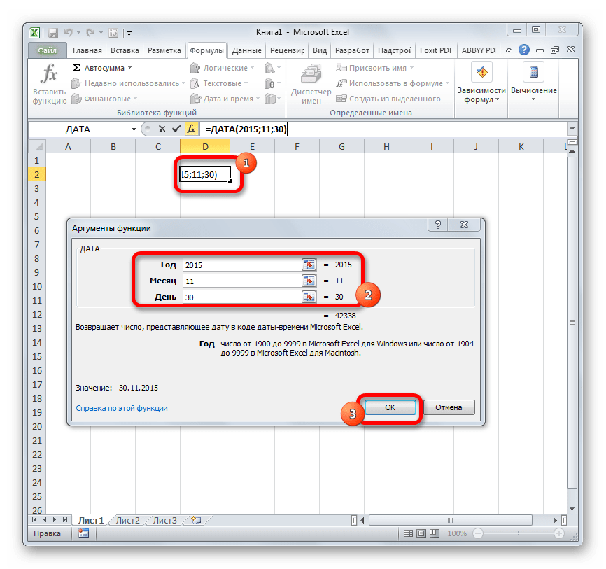
ДАТА
Одной из самых простых, но вместе с тем востребованных функций данной группы является оператор ДАТА. Он выводит заданную дату в числовом виде в ячейку, где размещается сама формула.
Его аргументами являются «Год», «Месяц» и «День». Особенностью обработки данных является то, что функция работает только с временным отрезком не ранее 1900 года. Поэтому, если в качестве аргумента в поле «Год» задать, например, 1898 год, то оператор выведет в ячейку некорректное значение. Естественно, что в качестве аргументов «Месяц» и «День» выступают числа соответственно от 1 до 12 и от 1 до 31. В качестве аргументов могут выступать и ссылки на ячейки, где содержатся соответствующие данные.

Для ручного ввода формулы используется следующий синтаксис:
=ДАТА(Год;Месяц;День)
Близки к этой функции по значению операторы ГОД, МЕСЯЦ и ДЕНЬ. Они выводят в ячейку значение соответствующее своему названию и имеют единственный одноименный аргумент.
РАЗНДАТ
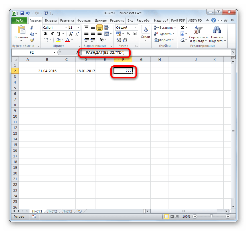
Своего рода уникальной функцией является оператор РАЗНДАТ. Он вычисляет разность между двумя датами. Его особенность состоит в том, что этого оператора нет в перечне формул Мастера функций, а значит, его значения всегда приходится вводить не через графический интерфейс, а вручную, придерживаясь следующего синтаксиса:
=РАЗНДАТ(нач_дата;кон_дата;единица)
Из контекста понятно, что в качестве аргументов «Начальная дата» и «Конечная дата» выступают даты, разницу между которыми нужно вычислить. А вот в качестве аргумента «Единица» выступает конкретная единица измерения этой разности:
- Год (y);
- Месяц (m);
- День (d);
- Разница в месяцах (YM);
- Разница в днях без учета годов (YD);
- Разница в днях без учета месяцев и годов (MD).
Урок: Количество дней между датами в Excel
ЧИСТРАБДНИ
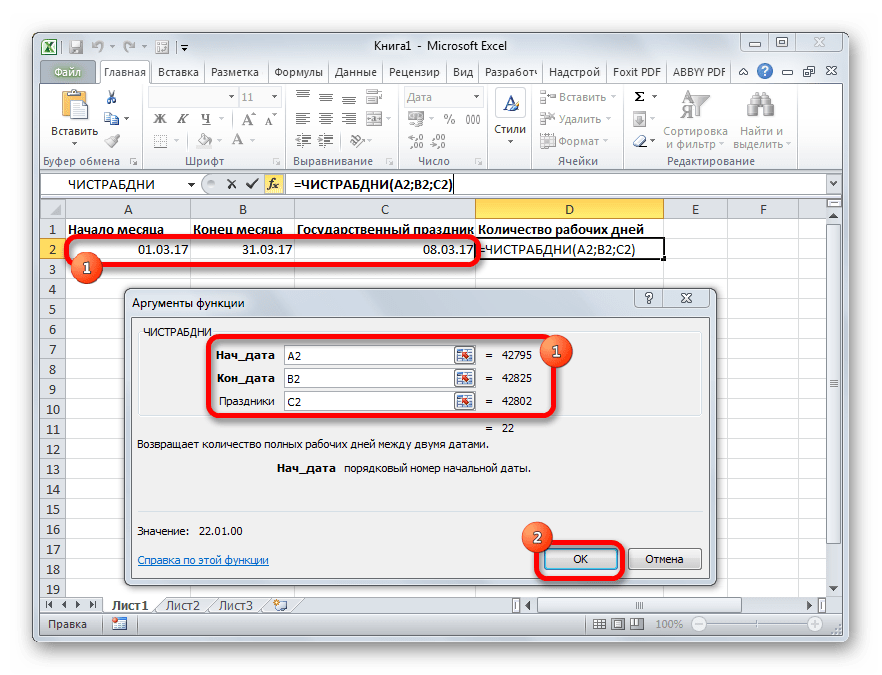
В отличии от предыдущего оператора, формула ЧИСТРАБДНИ представлена в списке Мастера функций. Её задачей является подсчет количества рабочих дней между двумя датами, которые заданы как аргументы. Кроме того, имеется ещё один аргумент – «Праздники». Этот аргумент является необязательным. Он указывает количество праздничных дней за исследуемый период. Эти дни также вычитаются из общего расчета. Формула рассчитывает количество всех дней между двумя датами, кроме субботы, воскресенья и тех дней, которые указаны пользователем как праздничные. В качестве аргументов могут выступать, как непосредственно даты, так и ссылки на ячейки, в которых они содержатся.
Синтаксис выглядит таким образом:
=ЧИСТРАБДНИ(нач_дата;кон_дата;[праздники])
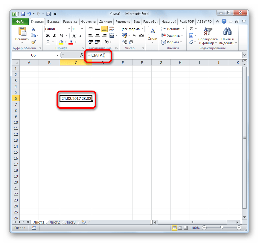
ТДАТА
Оператор ТДАТА интересен тем, что не имеет аргументов. Он в ячейку выводит текущую дату и время, установленные на компьютере. Нужно отметить, что это значение не будет обновляться автоматически. Оно останется фиксированным на момент создания функции до момента её перерасчета. Для перерасчета достаточно выделить ячейку, содержащую функцию, установить курсор в строке формул и кликнуть по кнопке Enter на клавиатуре. Кроме того, периодический пересчет документа можно включить в его настройках. Синтаксис ТДАТА такой:
=ТДАТА()
СЕГОДНЯ
Очень похож на предыдущую функцию по своим возможностям оператор СЕГОДНЯ. Он также не имеет аргументов. Но в ячейку выводит не снимок даты и времени, а только одну текущую дату. Синтаксис тоже очень простой:
=СЕГОДНЯ()
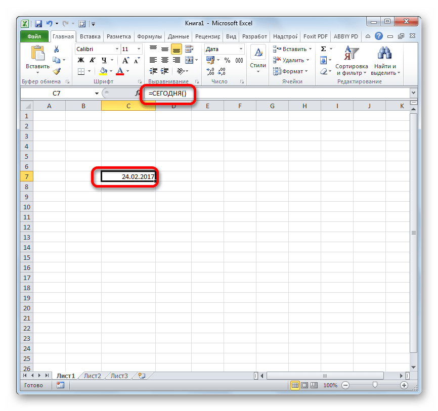
Эта функция, так же, как и предыдущая, для актуализации требует пересчета. Перерасчет выполняется точно таким же образом.
ВРЕМЯ
Основной задачей функции ВРЕМЯ является вывод в заданную ячейку указанного посредством аргументов времени. Аргументами этой функции являются часы, минуты и секунды. Они могут быть заданы, как в виде числовых значений, так и в виде ссылок, указывающих на ячейки, в которых хранятся эти значения. Эта функция очень похожа на оператор ДАТА, только в отличии от него выводит заданные показатели времени. Величина аргумента «Часы» может задаваться в диапазоне от 0 до 23, а аргументов минуты и секунды – от 0 до 59. Синтаксис такой:
=ВРЕМЯ(Часы;Минуты;Секунды)
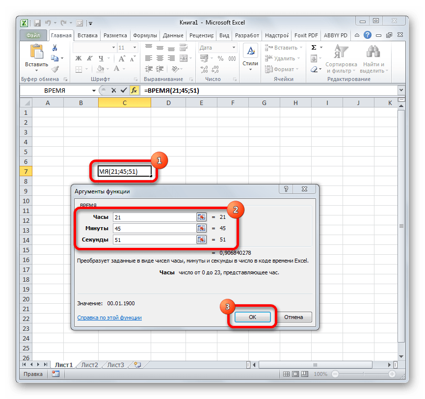
Кроме того, близкими к этому оператору можно назвать отдельные функции ЧАС, МИНУТЫ и СЕКУНДЫ. Они выводят на экран величину соответствующего названию показателя времени, который задается единственным одноименным аргументом.
ДАТАЗНАЧ
Функция ДАТАЗНАЧ очень специфическая. Она предназначена не для людей, а для программы. Её задачей является преобразование записи даты в обычном виде в единое числовое выражение, доступное для вычислений в Excel. Единственным аргументом данной функции выступает дата как текст. Причем, как и в случае с аргументом ДАТА, корректно обрабатываются только значения после 1900 года. Синтаксис имеет такой вид:
=ДАТАЗНАЧ (дата_как_текст)
ДЕНЬНЕД
Задача оператора ДЕНЬНЕД – выводить в указанную ячейку значение дня недели для заданной даты. Но формула выводит не текстовое название дня, а его порядковый номер. Причем точка отсчета первого дня недели задается в поле «Тип». Так, если задать в этом поле значение «1», то первым днем недели будет считаться воскресенье, если «2» — понедельник и т.д. Но это не обязательный аргумент, в случае, если поле не заполнено, то считается, что отсчет идет от воскресенья. Вторым аргументом является собственно дата в числовом формате, порядковый номер дня которой нужно установить. Синтаксис выглядит так:
=ДЕНЬНЕД(Дата_в_числовом_формате;[Тип])
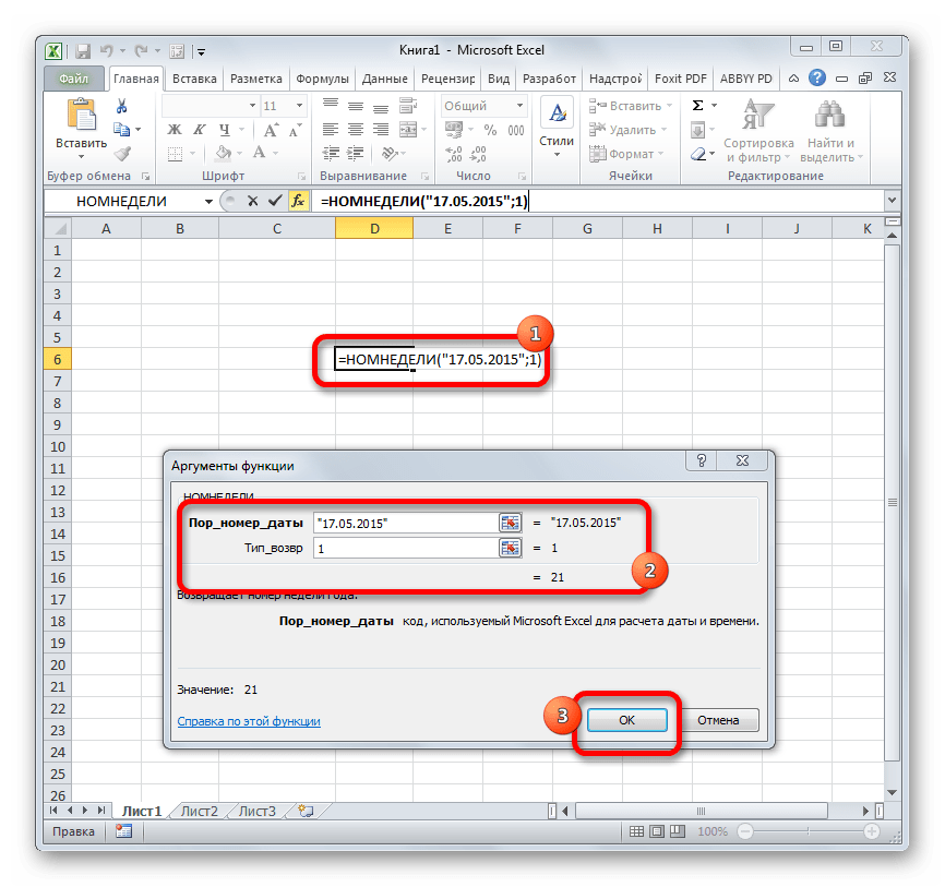
НОМНЕДЕЛИ
Предназначением оператора НОМНЕДЕЛИ является указание в заданной ячейке номера недели по вводной дате. Аргументами является собственно дата и тип возвращаемого значения. Если с первым аргументом все понятно, то второй требует дополнительного пояснения. Дело в том, что во многих странах Европы по стандартам ISO 8601 первой неделей года считается та неделя, на которую приходится первый четверг. Если вы хотите применить данную систему отсчета, то в поле типа нужно поставить цифру «2». Если же вам более по душе привычная система отсчета, где первой неделей года считается та, на которую приходится 1 января, то нужно поставить цифру «1» либо оставить поле незаполненным. Синтаксис у функции такой:
=НОМНЕДЕЛИ(дата;[тип])
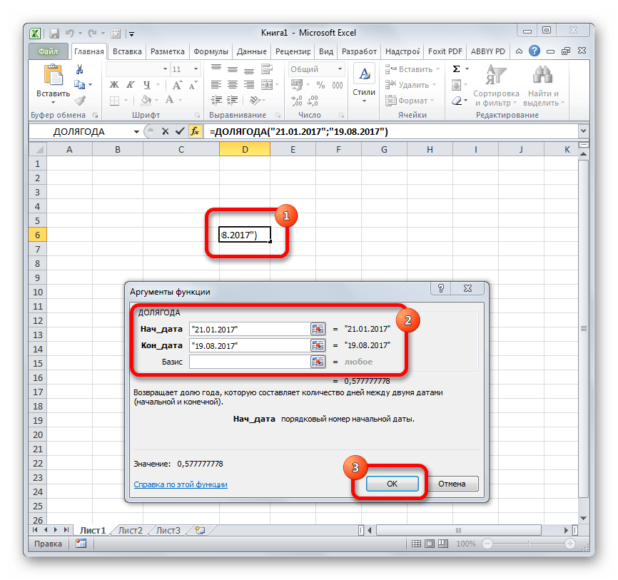
ДОЛЯГОДА
Оператор ДОЛЯГОДА производит долевой расчет отрезка года, заключенного между двумя датами ко всему году. Аргументами данной функции являются эти две даты, являющиеся границами периода. Кроме того, у данной функции имеется необязательный аргумент «Базис». В нем указывается способ вычисления дня. По умолчанию, если никакое значение не задано, берется американский способ расчета. В большинстве случаев он как раз и подходит, так что чаще всего этот аргумент заполнять вообще не нужно. Синтаксис принимает такой вид:
=ДОЛЯГОДА(нач_дата;кон_дата;[базис])
Мы прошлись только по основным операторам, составляющим группу функций «Дата и время» в Экселе. Кроме того, существует ещё более десятка других операторов этой же группы. Как видим, даже описанные нами функции способны в значительной мере облегчить пользователям работу со значениями таких форматов, как дата и время. Данные элементы позволяют автоматизировать некоторые расчеты. Например, по введению текущей даты или времени в указанную ячейку. Без овладения управлением данными функциями нельзя говорить о хорошем знании программы Excel.