What is data validation in excel - Word и Excel - помощь в работе с программами

Use data validation to restrict the type of data or the values that users enter into a cell, like a dropdown list.

Try it!

Select the cell(s) you want to create a rule for.
Select Data >Data Validation.
On the Settings tab, under Allow, select an option:
- Whole Number — to restrict the cell to accept only whole numbers.
- Decimal — to restrict the cell to accept only decimal numbers.
- List — to pick data from the drop-down list.
- Date — to restrict the cell to accept only date.
- Time — to restrict the cell to accept only time.
- Text Length — to restrict the length of the text.
- Custom – for custom formula.
Under Data, select a condition.
Set the other required values based on what you chose for Allow and Data.
Select the Input Message tab and customize a message users will see when entering data.
Select the Show input message when cell is selected checkbox to display the message when the user selects or hovers over the selected cell(s).
Select the Error Alert tab to customize the error message and to choose a Style.
Select OK.

Now, if the user tries to enter a value that is not valid, an Error Alert appears with your customized message.

Download our examples

Download an example workbook with all data validation examples in this article

If you’re creating a sheet that requires users to enter data, you might want to restrict entry to a certain range of dates or numbers, or make sure that only positive whole numbers are entered. Excel can restrict data entry to certain cells by using data validation, prompt users to enter valid data when a cell is selected, and display an error message when a user enters invalid data.

Restrict data entry

Select the cells where you want to restrict data entry.
On the Data tab, click Data Validation > Data Validation.

Note: If the validation command is unavailable, the sheet might be protected or the workbook might be shared. You cannot change data validation settings if your workbook is shared or your sheet is protected. For more information about workbook protection, see Protect a workbook.
In the Allow box, select the type of data you want to allow, and fill in the limiting criteria and values.

Note: The boxes where you enter limiting values will be labeled based on the data and limiting criteria that you have chosen. For example, if you choose Date as your data type, you will be able to enter limiting values in minimum and maximum value boxes labeled Start Date and End Date.

Prompt users for valid entries

When users click in a cell that has data entry requirements, you can display a message that explains what data is valid.

Select the cells where you want to prompt users for valid data entries.
On the Data tab, click Data Validation > Data Validation.

Note: If the validation command is unavailable, the sheet might be protected or the workbook might be shared. You cannot change data validation settings if your workbook is shared or your sheet is protected. For more information about workbook protection, see Protect a workbook.
On the Input Message tab, select the Show input message when cell is selected check box.
In the Title box, type a title for your message.
In the Input message box, type the message that you want to display.

Display an error message when invalid data is entered

If you have data restrictions in place and a user enters invalid data into a cell, you can display a message that explains the error.

Select the cells where you want to display your error message.
On the Data tab, click Data Validation > Data Validation.

Note: If the validation command is unavailable, the sheet might be protected or the workbook might be shared. You cannot change data validation settings if your workbook is shared or your sheet is protected. For more information about workbook protection, see Protect a workbook.
On the Error Alert tab, in the Title box, type a title for your message.
In the Error message box, type the message that you want to display if invalid data is entered.

Do one of the following:

To	On the Style pop-up menu, select
Require users to fix the error before proceeding	Stop
Warn users that data is invalid, and require them to select Yes or No to indicate if they want to continue	Warning
Warn users that data is invalid, but allow them to proceed after dismissing the warning message	Important

Add data validation to a cell or a range

Note: The first two steps in this section are for adding any type of data validation. Steps 3-7 are specifically for creating a drop-down list.

Select one or more cells to validate.
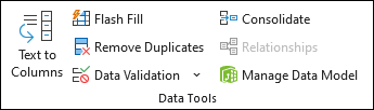
On the Data tab, in the Data Tools group, click Data Validation.
On the Settings tab, in the Allow box, select List.
In the Source box, type your list values, separated by commas. For example, type Low,Average,High.
Make sure that the In-cell dropdown check box is selected. Otherwise, you won’t be able to see the drop-down arrow next to the cell.
To specify how you want to handle blank (null) values, select or clear the Ignore blank check box.
Test the data validation to make sure that it is working correctly. Try entering both valid and invalid data in the cells to make sure that your settings are working as you intended and your messages are appearing when you expect.

Notes:

After you create your drop-down list, make sure it works the way you want. For example, you might want to check to see if the cell is wide enough to show all your entries.
Remove data validation — Select the cell or cells that contain the validation you want to delete, then go to Data > Data Validation and in the data validation dialog press the Clear All button, then click OK.

The following table lists other types of data validation and shows you ways to add it to your worksheets.

To do this:	Follow these steps:
Restrict data entry to whole numbers within limits.	Follow steps 1-2 above. From the Allow list, select Whole number. In the Data box, select the type of restriction that you want. For example, to set upper and lower limits, select between. Enter the minimum, maximum, or specific value to allow. You can also enter a formula that returns a number value. For example, say you’re validating data in cell F1. To set a minimum limit of deductions to two times the number of children in that cell, select greater than or equal to in the Data box and enter the formula, *=2F1, in the Minimum** box.
Restrict data entry to a decimal number within limits.	Follow steps 1-2 above. In the Allow box, select Decimal. In the Data box, select the type of restriction that you want. For example, to set upper and lower limits, select between. Enter the minimum, maximum, or specific value to allow. You can also enter a formula that returns a number value. For example, to set a maximum limit for commissions and bonuses of 6% of a salesperson’s salary in cell E1, select less than or equal to in the Data box and enter the formula, *=E16%, in the Maximum box. Note: To let a user enter percentages, for example 20%, select Decimal in the Allow box, select the type of restriction that you want in the Data box, enter the minimum, maximum, or specific value as a decimal, for example .2, and then display the data validation cell as a percentage by selecting the cell and clicking Percent Style in the Number group on the Home** tab.
Restrict data entry to a date within range of dates.	Follow steps 1-2 above. In the Allow box, select Date. In the Data box, select the type of restriction that you want. For example, to allow dates after a certain day, select greater than. Enter the start, end, or specific date to allow. You can also enter a formula that returns a date. For example, to set a time frame between today’s date and 3 days from today’s date, select between in the Data box, enter =TODAY() in the Start date box, and enter =TODAY()+3 in the End date box.
Restrict data entry to a time within a time frame.	Follow steps 1-2 above. In the Allow box, select Time. In the Data box, select the type of restriction that you want. For example, to allow times before a certain time of day, select less than. Enter the start, end, or specific time to allow. If you want to enter specific times, use the hh:mm time format. For example, say you have cell E2 set up with a start time (8:00 AM), and cell F2 with an end time (5:00 PM), and you want to limit meeting times between those times then select between in the Data box, enter =E2 in the Start time box, and then enter =F2 in the End time box.
Restrict data entry to text of a specified length.	Follow steps 1-2 above. In the Allow box, select Text Length. In the Data box, select the type of restriction that you want. For example, to allow up to a certain number of characters, select less than or equal to. In this case we want to limit entry to 25 characters, so select less than or equal to in the Data box and enter 25 in the Maximum box.
Calculate what is allowed based on the content of another cell.	Follow steps 1-2 above. In the Allow box, select the type of data that you want. In the Data box, select the type of restriction that you want. In the box or boxes below the Data box, click the cell that you want to use to specify what is allowed. For example, to allow entries for an account only if the result won’t go over the budget in cell E1, select Allow >Whole number, Data, less than or equal to, and Maximum >= =E1.

Notes:

The following examples use the Custom option where you write formulas to set your conditions. You don’t need to worry about whatever the Data box shows, as that’s disabled with the Custom option.
The screen shots in this article were taken in Excel 2016; but the functionality is the same in Excel for the web.

To make sure that	Enter this formula
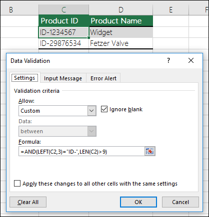
The cell that contains a product ID (C2) always begins with the standard prefix of «ID-» and is at least 10 (greater than 9) characters long.	=AND(LEFT(C2,3)=»ID-«,LEN(C2)>9)
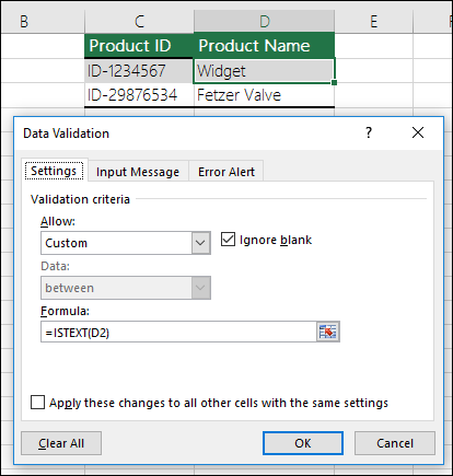
The cell that contains a product name (D2) only contains text.	=ISTEXT(D2)
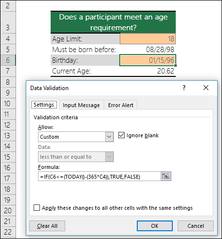
The cell that contains someone’s birthday (B6) has to be greater than the number of years set in cell B4.	*=IF(B6<=(TODAY()-(365B4)),TRUE,FALSE)**
All the data in the cell range A2:A10 contains unique values.	=COUNTIF($A$2:$A$10,A2)=1 Note: You must enter the data validation formula for cell A2 first, then copy A2 to A3:A10 so that the second argument to the COUNTIF will match the current cell. That is the A2)=1 portion will change to A3)=1, A4)=1 and so on. For more information
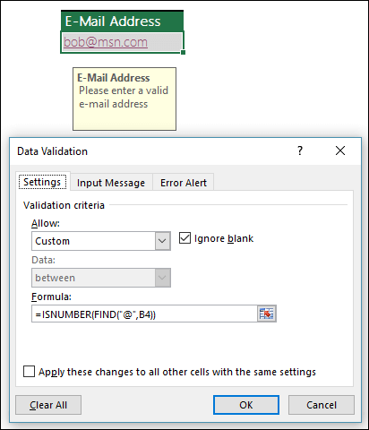
Ensure that an e-mail address entry in cell B4 contains the @ symbol.	=ISNUMBER(FIND(«@»,B4))

Tip: If you’re a small business owner looking for more information on how to get Microsoft 365 set up, visit Small business help & learning.

Want more?

Create a drop-down list

Add or remove items from a drop-down list

Introduction

Data validation is a feature in Excel used to control what a user can enter into a cell. For example, you could use data validation to make sure a value is a number between 1 and 6, make sure a date occurs in the next 30 days, or make sure a text entry is less than 25 characters.

Data validation can simply display a message to a user telling them what is allowed as shown below:

Data validation can also stop invalid user input. For example, if a product code fails validation, you can display a message like this:

In addition, data validation can be used to present the user with a predefined choice in a dropdown menu:

This can be a convenient way to give a user exactly the values that meet requirements.

Data validation controls

Data validation is implemented via rules defined in Excel’s user interface on the Data tab of the ribbon.

Important limitation

It is important to understand that data validation can be easily defeated. If a user copies data from a cell without validation to a cell with data validation, the validation is destroyed (or replaced). Data validation is a good way to let users know what is allowed or expected, but it is not a foolproof way to guarantee input.

Defining data validation rules

Data validation is defined in a window with 3 tabs: Settings, Input Message, and Error Alert:

The settings tab is where you enter validation criteria. There are a number of built-in validation rules with various options, or you can select Custom, and use your own formula to validate input as seen below:

The Input Message tab defines a message to display when a cell with validation rules is selected. This Input Message is completely optional. If no input message is set, no message appears when a user selects a cell with data validation applied. The input message has no effect on what the user can enter — it simply displays a message to let the user know what is allowed or expected.

The Error Alert Tab controls how validation is enforced. For example, when style is set to «Stop», invalid data triggers a window with a message, and the input is not allowed.

The user sees a message like this:

When style is set to Information or Warning, a different icon is displayed with a custom message, but the user can ignore the message and enter values that don’t pass validation. The table below summarizes behavior for each error alert option.

Alert Style	Behavior
Stop	Stops users from entering invalid data in a cell. Users can retry, but must enter a value that passes data validation. The Stop alert window has two options: Retry and Cancel.
Warning	Warns users that data is invalid. The warning does nothing to stop invalid data. The Warning alert window has three options: Yes (to accept invalid data), No (to edit invalid data) and Cancel (to remove the invalid data).
Information	Informs users that data is invalid. This message does nothing to stop invalid data. The Information alert window has 2 options: OK to accept invalid data, and Cancel to remove it.

Data validation options

When a data validation rule is created, there are eight options available to validate user input:

Any Value — no validation is performed. Note: if data validation was previously applied with a set Input Message, the message will still display when the cell is selected, even when Any Value is selected.

Whole Number — only whole numbers are allowed. Once the whole number option is selected, other options become available to further limit input. For example, you can require a whole number between 1 and 10.

Decimal — works like the whole number option, but allows decimal values. For example, with the Decimal option configured to allow values between 0 and 3, values like .5, 2.5, and 3.1 are all allowed.

List — only values from a predefined list are allowed. The values are presented to the user as a dropdown menu control. Allowed values can be hardcoded directly into the Settings tab, or specified as a range on the worksheet.

Date — only dates are allowed. For example, you can require a date between January 1, 2018 and December 31 2021, or a date after June 1, 2018.

Time — only times are allowed. For example, you can require a time between 9:00 AM and 5:00 PM, or only allow times after 12:00 PM.

Text length — validates input based on number of characters or digits. For example, you could require code that contains 5 digits.

Custom — validates user input using a custom formula. In other words, you can write your own formula to validate input. Custom formulas greatly extend the options for data validation. For example, you could use a formula to ensure a value is uppercase, a value contains «xyz», or a date is a weekday in the next 45 days.

The settings tab also includes two checkboxes:

Ignore blank — tells Excel to not validate cells that contain no value. In practice, this setting seems to affect only the command «circle invalid data». When enabled, blank cells are not circled even if they fail validation.

Apply these changes to other cells with the same settings — this setting will update validation applied to other cells when it matches the (original) validation of the cell(s) being edited.

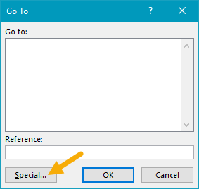
Note: You can also manually select all cells with data validation applied using Go To + Special, as explained below.

Simple drop down menu

You can provide a dropdown menu of options by hardcoding values into the settings box, or selecting a range on the worksheet. For example, to restrict entries to the actions «BUY», «HOLD», or «SELL» you can enter these values separated with commas as seen below:

When applied to a cell in the worksheet, the dropdown menu works like this:

Another way to supply values to a dropdown menu is to use a worksheet reference. For example, with sizes (i.e. small, medium, etc.) in the range F3:F6, you can supply this range directly inside the data validation settings window:

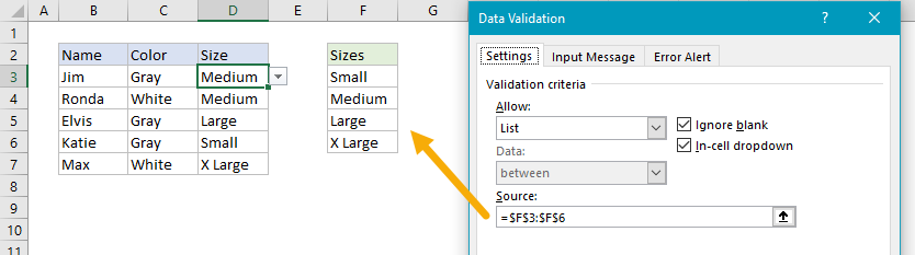
Note the range is entered as an absolute address to prevent it from changing as the data validation is applied to other cells.

Tip: Click the small arrow icon at the far right of the source field to make a selection directly on the worksheet so you don’t have to enter the range manually.

You can also use named ranges to specify values. For example, with the named range called «sizes» for F3:F7, you can enter the name directly in the window, starting with an equal sign:

Named ranges are automatically absolute, so they won’t change as the data validation is applied to different cells. If named ranges are new to you, this page has a good overview and a number of related tips.

Tip — if you use an Excel Table for dropdown values, Excel will expand or contract the table automatically when dropdown values are added or removed. In other words, Excel will automatically keep the dropdown in sync with values in the table as values are changed, added, or removed. If you’re new to Excel Tables, you can see a demo in this video on Table shortcuts.

Data validation with a custom formula

Data validation formulas must be logical formulas that return TRUE when input is valid and FALSE when input is invalid. For example, to allow any number as input in cell A1, you could use the ISNUMBER function in a formula like this:

=ISNUMBER(A1)

If a user enters a value like 10 in A1, ISNUMBER returns TRUE and data validation succeeds. If they enter a value like «apple» in A1, ISNUMBER returns FALSE and data validation fails.

To enable data validation with a formula, selected «Custom» in the settings tab, then enter a formula in the formula bar beginning with an equal sign (=) as usual.

Troubleshooting formulas

Excel ignores data validation formulas that return errors. If a formula isn’t working, and you can’t figure out why, set up dummy formulas to make sure the formula is performing as you expect. Dummy formulas are simply data validation formulas entered directly on the worksheet so that you can see what they return easily. The screen below shows an example:

Once you get the dummy formula working like you want, simply copy and paste it into the data validation formula area.

If this dummy formula idea is confusing to you, watch this video, which shows how to use dummy formulas to perfect conditional formatting formulas. The concept is exactly the same.

Data validation formula examples

The possibilities for data validation custom formulas are virtually unlimited. Here are a few examples to give you some inspiration:

To allow only 5 character values that begin with «z» you could use:

=AND(LEFT(A1)="z",LEN(A1)=5)

This formula returns TRUE only when a code is 5 digits long and starts with «z». The two circled values return FALSE with this formula.

To allow only a date within 30 days of today:

=AND(A1>TODAY(),A1<=(TODAY()+30))

To allow only unique values:

=COUNTIF(range,A1)<2

To allow only an email address

=ISNUMBER(FIND("@",A1)

Data validation to circle invalid entries

Once data validation is applied, you can ask Excel to circle previously entered invalid values. On the Data tab of the ribbon, click Data Validation and select «Circle Invalid Data»:

For example, the screen below shows values circled that fail validation with this custom formula:

=AND(LEFT(A1)="z",LEN(A1)=5)

Find cells with data validation

To find cells with data validation applied, you can use the Go To > Special dialog. Type the keyboard shortcut Control + G, then click the Special button. When the Dialog appears, select «Data Validation»:

Copy data validation from one cell to another

To copy validation from one cell to other cells. Copy the cell(s) normally that contain the data validation you want, then use Paste Special + Validation. Once the dialog appears, type «n» to select validation, or click validation with the mouse.

Note: you can use the keyboard shortcut Control + Alt + V to invoke Paste Special without the mouse.

Clear all data validation

To clear all data validation from a range of cells, make the selection, then click the Data Validation button on the Data tab of the ribbon. Then click the «Clear All» button:

To clear all data validation from a worksheet, select the entire worksheet, then, follow the same steps above.

Источник

Excel data validation is a feature that allows you to control the type of data entered into your worksheet. For example, Excel data validation allows you to limit data entries to a selection from a dropdown list and to restrict certain data entries, such as dates or numbers outside of a predetermined range.

Contents

1 What is data validation in Excel with example?
2 How do you use data validation in Excel?
3 What is data validation used for?
4 What are the 3 types of data validation?
5 What is an example of validation?
6 What is Vlookup in Excel?
7 Why is data validation in Excel important?
8 What is data validation testing?
9 What are the different types of validation?
10 What is data validation process?
11 What is validation method?
12 What are the 8 types of data validation rules?
13 What are validation rules?
14 What is the difference between data verification and data validation?
15 What is data validation in data analysis?
16 How do you validate survey data?
17 What is macro in Excel?
18 What is concatenate in Excel?
19 What is meant by pivot table?
20 What is Freeze Excel?

What is data validation in Excel with example?

Data validation is a feature in Excel used to control what a user can enter into a cell. For example, you could use data validation to make sure a value is a number between 1 and 6, make sure a date occurs in the next 30 days, or make sure a text entry is less than 25 characters.

How do you use data validation in Excel?

How to do data validation in Excel

Open the Data Validation dialog box. Select one or more cells to validate, go to the Data tab > Data Tools group, and click the Data Validation button.
Create an Excel validation rule.
Add an input message (optional)
Display an error alert (optional)

What is data validation used for?

Often, data validation is used as a part of processes such as ETL (Extract, Transform, and Load) where you move data from a source database to a target data warehouse so that you can join it with other data for analysis. Data validation helps ensure that when you perform analysis, your results are accurate.

What are the 3 types of data validation?

Types of validation

Validation type	How it works
Length check	Checks the data isn’t too short or too long
Lookup table	Looks up acceptable values in a table
Presence check	Checks that data has been entered into a field
Range check	Checks that a value falls within the specified range

What is an example of validation?

To validate is to confirm, legalize, or prove the accuracy of something. Research showing that smoking is dangerous is an example of something that validates claims that smoking is dangerous. To establish the soundness, accuracy, or legitimacy of.

What is Vlookup in Excel?

VLOOKUP stands for ‘Vertical Lookup’. It is a function that makes Excel search for a certain value in a column (the so called ‘table array’), in order to return a value from a different column in the same row.

Why is data validation in Excel important?

Excel data validation is a feature that allows you to control the type of data entered into your worksheet.As a result, Excel data validation helps reduce the amount of unstandardized data, errors, or irrelevant information in your worksheet.

Data Validation testing is a process that allows the user to check that the provided data, they deal with, is valid or complete.In simple words, data validation is a part of Database testing, in which individual checks that the entered data valid or not according to the provided business conditions.

What are the different types of validation?

There are 4 main types of validation:

Prospective Validation.
Concurrent Validation.
Retrospective Validation.
Revalidation (Periodic and After Change)

What is data validation process?

Data validation refers to the process of ensuring the accuracy and quality of data. It is implemented by building several checks into a system or report to ensure the logical consistency of input and stored data.

What is validation method?

Method validation is the process used to confirm that the analytical procedure employed for a specific test is suitable for its intended use. Results from method validation can be used to judge the quality, reliability and consistency of analytical results; it is an integral part of any good analytical practice.

What are the 8 types of data validation rules?

Data Validation Rules

dataLength.
dateRange.
matchFromFile.
patternMatch.
range.
reject.
return.
validateDBField.

What are validation rules?

Validation rules verify that the data a user enters in a record meets the standards you specify before the user can save the record. A validation rule can contain a formula or expression that evaluates the data in one or more fields and returns a value of “True” or “False”.

What is the difference between data verification and data validation?

Data verification: to make sure that the data is accurate. Data validation: to make sure that the data is correct.

What is data validation in data analysis?

Data validation means checking the accuracy and quality of source data before using, importing or otherwise processing data. Different types of validation can be performed depending on destination constraints or objectives. Data validation is a form of data cleansing.

How do you validate survey data?

Questionnaire Validation in a Nutshell

Generally speaking the first step in validating a survey is to establish face validity.
The second step is to pilot test the survey on a subset of your intended population.
After collecting pilot data, enter the responses into a spreadsheet and clean the data.

What is macro in Excel?

An Excel macro is an action or a set of actions that you can record, give a name, save and run as many times as you want and whenever you want. Macros help you to save time on repetitive tasks involved in data manipulation and data reports that are required to be done frequently.

What is concatenate in Excel?

The word concatenate is just another way of saying “to combine” or “to join together”. The CONCATENATE function allows you to combine text from different cells into one cell. In our example, we can use it to combine the text in column A and column B to create a combined name in a new column.

What is meant by pivot table?

A pivot table is a powerful data summarization tool that can automatically sort, count, and sum up data stored in tables and display the summarized data.Typically, with a pivot table the user sets up and changes the data summary’s structure by dragging and dropping fields graphically.

What is Freeze Excel?

The Excel Freeze Panes tool allows you to lock your column and/or row headings so that, when you scroll down or over to view the rest of your sheet, the first column and/or top row remain on the screen.

Источник

Microsoft Excel is a powerful tool and is widely useful too. It has various features to ease our work. One such feature is Data Validation. Now suppose you want the user to enter some specific values into the cells and for that, you need to set some pre-defined rules so that the user wouldn’t be able to enter other values and that’s where Data Validation steps in.

Data Validation gives you the control to receive particular inputs from users. We all have encountered using this feature in our day-to-day lives, one such example is while filling out forms in which the age cell will accept numbers similarly name column accepts text with limited characters, and data of birth will have years pre-defined to rule out the ineligible candidates.

Data Validation:

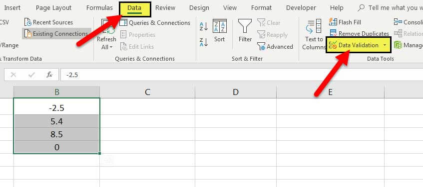
The data validation function can be found in the DATA tab from the excel ribbon(as seen in the picture below).

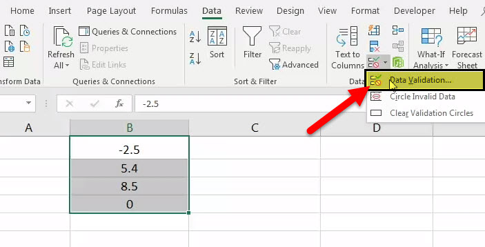
After clicking on the Data Validation, a menu appears.

Select Data Validation and a dialogue box appear.

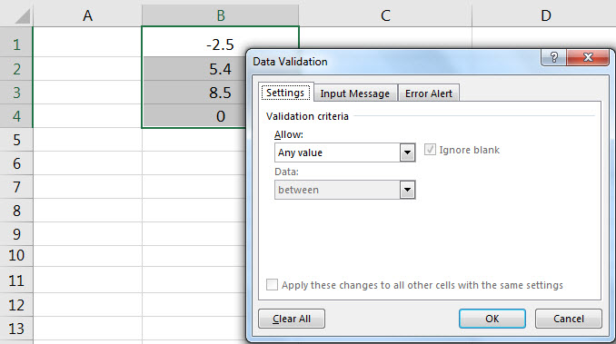
There are 3 tabs in the dialogue box.

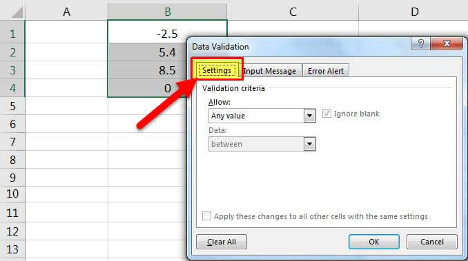
Settings: This will help you to select the data type and the type of data that you want to be filled in the desired row or column.
Input Message: This tab will help to let the user know about the constraints you’ve decided for the row/column. It will alert the user to input the right set of values.
Error Alert: The error alert tab will help the user to know that they had entered invalid data.

Note: The data validation feature is not 100 percent reliable. If you will try to copy the data from cells which has no defined validation rules and then try to paste those cells to cells having data validation then all the validation part get vanished. Basically, validation rules get changed from the corresponding cell based on the copied cell content.

Example of Data Validation

Let’s take the example of filling a form. The form requires your name which has a limitation of 3-7 characters, it requires your date of birth and has a list of cities for the exam centre. Not considering all the other requirements as of now.

The form looks like this.

To apply data validation with a word limit of 3-7 characters for the Name cell.

Step 1: Select the empty cell in front of the Name.

Step 2: From the DATA tab in the ribbon, select Data Validation.

Step 3: A Dialogue box will appear.

Step 4: In the dialogue box from the setting tab, in the dropdown, select Text Length (as shown in the image below).

Step 5: We want our user to enter the name between 3-7 characters, So in the Minimum column we’ll write 3 and in the Maximum column we’ll write 7 and then click OK.

The Name row will now accept only text between 3-7 characters.

To use data validation as Date of Birth:

Step 6: Select the cell in front of Data of Birth in excel.

Step 7: Repeat steps 2 and 3.

Step 8: In this step, instead of selecting text length, you need to select Date (as shown in the image below).

If you want the user must be born between 1st January 2000 to 1st January 2021. Enter the Start date as 1st January 2000 and End date as 1st January 2021.

Step 9: Click OK.

Now, the Date of the Birth row will accept dates between 1st January 2000 to 1st January 2021.

To use data validation as a List:

Step 10: Select the empty cell in front of Exam Centre..

Step 11: Repeat steps 2 and 3.

Step 12: Select List (as shown in the image below).

You want to add “Kanpur”,”Agra”,”Aligarh”,”Lucknow”,”Varanasi” to the list.

Step 13: Add the names in the source column separated by a comma(,).

Step 14: Click OK.

The Exam centre cell will look like this.

You’ve successfully created a form with 3 requirements using Data Validation.

Источник

The data validation in excel helps control the kind of input entered by a user in the worksheet. In other words, the input typed in a specific cell must comply with the criteria set for that cell. Data validation also allows providing instructions to the user about the input to be typed. The cell to which the data validation rule is applied is called a validated cell.

For example, the following data validation rules can be created in certain cells of Excel:

A whole number between 1 (minimum) and 20 (maximum) is allowed.
A date is allowed to be entered which is greater than September 15, 2000 (start date) or lesser than September 15, 2020 (end date).
A text entry is allowed which matches any of the values (“yes,” “no,” and “cannot say”) of a drop-down list.

The pointers “a,” “b,” and “c” are the validating criteria defined for certain cells. If the input in these cells does not correspond to the respective pointer (a, b, or c), an error alert message is displayed by Excel.

Apart from setting the criteria, data validation in excel also allows to create a pre-defined range of inputs (drop-down list). In such cases, the user is asked to select the appropriate option (input) from this range. This ensures that all the data entries follow the same format.

Since the entries of all users are standardized, data validation brings about consistency and reduces errors. The “data validation” option is available in the “data tools” group of the Data tab of Excel.

What is Data Validation in Excel?
- How to Use Data Validation in Excel?
  - Example #1–“Data Validation” Window Explained
  - Example #2–Decimal Number Validation
- Data Formats in Data validation
- The Different Validation Criteria
- The Different Error Alert Styles
- Purpose of Data Validation in Excel
- The Limitations of Data Validation in Excel
- Frequently Asked Questions
- Recommended Articles

How to Use Data Validation in Excel?

Let us consider some examples to understand the working of the data validation feature of Excel.

You can download this Data Validation Excel Template here – Data Validation Excel Template

Example #1–“Data Validation” Window Explained

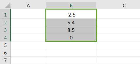
The following image shows a list of numbers in column B. We want to perform the following tasks:

Show how to create a data validation rule on the range B1:B4.
Explain the tabs of the “data validation” window.

The steps explaining the creation of a data validation rule in Excel are listed as follows:

Select the cells on which the data validation rule has to be created. So, select the range B1:B4.
Click the data validation drop-down (in the “data tools” group) from the Data tab of Excel. The same is shown in the following image.
Select “data validation” from the drop-down list.
The “data validation” window appears, as shown in the following image.
The first tab is “settings,” which contains the validation criteria. The same is shown in the succeeding image.
From the drop-down list under “allow,” one can select the data format allowed to the users. The drop-down list under “data” is used for defining the criteria.

For instance, if the input should be entered as a whole number, select the same from the drop-down list under “allow.” Once “whole number” is selected, one can choose the minimum and the maximum range between which this number is allowed to be entered.

Likewise, the desired validation criteria can be defined for the user.

Note: Refer to the topics “The Different Data Formats” and “The Different Validation Criteria” of this article for more information on adding validation criteria.
The checkbox “ignore blank” is selected by default. This selection tells Excel to ignore the blank values.
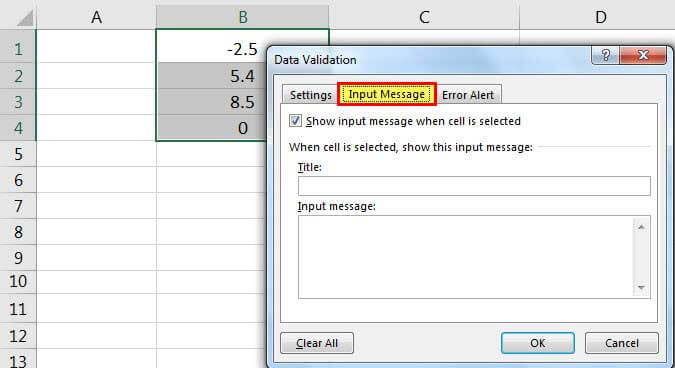
The second tab is “input message,” as shown in the succeeding image. One can enter the “title” and the “input message,” which are displayed when a validated cell is selected.
Note: An “input message” tells the user about the kind of input allowed in a validated cell. However, it is optional to add an input message. But, if one does add an input message, ensure that the checkbox of “show input message when cell is selected” is checked.
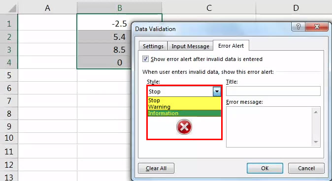
The third tab is “error alert.” In this tab, one can enter the “title” and the “error message” that are displayed on typing invalid data in the validated cell.
From the “style” drop-down, one can select any of the three options, “stop,” “warning” or “information.” These are shown in the succeeding image.

Note 1: An “error message” is a customized message which tells the user that he/she has made an error while typing data in the validated cell. However, it is optional to add an error message. If an error message is added, ensure that the checkbox of “show error alert after invalid data is entered” is checked.

Note 2: In case an error message is not added, Excel displays the default error message, which states that restrictions have been defined for the validated cell.

Note 3: For more information on the error alert styles, refer to the topic “The Different Error Alert Styles” of this article.
Once the entries in the three tabs, “settings,” “input message,” and “error alert” have been defined, click “Ok” in the “data validation” window.
The data validation excel rule is applied to the selected range B1:B4. Likewise, one can create a data validation rule by selecting either a single cell or a range of cells in Excel.

Note: For creating a data validation rule, it is mandatory to enter the validation criteria in the “settings” tab (step 5). However, it is optional to define the tabs “input message” (step 7) and “error alert” (step 8).

Example #2–Decimal Number Validation

Working on the data of example #1, we want to perform the following tasks:

Create a data validation excel rule on cell B1. In this cell, a decimal number greater than or equal to zero is allowed to be entered.
Define an input message which appears on selecting cell B1. The title should be “negative number detected” and the message should be “enter number greater than zero.”

The steps for performing the stated tasks are listed as follows:

Step 1: Select cell B1 which contains -2.5. From the Data tab of Excel, click the “data validation” drop-down. Select “data validation.”

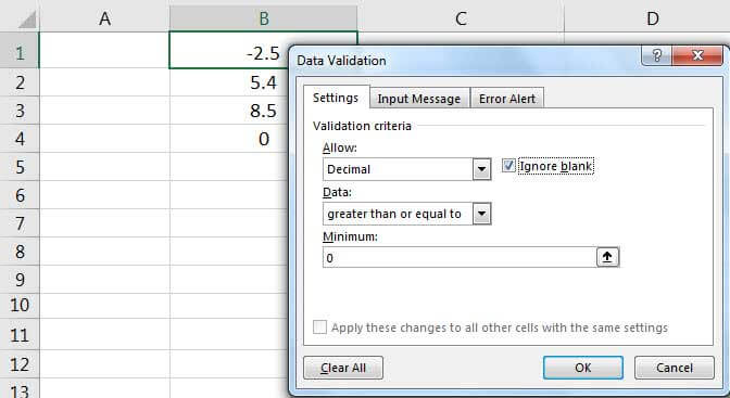
Step 2: The “data validation” window appears, as shown in the following image. In the “settings” tab, select “decimal” under the “allow” drop-down.

Under the “data” drop-down, select “greater than or equal to.” In the box under “minimum,” enter “0” (without the double quotation marks).

Step 3: In the “input message” tab, select the checkbox of “show input message when cell is selected.”

In the box under “title,” type “negative number detected” without the double quotation marks. In the box “input message,” type “enter number greater than zero.” This should also be written without the double quotation marks. Click “Ok.”

The data validation rule is created on cell B1. To cross-check it, select the validated cell B1. The defined input message appears, as shown in the following image.

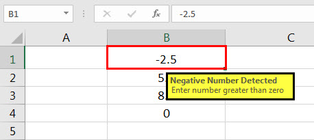
The number -2.5 was already there in cell B1 before the creation of the validation rule. This number is not deleted (from cell B1) even after creating a data validation rule.

However, in future, if a number is entered in cell B1, it must conform to the newly created rule. This implies that a decimal number greater than or equal to zero can be entered in cell B1. So, negative numbers are restricted in this cell. In case this rule is not complied with, Excel will display the default error alert.

Data Formats in Data validation

While entering data in a validated cell, there are certain formats that are allowed to the user. The rule creator (who is creating the data validation rule) can pick any of these formats based on which a validation rule can be created.

In the “settings” tab of the “data validation” window, the “allow” drop-down shows the following formats:

Any value: This implies that no validation will be executed. In case a data validation rule is created and then “any value” is selected, the created validation rule is removed. However, the input message of the created validation rule can be viewed even after “any value” has been selected.
Whole number: This requires that the user should enter a whole number in the validated cell.
Decimal: This implies that the data format allowed in the validated cell is decimal numbers.
List: This implies that the format allowed is a drop-down list. So, a drop-down list consisting of pre-defined values needs to be created. This drop-down list can be created in any of the following ways:
- Supply the values directly in the box under “source.”
- Provide the reference to the range (in the “source” box), which consists of the required values.
- Enter the name of the named range (in the “source” box), which begins with an “equal to” (=) sign.

Date: This implies that the user can enter only a date in the validated cell.
Time: This implies that a time value should be entered in the validated cell.
Text Length: This helps fix the number of digits or text entered in a validated cell. For instance, the user can enter either numbers or text up to 5 digits or 5 characters respectively.
Custom: This allows one to create a formula. This formula is used to validate (restrict) the input entered by the user. For instance, a formula can be entered to ensure that a text entry ends with certain characters, the text should be in uppercase or the entry must only be numeric, etc.

The Different Validation Criteria

Excel presents different criteria for validating data. The rule creator can select any of these criteria. Based on this selection, one can set the limits within which the input is allowed.

In the “settings” tab of the “data validation” dialog box, the drop-down under “data” shows the following validating criteria:

Between: This implies that the input should be between the minimum and the maximum numbers specified.
Not between: This implies that the input should not be between the minimum and the maximum numbers specified.
Equal to: This implies that the input should be equal to the specified value. In other words, the input should be the same as the specified value.
Not equal to: This implies that the input should not be equal to the specified value. In other words, the input should be different from the specified value.
Greater than: This implies that the input should be greater than the minimum number specified.
Less than: This implies that the input should be lesser than the maximum number specified.
Greater than or equal to: This implies that the input should be greater than or equal to the minimum number specified.
Less than or equal to: This implies that the input should be lesser than or equal to the maximum number specified.

The Different Error Alert Styles

There are different error alert styles in Excel. The rule creator can select any of these styles to notify the user that an error has been made while typing data in the validated cell.

In the “error alert” tab of the “data validation” window, the drop-down under “style” presents the following options:

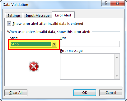
Stop: This stops the users from entering invalid data in the validated cell. With the “stop” style, the error alert message presents the following main options to the user:
- Retry– Clicking “retry” allows typing a new input.
- Cancel–Clicking “cancel” deletes the invalid input.

The “stop” style is the default error alert style of Excel.

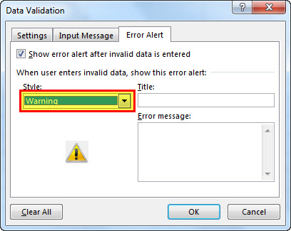
Warning: This warns the users that an invalid input has been entered. However, it does not stop the user from entering incorrect data. With the “warning” style, the user is presented with the following main options:
- Yes–Clicking “yes” makes Excel accept the invalid input.
- No–Clicking “no” allows typing a new input.
- Cancel–Clicking “cancel” deletes the invalid input.

Warning

Information: This informs the user that the input entered is invalid. Like the “warning” style, this also does not stop the user from entering incorrect data. With the “information” style, the user is presented with the following main options:
- Ok–Clicking “Ok” makes Excel accept the invalid input.
- Cancel–Clicking “cancel” deletes the invalid input.

By selecting a style, its respective icon appears in the error alert message displayed by Excel.

For instance, with the “stop” style, the cross within the red circle is shown (in the error alert message) as the user enters invalid data. Likewise, with the “warning” and “information” styles, the exclamation mark (within a yellow triangle) and the “i” sign (within a blue circle) show up respectively.

Note: Apart from the main options listed (in the preceding pointers 1, 2, and 3), Excel also displays the “help” option in all the error alert messages, irrespective of the style selected.

Purpose of Data Validation in Excel

The objectives of data validation in excel are listed as follows:

To restrict the users from entering unwanted or incorrect data values in the worksheet
To sort and study the data obtained with the help of defined criteria
To suggest the valid data format to the users through customized input messages (displayed when a validated cell is selected)

Excel Data validation is particularly helpful in the following situations:

When the number of users is large and there is a possibility of entering inputs in different formats
When the allowed entries need to be defined with a drop-down list
When an error alert (warning message) needs to be displayed on entering invalid data

The Limitations of Data Validation in Excel

The limitations of data validation in excel are listed as follows:

Data validation in excel does not prevent a user from copying an incorrect input from a non-validated cell to a validated cell. It can stop one from typing an incorrect input but not from copying the same. Hence, the purpose of data validation can become pointless if a user copies and pastes an invalid input.
Excel Data validation cannot fully protect a worksheet from invalid data entries. If a user copies an incorrect input from a non-validated cell and pastes it in a validated cell, the validation rule in the latter cell is eliminated. As a result, the validation rule is absent on the copied data.

Frequently Asked Questions

1. Define data validation in Excel.

Data validation restricts (limits) the type of input entered by a user in the worksheet. One can set the criteria for a specific cell and ensure that the input typed (in that cell) complies with it.

For instance, in cell A1, one is allowed to type only a decimal number between 1.5 and 9.5. This is a data validation rule applied to cell A1 of the worksheet.

2. How can a data validation rule be edited in Excel?

Let us say that rule X has been applied to cells A1 and D1. We want to change this to rule Y for both the mentioned cells.

The steps to edit a data validation rule are listed as follows:

a. Select any of the cells to which rule X has been applied.
b. Select “data validation” from the “data validation” drop-down (in the “data tools” group) of the Data tab.
c. In the “settings” tab of the “data validation” window, enter the new criteria as per rule Y.
d. Select the checkbox of “apply these changes to all other cells with the same settings.” This ensures that rule Y is applied to both the cells A1 and D1.
e. Click “Ok.”

The rule Y has been applied to both cells A1 and D1.

Note: The new data validation rule can be applied to all the validated cells only if they all had the same validation criteria initially. In this case, the initial validation criterion (rule X) was the same for both the validated cells (A1 and D1).

3. How can a data validation rule be removed in Excel?

The steps to remove (delete) a data validation rule are listed as follows:

a. Select the validated cell.
b. From the “data validation” drop-down (in the “data tools” group) of the Data tab, select “data validation.”
c. The “data validation” window opens. In the “settings” tab, click “clear all” appearing at the bottom left side.
d. Click “Ok.”

The validation rule will be cleared from the selected cell (selected in step a).

Note: To remove the same validation rule applied to multiple cells, select the checkbox of “apply these changes to all other cells with the same settings.” Thereafter, click “clear all” followed by “Ok.”

Try it!

Download our examples

Restrict data entry

Prompt users for valid entries

Display an error message when invalid data is entered

Add data validation to a cell or a range

Want more?

Introduction

Data validation controls

Important limitation

Defining data validation rules

Data validation options

Simple drop down menu

Data validation with a custom formula

Troubleshooting formulas

Data validation formula examples

Data validation to circle invalid entries

Find cells with data validation

Copy data validation from one cell to another

Clear all data validation

What is data validation in Excel with example?

How do you use data validation in Excel?

What is data validation used for?

What are the 3 types of data validation?

What is an example of validation?

What is Vlookup in Excel?

Why is data validation in Excel important?

What are the different types of validation?

What is data validation process?

What is validation method?

What are the 8 types of data validation rules?

What are validation rules?

What is the difference between data verification and data validation?

What is data validation in data analysis?

How do you validate survey data?

What is macro in Excel?

What is concatenate in Excel?

What is meant by pivot table?

What is Freeze Excel?

Data Validation:

Example of Data Validation

To use data validation as Date of Birth:

To use data validation as a List:

Table of contents

How to Use Data Validation in Excel?

Example #1–“Data Validation” Window Explained

Example #2–Decimal Number Validation

Data Formats in Data validation

The Different Validation Criteria

The Different Error Alert Styles

Purpose of Data Validation in Excel

The Limitations of Data Validation in Excel

Frequently Asked Questions

Recommended Articles