
A range is a group or block of cells in a worksheet that are selected or highlighted. Also, a range can be a group or block of cell references that are entered as an argument for a function, used to create a graph, or used to bookmark data.
Contents
- 1 What do you put for data range in Excel?
- 2 How do you define data range?
- 3 What is an example of a range in Excel?
- 4 How do you write a data range?
- 5 What is cell range explain with example?
- 6 Why is the range important?
- 7 What are the uses of range?
- 8 Where is define range option?
- 9 What is Range 7 Excel?
- 10 How do you show range in Excel?
- 11 What is range example?
- 12 What is maximum and minimum range?
- 13 What are the advantages of range in statistics?
- 14 What is a data range Google Sheets?
- 15 What is the synonym of range?
- 16 Which option is used to name a range of cell?
- 17 What is range in spreadsheet?
- 18 What is cell range Class 9?
- 19 What is name box?
- 20 How do you find the range?
What do you put for data range in Excel?
To select a data range, use the Go To feature as follows:
- Click any cell in the data range.
- Press [F5].
- In the Go To dialog, click the Special button in the bottom-left corner.
- In the resulting dialog, click the Current Region option.
- Click OK, and Excel will select the current data range (the current region).
How do you define data range?
In statistics, the range of a set of data is the difference between the largest and smallest values.
What is an example of a range in Excel?
A group of cells is known as a cell range. Rather than a single cell address, you will refer to a cell range using the cell addresses of the first and last cells in the cell range, separated by a colon. For example, a cell range that included cells A1, A2, A3, A4, and A5 would be written as A1:A5.
How do you write a data range?
Name a range
- Open a spreadsheet in Google Sheets.
- Select the cells you want to name.
- Click Data. Named ranges. A menu will open on the right.
- Type the range name you want.
- To change the range, click Spreadsheet .
- Select a range in the spreadsheet or type the new range into the text box, then click Ok.
- Click Done.
What is cell range explain with example?
When referring to a spreadsheet, the range or cell range is a group of cells within a row or column. For example, in the formula =sum(A1:A10), the cells in column A1 through A10 are the range of cells that are added together.For example, in the formula =sum(A1+B2+C3), the cells A1, B2, and C3 are added together.
Why is the range important?
How useful is the range? The range generally gives you a good indicator of variability when you have a distribution without extreme values. When paired with measures of central tendency, the range can tell you about the span of the distribution. But the range can be misleading when you have outliers in your data set.
What are the uses of range?
Range is typically used to characterize data spread. However, since it uses only two observations from the data, it is a poor measure of data dispersion, except when the sample size is large. Note that the range of Examples 1 and 2 earlier are both equal to 4.
Where is define range option?
Range option is available under d) Data menu.
Cell Range: A range is a group of contiguous cell, which form the shape of a rectangle. It can be group of two cell or as big as entire work sheet . For cell C1:C10 Indicates the range . Cell Reference And its Types:- The cell address that we use in the Formula is known as the cell reference.
How do you show range in Excel?
Find named ranges
- The Go to popup window shows named ranges on every worksheet in your workbook.
- To go to a range of unnamed cells, press Ctrl+G, enter the range in the Reference box, and then press Enter (or click OK).
What is range example?
The Range is the difference between the lowest and highest values. Example: In {4, 6, 9, 3, 7} the lowest value is 3, and the highest is 9. So the range is 9 − 3 = 6. It is that simple!
What is maximum and minimum range?
The largest value in a data set is often called the maximum (or max for short), and the smallest value is called the minimum (or min). The difference between the maximum and minimum value is sometimes called the range and is calculated by subtracting the smallest value from the largest value.
What are the advantages of range in statistics?
The range is the difference between the largest and the smallest observation in the data. The prime advantage of this measure of dispersion is that it is easy to calculate. On the other hand, it has lot of disadvantages. It is very sensitive to outliers and does not use all the observations in a data set.
What is a data range Google Sheets?
The “data range” is the set of cells you want to include in your chart. On your computer, open a spreadsheet in Google Sheets.Select the cells you want to include in your chart. Optional: To add more data to the chart, click Add another range. Then, select the cells you want to add.
What is the synonym of range?
Some common synonyms of range are compass, gamut, orbit, scope, and sweep. While all these words mean “the extent that lies within the powers of something (as to cover or control),” range is a general term indicating the extent of one’s perception or the extent of powers, capacities, or possibilities.
Which option is used to name a range of cell?
Using a named range
To use a named cell or range, click the down arrow in the Name box at the left end of the Formula bar. Select the range name you want to access, and Excel highlights the named cells. You can select a range name in the Name box to quickly locate an area of a worksheet.
What is range in spreadsheet?
A range is a group or block of cells in a worksheet that are selected or highlighted. Also, a range can be a group or block of cell references that are entered as an argument for a function, used to create a graph, or used to bookmark data.
What is cell range Class 9?
A cell range in Ms Excel is a collection of chosen cells. It can be referred to in a formula. This is defined in a spreadsheet with the reference of the upper-left cell as the minimum value of the range and the reference of the lower-right cell as the maximum value of the range.
What is name box?
Name Box is a tool that shows the active cell address. For example, if you have selected the cell C1, this name box will show the active cell address as C1.
How do you find the range?
The range is the simplest measurement of the difference between values in a data set. To find the range, simply subtract the lowest value from the greatest value, ignoring the others.
Find Range in Excel (Table of Contents)
- Range in Excel
- How to Find Range in Excel?
Range in Excel
Whenever we talk about the range in excel, it can be one cell or can be a collection of cells. It can be the adjacent cells or non-adjacent cells in the dataset.
What is Range in Excel & its Formula?
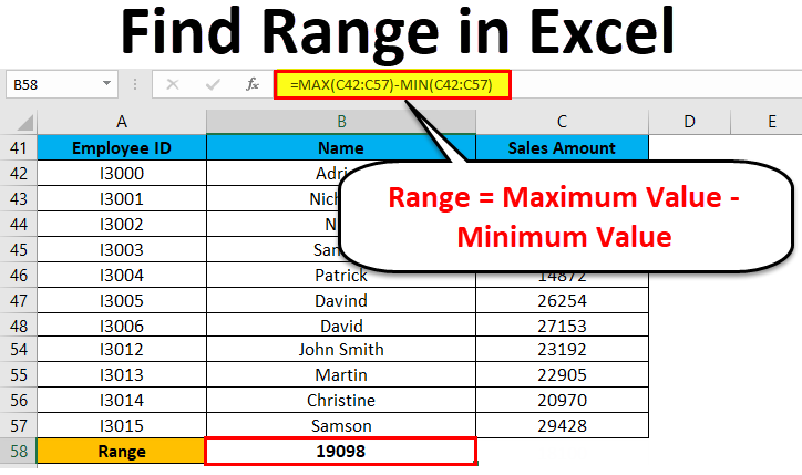
A range is the collection of values spread between the Maximum value and the Minimum value. A range is a difference between the Largest (maximum) value and the Shortest (minimum) value in a given dataset in mathematical terms.
Range defines the spread of values in any dataset. It calculates by a simple formula like below:
Range = Maximum Value – Minimum Value
How to Find Range in Excel?
Finding a range is a very simple process, and it is calculated using the Excel in-built functions MAX and MIN. Let’s understand the working of finding a range in excel with some examples.
You can download this Find Range Excel Template here – Find Range Excel Template
Range in Excel – Example #1
We have given below a list of values:
23, 11, 45, 21, 2, 60, 10, 35
The largest number in the above-given range is 60, and the smallest number is 2.
Thus, the Range = 60-2 = 58
Explanation:
- In this above example, the Range is 58 in the given dataset, which defines the span of the dataset. It gave you a visual indication of the range as we are looking for the highest and smallest point.
- If the dataset is large, it gives you the widespread of the result.
- If the dataset is small, it gives you a closely centered result.
A process of defining the range in Excel
For defining the range, we need to find out the maximum and minimum values of the dataset. In this process, two function plays a very important role. They are:
- MAX
- MIN
Use of MAX function:
Let’s take an example to understand the usage of this function.
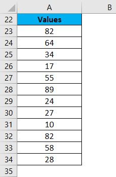
Range in Excel – Example #2
We have given some set of values:
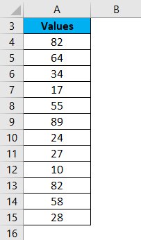
For finding the maximum value from the dataset, we will apply here the MAX function as below screenshot:
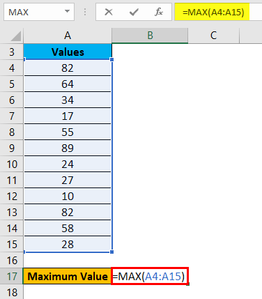
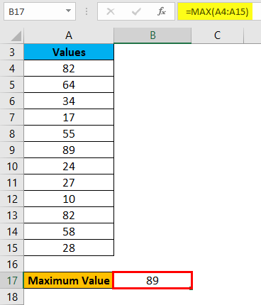
Hit enter, and it will give you the maximum value. The result is shown below:
Range in Excel – Example #3
Use of MIN function:
Let’s take the same above dataset to understand the usage of this function.
For calculating the minimum value from the given dataset, we will apply the MIN function here as per the below screenshot.
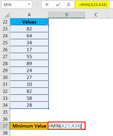
Press ENTER key, and it will give you the minimum value. The result is given below:
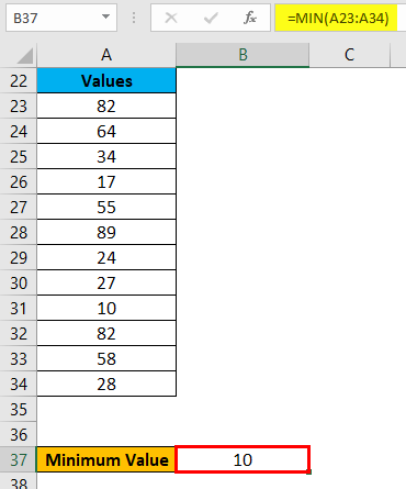
Now you can find out the range of the dataset after taking the difference between Maximum and Minimum value.
We can reduce the steps for calculating the range of a dataset by using the MAX and MIN functions together in one line.
For this, we again take an example to understand the process.
Range in Excel – Example #4
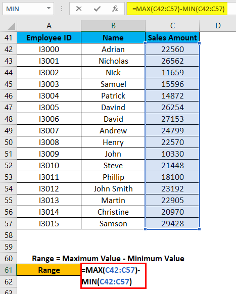
Let’s assume the below dataset of a company employee with their achieved sales target.
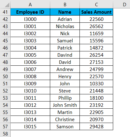
Now for identifying the span of sales amount in the above dataset, we will calculate the range. For this, we will follow the same procedure as we did in the above examples.
We will apply the MAX and MIN functions for calculating the Maximum and Minimum sales amount in the data.
For finding the range of sales amount, we will apply the below formula:
Range = Maximum Value – Minimum Value
Refer to the below screenshot:
Press Enter key, and it will give you the range of the dataset. The result is shown below:
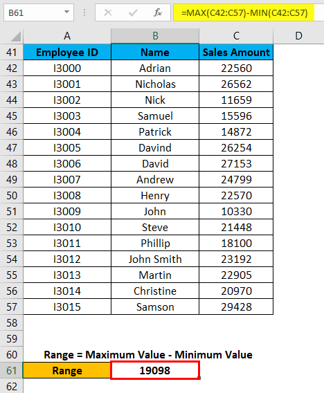
As we can see in the above screenshot, we applied the MAX and MIN formulas in one line, and by calculating their results difference, we found the range of the dataset.
Things to Remember
- If the values are available in the non-adjacent cells, you want to find out the range; you can pass the cell address individually, separated with a comma as an argument of the MAX and MIN functions.
- We can reduce the steps for calculating the range by applying MAX and MIN functions in one line. (Refer to Example 4 for your reference)
Recommended Articles
This has been a guide to Range in Excel. Here we discuss how to find Range in Excel along with excel examples and downloadable excel template. You may learn more about Excel from the following articles –
- Excel Function for Range
- Excel Named Range
- VBA Range
- VBA Selecting Range
A range is a group or block of cells in a worksheet that are selected or highlighted. Also, a range can be a group or block of cell references that are entered as an argument for a function, used to create a graph, or used to bookmark data.
The information in this article applies to Excel versions 2019, 2016, 2013, 2010, Excel Online, and Excel for Mac.
Contiguous and Non-Contiguous Ranges
A contiguous range of cells is a group of highlighted cells that are adjacent to each other, such as the range C1 to C5 shown in the image above.
A non-contiguous range consists of two or more separate blocks of cells. These blocks can be separated by rows or columns as shown by the ranges A1 to A5 and C1 to C5.
Both contiguous and non-contiguous ranges can include hundreds or even thousands of cells and span worksheets and workbooks.
Range Names
Ranges are so important in Excel and Google Spreadsheets that names can be given to specific ranges to make them easier to work with and reuse when referencing them in charts and formulas.
Select a Range in a Worksheet
When cells have been selected, they are surrounded by an outline or border. By default, this outline or border surrounds only one cell in a worksheet at a time, which is known as the active cell. Changes to a worksheet, such as data editing or formatting, affect the active cell.
When a range of more than one cell is selected, changes to the worksheet, with certain exceptions such as data entry and editing, affect all cells in the selected range.
There a number of ways to select a range in a worksheet. These include using the mouse, the keyboard, the name box, or a combination of the three.
To create a range consisting of adjacent cells, drag with the mouse or use a combination of the Shift and four arrow keys on the keyboard. To create ranges consisting of non-adjacent cells, use the mouse and keyboard or just the keyboard.
Select a Range for Use in a Formula or Chart
When entering a range of cell references as an argument for a function or when creating a chart, in addition to typing in the range manually, the range can also be selected using pointing.
Ranges are identified by the cell references or addresses of the cells in the upper left and lower right corners of the range. These two references are separated by a colon. The colon tells Excel to include all the cells between these start and endpoints.
Range vs. Array
At times the terms range and array seem to be used interchangeably for Excel and Google Sheets since both terms are related to the use of multiple cells in a workbook or file.
To be precise, the difference is because a range refers to the selection or identification of multiple cells (such as A1:A5) and an array refers to the values located in those cells (such as {1;2;5;4;3}).
Some functions, such as SUMPRODUCT and INDEX, take arrays as arguments. Other functions, such as SUMIF and COUNTIF, accept only ranges for arguments.
That’s not to say that a range of cell references cannot be entered as arguments for SUMPRODUCT and INDEX. These functions extract the values from the range and translate them into an array.
For example, the following formulas both return a result of 69 as shown in cells E1 and E2 in the image.
=SUMPRODUCT(A1:A5,C1:C5)
=SUMPRODUCT({1;2;5;4;3},{1;4;8;2;4})
On the other hand, SUMIF and COUNTIF do not accept arrays as arguments. So, while the formula below returns an answer of 3 (see cell E3 in the image), the same formula with an array would not be accepted.
COUNTIF(A1:A5,"<4")
As a result, the program displays a message box listing possible problems and corrections.
Thanks for letting us know!
Get the Latest Tech News Delivered Every Day
Subscribe
You are here
Working with data ranges in Excel
.
Excel is a powerful tool for manipulating large amounts of data. Make sure you know the rules Excel uses when setting up a data spreadsheet.
You can use Excel like a simple database to manage and manipulate large amounts of data. For example, you can sort a table of data based on the values in one or more columns. You can filter the same table to hide rows that don’t meet a set of criteria. You can insert subtotals and counts into the middle of a table of data based on criteria that you set. However, to get the most from Excel’s features you need to follow some simple rules.
Enter your data as a range
The first rule, and the most important, is to make sure your data is entered as a solid block of data, known as a table or range, that doesn’t contain any empty rows columns anywhere within the range. Excel uses empty columns and rows to determine where the edges of a range are. A lot of people like to insert empty rows and columns to space their data out. This might look good, but it stops your data from functioning correctly as a range. To test whether your data is correctly entered as a range, try clicking on one cell in the range and pressing the shortcut key combination CTRL+*. If you don’t have a number keyboard, press CTRL+SHIFT+8. This will select what Excel sees as the range. If it doesn’t select the right data, review your data for empty cells or rows.
All columns must have headings
The second rule is to ensure that your columns have a unique title at the top. Excel can usually manage without column headings, but your life will be a lot easier if you’ve got headings in your data table. A common mistake people make when entering columns is to split the heading into two rows so that the title fits neatly in to the column width they’ve defined. Problem is, Excel will treat the first row as the heading and the second row as part of the data. Use Excel’s Word Wrap feature instead to make long headings wrap within the cell.
.
Want to learn more? Try these lessons:
.
.
Our Comment Policy.
We welcome your comments and questions about this lesson. We don’t welcome spam. Our readers get a lot of value out of the comments and answers on our lessons and spam hurts that experience. Our spam filter is pretty good at stopping bots from posting spam, and our admins are quick to delete spam that does get through. We know that bots don’t read messages like this, but there are people out there who manually post spam. I repeat — we delete all spam, and if we see repeated posts from a given IP address, we’ll block the IP address. So don’t waste your time, or ours. One other point to note — if you post a link in your comment, it will automatically be deleted.
Add a comment to this lesson
.
.
.
.
There is a good amount of confusion around the terms ‘Table’ and ‘Range’, especially among new Excel users.
You will find many tutorials use the terms interchangeably too.
But the two terms have some basic differences that need to be identified.
In this tutorial, we will explain what the terms Table and Range / Named range mean, how to distinguish between them, as well as how you can convert from one form to the other in Excel.
Any group of selected cells can be considered as an Excel range.
A range of cells is defined by the reference of the cell that is at the upper left corner and the one at the lower right corner.
For example, the range selected in the image below consists of cells A1 to C7, denoted as A1:C7.

An Excel range does not require cells to be contiguous. You can also add cells to a range that are away from each other.
What is an Excel Named Range?
A named range is simply a range of cells with a name.
The main purpose of using named ranges is to make references to a group of cells more intuitive.
For example, if the name of the following selected range is “Sales”, then you can simply refer to this range by name in formulas (rather than using cell references like B2:B7):

To convert a range of cells to a named range, all you need to do is select the range, type the name into the Name Box and press the return key.

You can identify a named range by selecting the range of cells.
If you see a name, instead of a cell reference in the name box, then the range of cells belongs to a Named range.
What is an Excel Table?
An Excel Table is a dynamic range of cells that are pre-formatted and organized.
A table comes with some additional features such as data aggregation, automatic updates, data styling, etc.
You can say that an Excel table is basically an Excel range, but with some added functionality.
Like named ranges, Excel tables help group a set of related cells together, with a given name.
However, they also help users clearly see the grouping through some extra styling.
As Excel is releasing new data analysis features such as Power Query, Power Pivot, and Power BI, Excel Table has become even more important. Since it’s more structured, most of these new functionalities will require you to convert your data/range into an Excel Table.
How to Identify a Table in Excel?
You can easily identify a table in Excel thanks to its distinguishable features:
- You will find filter arrows next to each column header.

- Column headings remain frozen even as you scroll down the table rows.
- The table is enclosed in a distinguishable box.

- You will also find the table styled differently from the rest of the worksheet. For example you might find rows of the table styled in alternating colors for easy viewing.
- When you click on the table (or select any cell within the table), you should see a Design tab in the main menu.

- When you click on the Design tab, you should see the name of the table on the left side of the menu ribbon.

What’s the Difference Between an Excel Table and Range?
From the first glance, it is quite easy to differentiate between a table and a range.
Not only do they look different, they are also quite different in the amount of functionality they offer.
Here are some of the differences between an Excel Table and Range:
- Cells in an Excel table need to exist as a contiguous collection of cells. Cells in a range, however, don’t necessarily need to be contiguous.
- Every column in an Excel table must have a heading (even if you choose to turn the heading row of the table off). Named ranges, on the other hand, have no such compulsion.
- Each column header (if displayed) includes filter arrows by default. These let you filter or sort the table as required. To filter or sort a range, you need to explicitly turn the filter on.
- New rows added to the table remain a part of the table. However, new rows added to a range or are not implicitly part of the original range.
- In tables, you can easily add aggregation functions (like sum, average, etc.) for each column without the need to write any formulas. With ranges, you need to explicitly add whatever formulas you need to apply.

- In order to make formulas easier to read, cells in a table can be referenced using a shorthand (also known as a structured reference). This means that instead of specifying cell references in a formula (as in ranges), you can use a shorthand as follows:
=[@Qty]*[@Sales]

- Moreover, in a table, typing the formula for one row is enough. The formula gets automatically copied to the rest of the rows in the table. In a range or named range, however, you need to use the fill handle to copy a formula down to other rows in a column.
- Adding a new row to the bottom of a table automatically copies formulae to the new row. With ranges, however, you need to use the fill handle to copy the formula every time you insert a new row.
- Pivot tables and charts that are based on a table get automatically updated with the table. This is not the case with cell ranges.
How to Convert a Range to a Table
Converting an Excel range to a table is really easy.
Let’s say you have the following range of cells and you want to convert it to a table:

Here are the steps that you need to follow to convert the range into a table:
- Select the range or click on any cell in your range.
- From the Home tab, click on ‘Format as Table’ (under the Styles group).

- You should now see a dropdown menu with a number of styling options. Select the styling option that you want to apply to your table. We selected the option highlighted below:

- This will open the ‘Format as Table’ dialog box.
- Make sure that the range displayed under ‘where is the data for your table’ is correct.

- You should see a dashed box around the cells that will be part of your table.

- If your dataset has headers, ensure that the checkbox next to ‘My table has headers’ is checked.

- Click OK.
Here’s what your table should look like if you’ve followed the above steps:

Note: Alternatively, you could use the keyboard shortcut CTRL+T in place of steps 2 and 3.
How to Convert a Table to Range
It is also possible to reverse the conversion, in other words, convert a table back into a range of cells. Here are the steps that you need to follow:
- Select any cell in your table.
- You should see a new ribbon titled ‘Table Tools’ in the main menu. Select the Design tab under this menu.

- In the Tools group, select the ‘Convert to Range’ button.

- You will be asked to confirm if you want to convert the table to a normal range. Click Yes.

Alternatively, you could simply right-click on the table and select Table->Convert to Range from the context menu that appears.

You will now find that the table features (like filter arrows and structured references in all the formulas) are no longer there since it’s now just a regular range of cells. Structured references have all turned back into regular cell references.

In this tutorial, we explained with examples how ranges and named ranges differ from tables.
To conclude, a table can be considered as a named range, but with some added functionality, like styling, easy aggregations, structured references, and more.
We hope we have been successful in clearing any confusion you might have had about ranges, named ranges, and tables.
Other Excel Tutorials you may also like:
- How to Save an Excel Table as Image
- How to Add a Total Row in Excel Table
- How to Find Range in Excel
- SUMPRODUCT vs SUMIFS Function in Excel
- How to Paste in a Filtered Column Skipping the Hidden Cells
- How to Group by Months in Excel Pivot Table?
- How to Remove Table Formatting in Excel?
- How to Rename a Table in Excel?
- Row vs Column in Excel – What’s the Difference?