
A Data Model allows you to integrate data from multiple tables, effectively building a relational data source inside an Excel workbook. Within Excel, Data Models are used transparently, providing tabular data used in PivotTables and PivotCharts. A Data Model is visualized as a collection of tables in a Field List, and most of the time, you’ll never even know it’s there.
Before you can start working with the Data Model, you need to get some data. For that we’ll use the Get & Transform (Power Query) experience, so you might want to take a step back and watch a video, or follow our learning guide on Get & Transform and Power Pivot.
Where is Power Pivot?
-
Excel 2016 & Excel for Microsoft 365 — Power Pivot is included in the Ribbon.
-
Excel 2013 — Power Pivot is part of the Office Professional Plus edition of Excel 2013, but is not enabled by default. Learn more about starting the Power Pivot add-in for Excel 2013.
-
Excel 2010 — Download the Power Pivot add-in, then install the Power Pivot add-in.
Where is Get & Transform (Power Query)?
-
Excel 2016 & Excel for Microsoft 365 — Get & Transform (Power Query) has been integrated with Excel on the Data tab.
-
Excel 2013 — Power Query is an add-in that’s included with Excel, but needs to be activated. Go to File > Options > Add-Ins, then in the Manage drop-down at the bottom of the pane, select COM Add-Ins > Go. Check Microsoft Power Query for Excel, then OK to activate it. A Power Query tab will be added to the ribbon.
-
Excel 2010 — Download and install the Power Query add-in.. Once activated, a Power Query tab will be added to the ribbon.
Getting started
First, you need to get some data.
-
In Excel 2016, and Excel for Microsoft 365, use Data > Get & Transform Data > Get Data to import data from any number of external data sources, such as a text file, Excel workbook, website, Microsoft Access, SQL Server, or another relational database that contains multiple related tables.
In Excel 2013 and 2010, go to Power Query > Get External Data, and select your data source.
-
Excel prompts you to select a table. If you want to get multiple tables from the same data source, check the Enable selection of multiple tables option. When you select multiple tables, Excel automatically creates a Data Model for you.

-
Select one or more tables, then click Load.
If you need to edit the source data, you can choose the Edit option. For more details see: Introduction to the Query Editor (Power Query).
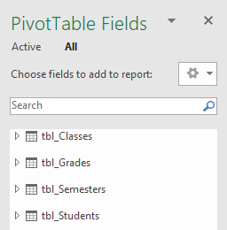
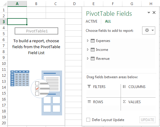
You now have a Data Model that contains all of the tables you imported, and they will be displayed in the PivotTable Field List.
Notes:
-
Models are created implicitly when you import two or more tables simultaneously in Excel.
-
Models are created explicitly when you use the Power Pivot add-in to import data. In the add-in, the model is represented in a tabbed layout similar to Excel, where each tab contains tabular data. See Get data using the Power Pivot add-into learn the basics of data import using a SQL Server database.
-
A model can contain a single table. To create a model based on just one table, select the table and click Add to Data Model in Power Pivot. You might do this if you want to use Power Pivot features, such as filtered datasets, calculated columns, calculated fields, KPIs, and hierarchies.
-
Table relationships can be created automatically if you import related tables that have primary and foreign key relationships. Excel can usually use the imported relationship information as the basis for table relationships in the Data Model.
-
For tips on how to reduce the size of a data model, see Create a memory-efficient Data Model using Excel and Power Pivot.
-
For further exploration, see Tutorial: Import Data into Excel, and Create a Data Model.
Create Relationships between your tables
The next step is to create relationships between your tables, so you can pull data from any of them. Each table needs to have a primary key, or unique field identifier, like Student ID, or Class number. The easiest way is to drag and drop those fields to connect them in Power Pivot’s Diagram View.
-
Go to Power Pivot > Manage.
-
On the Home tab, select Diagram View.
-
All of your imported tables will be displayed, and you might want to take some time to resize them depending on how many fields each one has.
-
Next, drag the primary key field from one table to the next. The following example is the Diagram View of our student tables:
We’ve created the following links:
-
tbl_Students | Student ID > tbl_Grades | Student ID
In other words, drag the Student ID field from the Students table to the Student ID field in the Grades table.
-
tbl_Semesters | Semester ID > tbl_Grades | Semester
-
tbl_Classes | Class Number > tbl_Grades | Class Number
Notes:
-
Field names don’t need to be the same in order to create a relationship, but they do need to be the same data type.
-
The connectors in the Diagram View have a «1» on one side, and an «*» on the other. This means that there is a one-to-many relationship between the tables, and that determines how the data is used in your PivotTables. See: Relationships between tables in a Data Model to learn more.
-
The connectors only indicate that there is a relationship between tables. They won’t actually show you which fields are linked to each other. To see the links, go to Power Pivot > Manage > Design > Relationships > Manage Relationships. In Excel, you can go to Data > Relationships.
-
Use a Data Model to create a PivotTable or PivotChart
An Excel workbook can contain only one Data Model, but that model can contain multiple tables which can be used repeatedly throughout the workbook. You can add more tables to an existing Data Model at any time.
-
In Power Pivot, go to Manage.
-
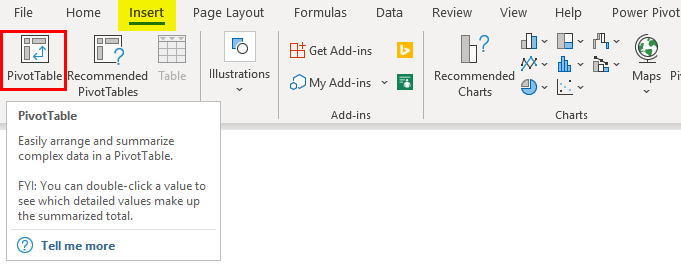
On the Home tab, select PivotTable.
-
Select where you want the PivotTable to be placed: a new worksheet, or the current location.
-
Click OK, and Excel will add an empty PivotTable with the Field List pane displayed on the right.
Next, create a PivotTable, or create a Pivot Chart. If you’ve already created relationships between the tables, you can use any of their fields in the PivotTable. We’ve already created relationships in the Student Data Model sample workbook.
Add existing, unrelated data to a Data Model
Suppose you’ve imported or copied lots of data that you want to use in a model, but haven’t added it to the Data Model. Pushing new data into a model is easier than you think.
-
Start by selecting any cell within the data that you want to add to the model. It can be any range of data, but data formatted as an Excel table is best.
-
Use one of these approaches to add your data:
-
Click Power Pivot > Add to Data Model.
-
Click Insert > PivotTable, and then check Add this data to the Data Model in the Create PivotTable dialog box.
The range or table is now added to the model as a linked table. To learn more about working with linked tables in a model, see Add Data by Using Excel Linked Tables in Power Pivot.
Adding data to a Power Pivot table
In Power Pivot, you cannot add a row to a table by directly typing in a new row like you can in an Excel worksheet. But you can add rows by copying and pasting, or updating the source data and refreshing the Power Pivot model.
Need more help?
You can always ask an expert in the Excel Tech Community or get support in the Answers community.
See Also
Get & Transform and Power Pivot learning guides
Introduction to the Query Editor (Power Query)
Create a memory-efficient Data Model using Excel and Power Pivot
Tutorial: Import Data into Excel, and Create a Data Model
Find out which data sources are used in a workbook data model
Relationships between tables in a Data Model
Содержание
- Создание модели данных в Excel
- Начало работы
- Создание связей между таблицами
- Создание сводной таблицы или сводной диаграммы с помощью модели данных
- Добавление имеющихся несвязанных данных в модель данных
- Добавление данных в таблицу Power Pivot данных
- Дополнительные сведения
- Create a Data Model in Excel
- Getting started
- Create Relationships between your tables
- Use a Data Model to create a PivotTable or PivotChart
- Add existing, unrelated data to a Data Model
- Adding data to a Power Pivot table
- Need more help?
Создание модели данных в Excel
Модель данных позволяет интегрировать данные из нескольких таблиц, эффективно создавая реляционный источник данных в книге Excel. В Excel модели данных используются прозрачно, предоставляя табличные данные, используемые в сводных таблицах и сводных диаграммах. Модель данных визуализируются как коллекция таблиц в списке полей, и в большинстве раз вы даже не узнаете, что она существует.
Прежде чем приступить к работе с моделью данных, необходимо получить некоторые данные. Для этого мы будем использовать интерфейс Get & Transform (Power Query), поэтому вам может потребоваться выполнить шаг назад и посмотреть видео, или следуйте нашему руководству по обучению по get & Transform и Power Pivot.
Excel 2016 & Excel для Microsoft 365 — Power Pivot включен в ленту.
Excel 2013 — Power Pivot входит в Office профессиональный плюс Excel 2013, но не включен по умолчанию. Дополнительные сведения о запуске надстройки Power Pivot для Excel 2013.
Excel 2010 — скачайте надстройку Power Pivot, а затем установите надстройку Power Pivot.
Excel 2016 & Excel для Microsoft 365 . Get & Transform (Power Query) интегрировано с Excel на вкладке «Данные«.
Excel 2013 — Power Query — это надстройка, которая входит в Excel, но ее необходимо активировать. Перейдите к разделу «Параметры >» > надстроек , а затем в раскрывающемся списке «Управление» в нижней части панели выберите com-надстройки > Go. Проверьте microsoft Power Query Excel, а затем ОК, чтобы активировать его. На Power Query будет добавлена вкладка Power Query.
Excel 2010 — скачивание и установка Power Query надстройки.. После активации на ленту Power Query вкладки.
Начало работы
Сначала необходимо получить некоторые данные.
В Excel 2016 и Excel для Microsoft 365 используйте data > Get & Transform Data > Get Data > Get Data to import data from any number of external data sources, such as a text file, Excel workbook, website, Microsoft Access, SQL Server, or another relational database that contains multiple related tables.
В Excel 2013 и 2010 перейдите к Power Query > получения внешних данных и выберите источник данных.
Excel предложит выбрать таблицу. Если вы хотите получить несколько таблиц из одного источника данных, установите флажок «Включить выбор нескольких таблиц «. При выборе нескольких таблиц Excel автоматически создает модель данных.
Примечание: В этих примерах мы используем книгу Excel с вымышленными сведениями о классах и оценках учащихся. Вы можете скачать пример книги модели данных учащихся и следовать инструкциям. Вы также можете скачать версию с готовой моделью данных..
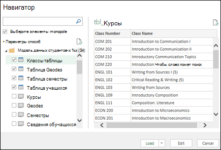
Выберите одну или несколько таблиц и нажмите кнопку «Загрузить «.
Если необходимо изменить исходные данные, можно выбрать параметр «Изменить «. Дополнительные сведения см. в статье «Общие сведения Редактор запросов (Power Query)».
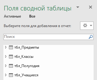
Теперь у вас есть модель данных, которая содержит все импортированные таблицы, и они будут отображаться в списке полей сводной таблицы.
Модели создаются неявно, когда вы импортируете в Excel несколько таблиц одновременно.
Модели создаются явно, если вы импортируете данные с помощью надстройки Power Pivot. В надстройке модель представлена в макете с вкладками, аналогичном Excel, где каждая вкладка содержит табличные данные. Дополнительные сведения об импорте данных с помощью надстройки Power Pivotсм. в статье «Получение данных с помощью SQL Server данных».
Модель может содержать одну таблицу. Чтобы создать модель на основе только одной таблицы, выберите таблицу и нажмите кнопку Добавить в модель данных в Power Pivot. Это может понадобиться в том случае, если вы хотите использовать функции Power Pivot, например отфильтрованные наборы данных, вычисляемые столбцы, вычисляемые поля, ключевые показатели эффективности и иерархии.
Связи между таблицами могут создаваться автоматически при импорте связанных таблиц, у которых есть связи по первичному и внешнему ключу. Excel обычно может использовать импортированные данные о связях в качестве основы для связей между таблицами в модели данных.
Советы по сокращению размера модели данных см. в статье «Создание модели данных, оптимизированной для памяти, с помощью Excel и Power Pivot».
Совет: Как определить, есть ли в книге модель данных? Перейдите Power Pivot > Управление. Если вы видите данные, как на листе, то модель существует. См. дополнительные сведения о том, какие источники данных используются в модели данных книги.
Создание связей между таблицами
Следующим шагом является создание связей между таблицами, чтобы вы могли извлекать данные из любой из них. Каждая таблица должна иметь первичный ключ или уникальный идентификатор поля, например идентификатор учащегося или номер класса. Самый простой способ — перетащить эти поля, чтобы подключить их в представлении схемы Power Pivot.
Перейдите в power Pivot > Manage.
На вкладке « Главная» выберите » Представление схемы».
Будут отображены все импортированные таблицы, и может потребоваться некоторое время, чтобы изменить их размер в зависимости от количества полей в каждой из них.
Затем перетащите поле первичного ключа из одной таблицы в следующую. В следующем примере показано представление схемы таблиц учащихся.
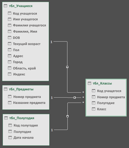
Мы создали следующие ссылки:
tbl_Students | Идентификатор учащегося > tbl_Grades | Идентификатор учащегося
Другими словами, перетащите поле «Идентификатор учащегося» из таблицы «Учащиеся» в поле «Идентификатор учащегося» в таблице «Оценки».
tbl_Semesters | Идентификаторы > tbl_Grades | Семестр
tbl_Classes | Номер класса > tbl_Grades | Номер класса
Имена полей не обязательно должны совпадать для создания связи, но они должны быть одинаковыми типами данных.
Соединители в представлении схемы имеют «1» с одной стороны, а «*» — с другой. Это означает, что между таблицами существует связь «один ко многим», которая определяет, как данные используются в сводных таблицах. См. дополнительные сведения о связях между таблицами в модели данных.
Соединители указывают только на наличие связи между таблицами. На самом деле они не показывают, какие поля связаны друг с другом. Чтобы просмотреть ссылки, перейдите в раздел Power Pivot > Manage > Design > Relationships > Управление связями. В Excel можно перейти к разделу «> данных».
Создание сводной таблицы или сводной диаграммы с помощью модели данных
Книга Excel может содержать только одну модель данных, но эта модель может содержать несколько таблиц, которые можно многократно использовать в книге. Вы можете добавить дополнительные таблицы в существующую модель данных в любое время.
В Power Pivotперейдите к разделу » Управление».
На вкладке « Главная» выберите сводную таблицу.
Выберите место размещения сводной таблицы: новый лист или текущее расположение.
Нажмите кнопку «ОК», и Excel добавит пустую сводную таблицу с областью списка полей справа.
Затем создайте сводную таблицу или сводную диаграмму. Если вы уже создали связи между таблицами, можно использовать любое из их полей в сводной таблице. Мы уже создали связи в образце книги модели данных учащихся.
Добавление имеющихся несвязанных данных в модель данных
Предположим, вы импортировали или скопировали много данных, которые вы хотите использовать в модели, но не добавили их в модель данных. Принудительно отправить новые данные в модель очень просто.
Начните с выбора любой ячейки в данных, которые необходимо добавить в модель. Это может быть любой диапазон данных, но лучше всего использовать данные, отформатированные в виде таблицы Excel .
Добавьте данные одним из следующих способов.
Щелкните Power Pivot > Добавить в модель данных.
Выберите Вставка > Сводная таблица и установите флажок Добавить эти данные в модель данных в диалоговом окне «Создание сводной таблицы».
Диапазон или таблица будут добавлены в модель как связанная таблица. Дополнительные сведения о работе со связанными таблицами в модели см. в статье Добавление данных с помощью связанных таблиц Excel в Power Pivot.
Добавление данных в таблицу Power Pivot данных
В Power Pivot невозможно добавить строку в таблицу, введя текст непосредственно в новой строке, как это можно сделать на листе Excel. Но можно добавить строки , скопируйте и вставьте или обновите исходные данные и обновите модель Power Pivot.
Дополнительные сведения
Вы всегда можете задать вопрос специалисту Excel Tech Community или попросить помощи в сообществе Answers community.
Источник
Create a Data Model in Excel
A Data Model allows you to integrate data from multiple tables, effectively building a relational data source inside an Excel workbook. Within Excel, Data Models are used transparently, providing tabular data used in PivotTables and PivotCharts. A Data Model is visualized as a collection of tables in a Field List, and most of the time, you’ll never even know it’s there.
Before you can start working with the Data Model, you need to get some data. For that we’ll use the Get & Transform (Power Query) experience, so you might want to take a step back and watch a video, or follow our learning guide on Get & Transform and Power Pivot.
Excel 2016 & Excel for Microsoft 365 — Power Pivot is included in the Ribbon.
Excel 2013 — Power Pivot is part of the Office Professional Plus edition of Excel 2013, but is not enabled by default. Learn more about starting the Power Pivot add-in for Excel 2013.
Excel 2016 & Excel for Microsoft 365 — Get & Transform (Power Query) has been integrated with Excel on the Data tab.
Excel 2013 — Power Query is an add-in that’s included with Excel, but needs to be activated. Go to File > Options > Add-Ins, then in the Manage drop-down at the bottom of the pane, select COM Add-Ins > Go. Check Microsoft Power Query for Excel, then OK to activate it. A Power Query tab will be added to the ribbon.
Excel 2010 — Download and install the Power Query add-in.. Once activated, a Power Query tab will be added to the ribbon.
Getting started
First, you need to get some data.
In Excel 2016, and Excel for Microsoft 365, use Data > Get & Transform Data > Get Data to import data from any number of external data sources, such as a text file, Excel workbook, website, Microsoft Access, SQL Server, or another relational database that contains multiple related tables.
In Excel 2013 and 2010, go to Power Query > Get External Data, and select your data source.
Excel prompts you to select a table. If you want to get multiple tables from the same data source, check the Enable selection of multiple tables option. When you select multiple tables, Excel automatically creates a Data Model for you.
Note: For these examples, we’re using an Excel workbook with fictional student details on classes and grades. You can download our Student Data Model sample workbook, and follow along. You can also download a version with a completed Data Model..

Select one or more tables, then click Load.
If you need to edit the source data, you can choose the Edit option. For more details see: Introduction to the Query Editor (Power Query).
You now have a Data Model that contains all of the tables you imported, and they will be displayed in the PivotTable Field List.
Models are created implicitly when you import two or more tables simultaneously in Excel.
Models are created explicitly when you use the Power Pivot add-in to import data. In the add-in, the model is represented in a tabbed layout similar to Excel, where each tab contains tabular data. See Get data using the Power Pivot add-into learn the basics of data import using a SQL Server database.
A model can contain a single table. To create a model based on just one table, select the table and click Add to Data Model in Power Pivot. You might do this if you want to use Power Pivot features, such as filtered datasets, calculated columns, calculated fields, KPIs, and hierarchies.
Table relationships can be created automatically if you import related tables that have primary and foreign key relationships. Excel can usually use the imported relationship information as the basis for table relationships in the Data Model.
For tips on how to reduce the size of a data model, see Create a memory-efficient Data Model using Excel and Power Pivot.
Tip: How can you tell if your workbook has a Data Model? Go to Power Pivot > Manage. If you see worksheet-like data, then a model exists. See: Find out which data sources are used in a workbook data model to learn more.
Create Relationships between your tables
The next step is to create relationships between your tables, so you can pull data from any of them. Each table needs to have a primary key, or unique field identifier, like Student ID, or Class number. The easiest way is to drag and drop those fields to connect them in Power Pivot’s Diagram View.
Go to Power Pivot > Manage.
On the Home tab, select Diagram View.
All of your imported tables will be displayed, and you might want to take some time to resize them depending on how many fields each one has.
Next, drag the primary key field from one table to the next. The following example is the Diagram View of our student tables:
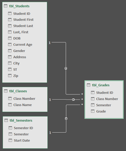
We’ve created the following links:
tbl_Students | Student ID > tbl_Grades | Student ID
In other words, drag the Student ID field from the Students table to the Student ID field in the Grades table.
tbl_Semesters | Semester ID > tbl_Grades | Semester
tbl_Classes | Class Number > tbl_Grades | Class Number
Field names don’t need to be the same in order to create a relationship, but they do need to be the same data type.
The connectors in the Diagram View have a «1» on one side, and an «*» on the other. This means that there is a one-to-many relationship between the tables, and that determines how the data is used in your PivotTables. See: Relationships between tables in a Data Model to learn more.
The connectors only indicate that there is a relationship between tables. They won’t actually show you which fields are linked to each other. To see the links, go to Power Pivot > Manage > Design > Relationships > Manage Relationships. In Excel, you can go to Data > Relationships.
Use a Data Model to create a PivotTable or PivotChart
An Excel workbook can contain only one Data Model, but that model can contain multiple tables which can be used repeatedly throughout the workbook. You can add more tables to an existing Data Model at any time.
In Power Pivot, go to Manage.
On the Home tab, select PivotTable.
Select where you want the PivotTable to be placed: a new worksheet, or the current location.
Click OK, and Excel will add an empty PivotTable with the Field List pane displayed on the right.
Next, create a PivotTable, or create a Pivot Chart. If you’ve already created relationships between the tables, you can use any of their fields in the PivotTable. We’ve already created relationships in the Student Data Model sample workbook.
Suppose you’ve imported or copied lots of data that you want to use in a model, but haven’t added it to the Data Model. Pushing new data into a model is easier than you think.
Start by selecting any cell within the data that you want to add to the model. It can be any range of data, but data formatted as an Excel table is best.
Use one of these approaches to add your data:
Click Power Pivot > Add to Data Model.
Click Insert > PivotTable, and then check Add this data to the Data Model in the Create PivotTable dialog box.
The range or table is now added to the model as a linked table. To learn more about working with linked tables in a model, see Add Data by Using Excel Linked Tables in Power Pivot.
Adding data to a Power Pivot table
In Power Pivot, you cannot add a row to a table by directly typing in a new row like you can in an Excel worksheet. But you can add rows by copying and pasting, or updating the source data and refreshing the Power Pivot model.
Need more help?
You can always ask an expert in the Excel Tech Community or get support in the Answers community.
Источник
What is the Data Model in Excel?
The data model in Excel is a type of data table where two or more two tables are in a relationship with each other through a common or more data series. In the data model, tables and data from various other sheets or sources come together to form a unique table that can access the data from all the tables.
For example, a data table containing tables of customers, product items, and product sellers. We can use the Excel data model to connect this dataset and create a relationship between them.
Table of contents
- What is the Data Model in Excel?
- Explanation
- Examples
- Example #1
- Example #2
- Things to Remember
- Recommended Articles
Explanation
- It allows integrating data from multiple tables by creating relationships based on a common column.
- Data models are used transparently, providing tabular data that can be used in a Pivot Table in ExcelA Pivot Table is an Excel tool that allows you to extract data in a preferred format (dashboard/reports) from large data sets contained within a worksheet. It can summarize, sort, group, and reorganize data, as well as execute other complex calculations on it.read more and Pivot Charts in excelIn Excel, a pivot chart is a built-in feature that allows you to summarize selected rows and columns of data in a spreadsheet. It is a visual representation of a pivot table that helps in the summarization and analysis of datasets, patterns, and trends.read more. In addition, it integrates the tables, enabling extensive analysis using pivot tables, power pivot, and Power View in ExcelExcel Power View is a data visualization technology that helps you create interactive visuals like graphs, charts. It allows you to analyze data by looking at the visuals you created. As a result, it makes your excel data more meaningful and insightful for better decision making.read more.
- The data model allows loading data into Excel’s memory.
- It is saved in memory, where we cannot directly see it. Then We can instruct Excel to relate data to each other using a common column. The ‘Model’ part of the data model refers to how all tables relate.
- The data model can access all the information it needs, even in multiple tables. After the data model is created, Excel has the data available in its memory. With the data in its memory, we can access the data in many ways.
You are free to use this image on your website, templates, etc, Please provide us with an attribution linkArticle Link to be Hyperlinked
For eg:
Source: Data Model in Excel (wallstreetmojo.com)
Examples
You can download this Data Model Excel Template here – Data Model Excel Template
Example #1
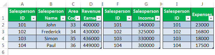
We have three datasets related to the salesperson: the first contains revenue information, the second includes the salesperson’s income and the third consists of the expenses of the salesperson.

To connect these three datasets and make a relationship with them, we make a data model with the following steps:
- Convert the datasets to table objects:
We cannot create a relationship with ordinary datasets. The data model works with only Excel TablesIn excel, tables are a range with data in rows and columns, and they expand when new data is inserted in the range in any new row or column in the table. To use a table, click on the table and select the data range.read more objects. To do this:
- Step 1 – We must first click anywhere inside the dataset, click on the “Insert” tab, and click on “Table” in the “Tables” group.
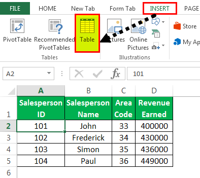
- Step 2 – Check or uncheck the ‘My table has headers’ option and click “OK.”
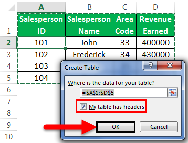
- Step 3 – We must enter the table’s name in the “Table Name” in the “Tools” group with the new table selected.
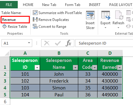
- Step 4 – Now, we can see that the first dataset is converted to a “Table” object. On repeating these steps for the other two datasets, we know that they also get converted to “Table” objects as below:
Adding the “Table” objects to the Data Model: Via Connections or Relationships.
Via Connections
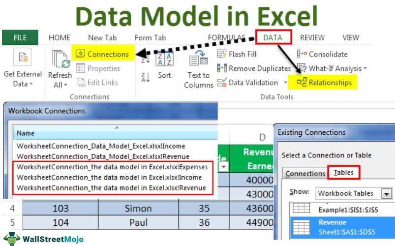
- We must select one table, click on the “Data” tab, and click on “Connections.”
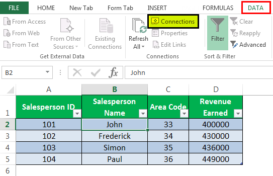
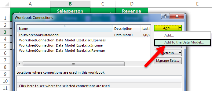
- There is an icon for “Add.” Expand the dropdown of “Add” and click on “Add to the Data Model” in the resulting dialog box.
- Click on “Tables” in the resulting dialog box, select one of the tables, and click “Open.”
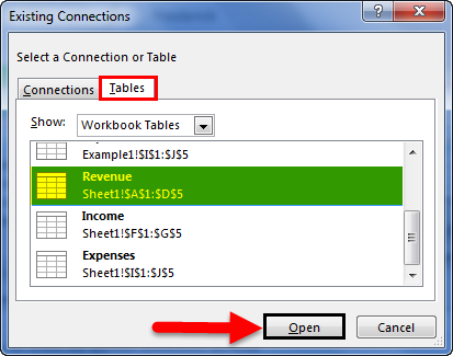
In doing this, it would create a workbook data model with one table, and a dialog box would appear as follows:
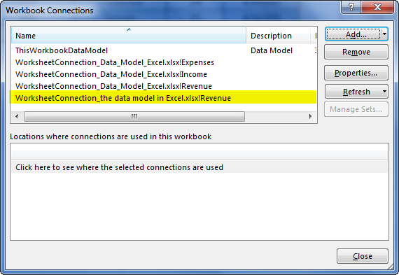
So if we repeat these steps for the other two tables, the data model will contain all three tables.
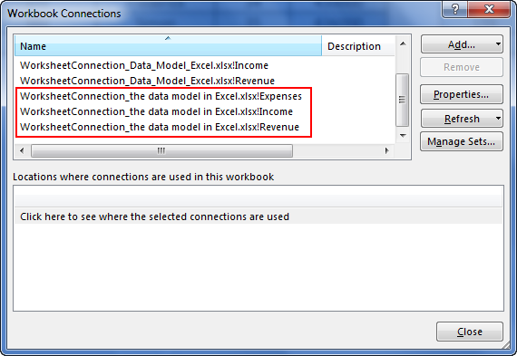
We can now see that all three tables appear in the “Workbook Connections.”
Via Relationships
Create the relationship: Once both the datasets are table objects, we can create a relationship between them. To do this:
- First, we should click on the “Data” tab and “Relationships.”
- As a result, we can see an empty dialog box with no current connections.
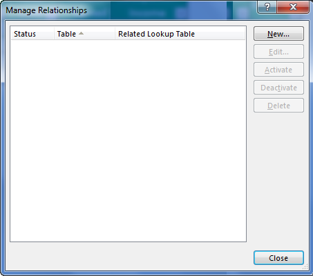
- Then, click on “New,” and another dialog box appears.
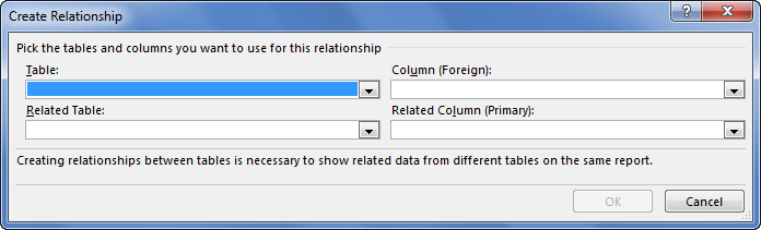
- Expand the “Table” and “Related Table” dropdowns: the “Create Relationship” dialog box appears to pick the tables and columns to use for a relationship. In the expansion of “Tables,” we must select the dataset we wish to analyze somehow, and in “Related Table,” we must choose the dataset with LOOKUP values.
- The lookup table in excelLookup tables are simply named tables that are used in combination with the VLOOKUP function to find any data in a large data set. We can select the table and name it, and then type the table’s name instead of the reference to look up the value.read more is the smaller table in the case of one to many relationships. It contains no repeated values in the common column. In expanding “Column (Foreign),” we must select the common column in the main table. In “Related Column (Primary),” we must choose the common column in the related table.
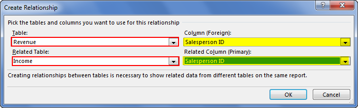
- With all these four settings selected, click on “OK.” A dialog box appears as follows on clicking on “OK.”
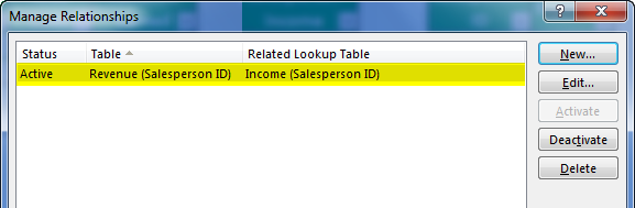
If we repeat these steps to relate the other two tables: the “Revenue” Table with “Expenses” table, then they also get connected in the data model as follows:
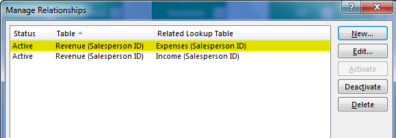
Excel now creates the relationship behind the scenes by combining data in the data model based on a common column: Salesperson ID (in this case).
Example #2
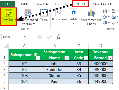
Now, in the above example, we wish to create a PivotTable that evaluates or analyzes the table objects:
- We must first click on “Insert” -> “PivotTable.”

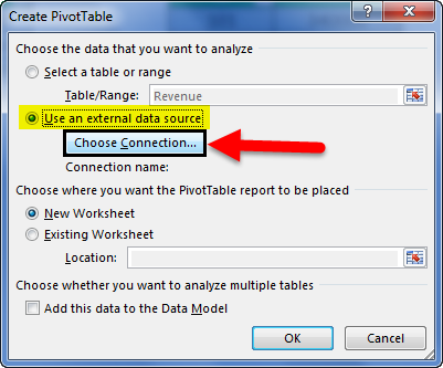
- We need to click on the “Use an external data source” option in the resulting dialog box and click on “Choose Connection.”

- Then, we must click on “Tables” in the resulting dialog box, select the “Workbook Data Model” containing three tables, and click “Open.”

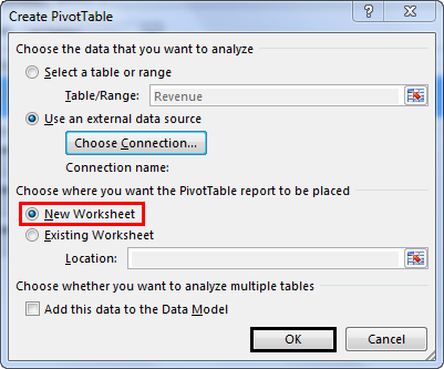
- Select the “New Worksheet” option in the location and click on “OK.”
- Consequently, the “PivotTable Fields” pane will display table objects.

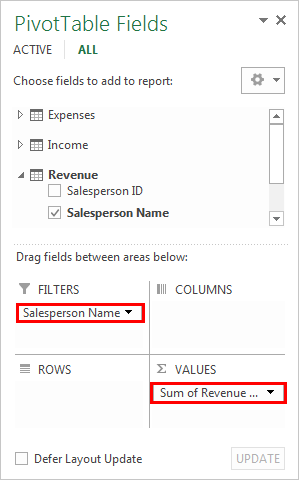
Now we can make changes in the PivotTable accordingly to analyze the table objects as required. - For instance, in this case, if we wish to find the total revenue or revenue for a particular salesperson, then a PivotTable is created as follows:


It is an immense help in the case of a model/table containing a large number of observations.


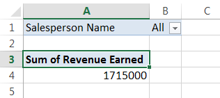
So, we can see that the pivot table instantly uses the data model (picking it by choosing connection) in Excel memory to show relationships between tables.
Things to Remember
- We can analyze data from several tables at once using the data model.
- By creating relationships with the data model, we surpass the need for using VLOOKUPThe VLOOKUP excel function searches for a particular value and returns a corresponding match based on a unique identifier. A unique identifier is uniquely associated with all the records of the database. For instance, employee ID, student roll number, customer contact number, seller email address, etc., are unique identifiers.
read more, SUMIF, INDEX functionThe INDEX function in Excel helps extract the value of a cell, which is within a specified array (range) and, at the intersection of the stated row and column numbers.read more, and MATCH formulas as we do not need to get all columns within a single table. - Models are implicitly created when datasets are imported in Excel from outside sources.
- We can create table relationships automatically if we import related tables with primary and foreign key relationships.
- While creating relationships, the columns that we are connecting in tables should have the same data type.
- With the pivot tables created with the data model, we can add slicers and slice them on any field at pivot tables we want.
- The advantage of the Data Model over LOOKUP() functionsThe LOOKUP excel function searches a value in a range (single row or single column) and returns a corresponding match from the same position of another range (single row or single column). The corresponding match is a piece of information associated with the value being searched.
read more is that it requires substantially less memory. - Excel 2013 supports only one-to-one or one to many relationships, i.e., one of the tables must have no duplicate values on the column we are linking to.
Recommended Articles
This article is a guide to Data Model in Excel. We discuss creating a data model from Excel tables using connections and relationships, practical examples, and a downloadable Excel template. You may learn more about Excel from the following articles: –
- Excel Value Formula
- Excel MATCH Formula
- Share an Excel Workbook
- Consolidate Data in Excel
Excel Data Model (Table of Contents)
- Introduction to Data Model in Excel
- How to Create a Data Model in Excel?
Introduction to Data Model in Excel
The data model feature of Excel enables the easy building of relationships between easy reporting and their background data sets. It makes data analysis much easier. It allows the integration of data from a plethora of tables spread across multiple worksheets by simply building relationships between matching columns. It works completely behind the scene and greatly simplifies reporting features such as PivotTable etc.
Our article shall attempt to show how to create a pivot table from two tables by employing the Data Model feature, thus establishing a relationship between two table objects and thereby creating a Pivot Table.
How to Create a Data Model in Excel?
Let’s understand how to create the Data Model in Excel with a few examples.
You can download this Data Model Excel Template here – Data Model Excel Template
Example #1
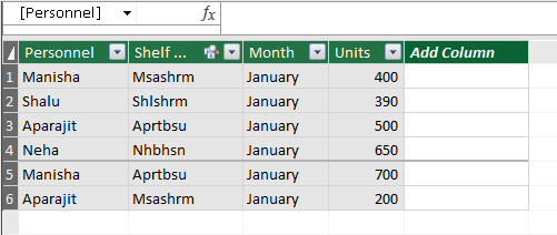
- We have a list of products, and we have a shelving code for each product. We need a table where we have the shelving description along with the shelving codes. So how do we incorporate the shelving descriptions against each shelving code? Perhaps many of us would resort to using VLOOKUP here, but we shall altogether remove the need to use VLOOKUP here using Excel Data Model.
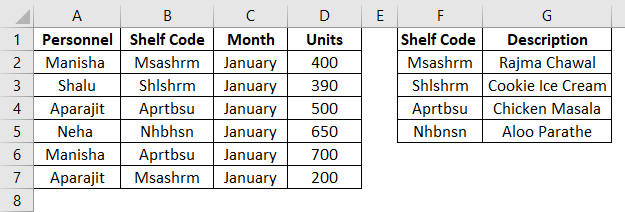
- The table on the left is the data table, and the table on the right is the lookup table. As we can see from the data, it is possible to create a relationship based on common columns.
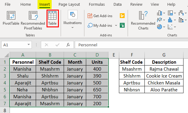
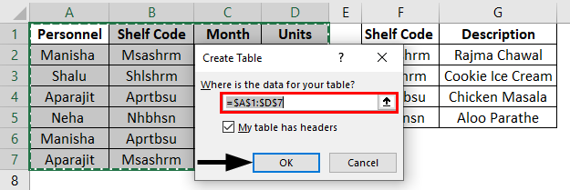
- Now, the Data Model is only compatible with table objects. So, it might be necessary sometimes to convert data sets to table objects. To do that, follow the below steps.
- Left-click anywhere in the data set.
- Click the Insert tab and navigate to Table in the Tables group or simply press Ctrl+T.
- Uncheck or check the My Table has the Header option. In our example, it does indeed have a header. Click OK.
- While still focused on the new table, we need to provide a name that is meaningful in the Name box (towards the left of the formula bar).
In our example, we have named the table Personnel.
- Now we need to do the same process for the lookup table as well and name it Shelf Code.
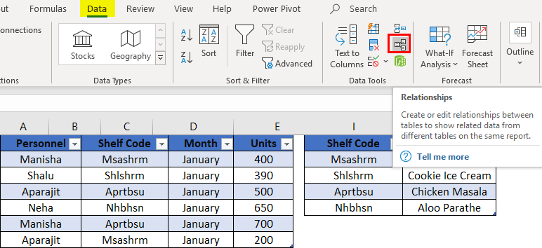
Creating a Relationship
So firstly, we shall go to the Data tab and then select Relationships in the Data Tools subgroup. After we click on the Relationships option, in the beginning, since there is no relationship, hence we will have nothing.
We will first click on New to create a relationship. We will now need to provide the primary and the lookup table names from the drop-down list and then also mention the column which is common between the two tables so that we can establish the relationship between the two tables from the drop-down list of columns.
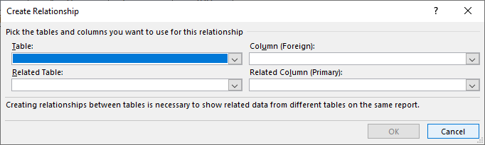
- Now, the primary table is the table that has the data. It is the primary data table – Table5. On the other hand, the Related table is the table that has the lookup data – it is our lookup table ShelfCodesTable. The primary table is the one that is analyzed based on the lookup table, which contains lookup data that will make the reported data, in the end, more meaningful.
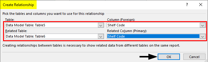
- So, the common column between the two tables is the Shelf Code column. This is what we have used to establish the relationship between the two tables. Coming to the columns, the Column (foreign) is the one that refers to the data table where there can be duplicate values. On the other hand, the Related Column (primary) refers to the column in the lookup table where we have unique values. We are simply setting up the field to lookup values from the lookup table in the data table.
- Once we set this up, Excel would create a relationship between the two behind the scene. It integrates the data and creates a data model based on the common column. This is light on the memory requirements and much faster than using VLOOKUP in large workbooks. After defining the Data model, Excel would be treating these objects as Data Model tables instead of a worksheet table.
- Now to see what Excel has been up to, we can click on Manage Data Models in Data -> Data Tools.
- We can also get the diagrammatic representation of the data model by changing the view. We will click on the View option. This will open up the view options. We will then select the Diagram View. Then we will see the diagrammatic representation, showing the two tables and the relationship between them, i.e. the common column – Shelf Code.
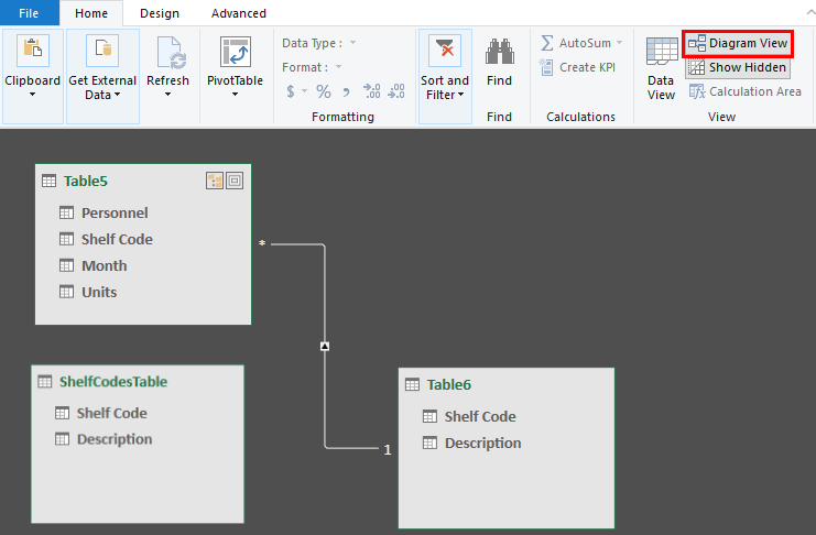
- The diagram above shows a one-to-many relationship between the unique lookup table values and the data table with duplicated values.
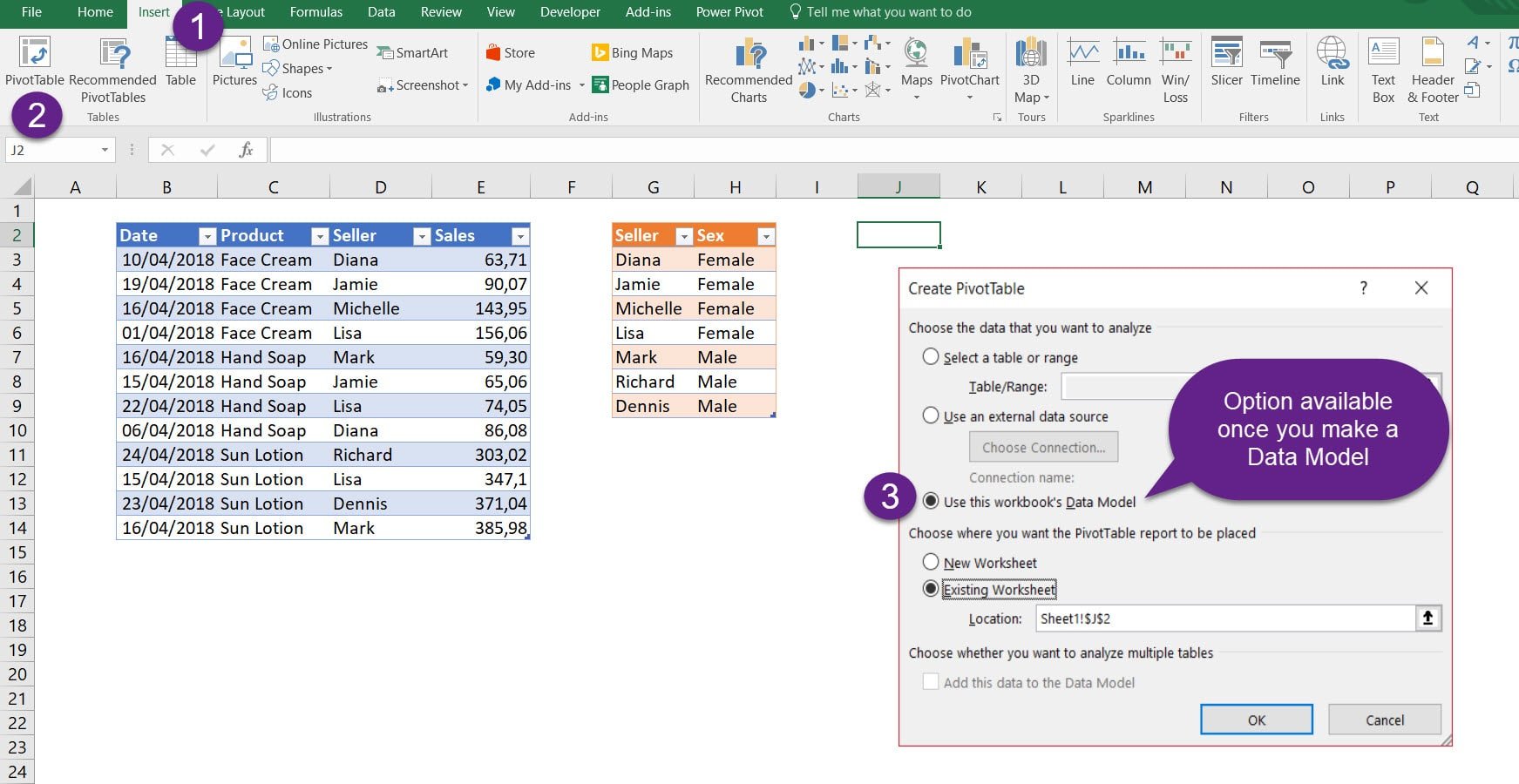
- Now we will have to create a pivot table. To do that, we will go to the Insert tab and then click on the Pivot Table option.
In the Pivot table’s Create Pivot Table dialogue box, we will select the source as “Use this workbook’s Data Model”.
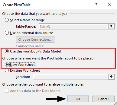
- This will create the Pivot table, and we can see that both the source tables are available in the source section.
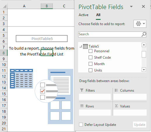
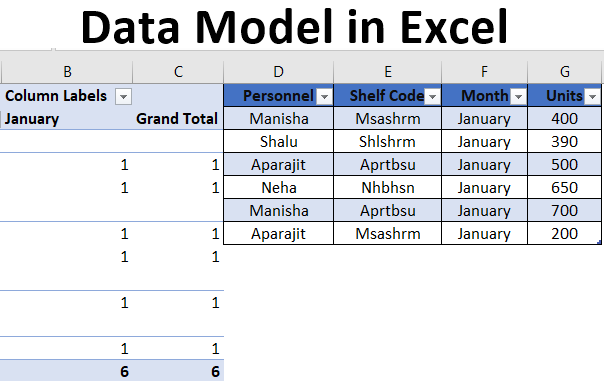
- Now we shall create a pivot table showing the count of each person who has shelved items.
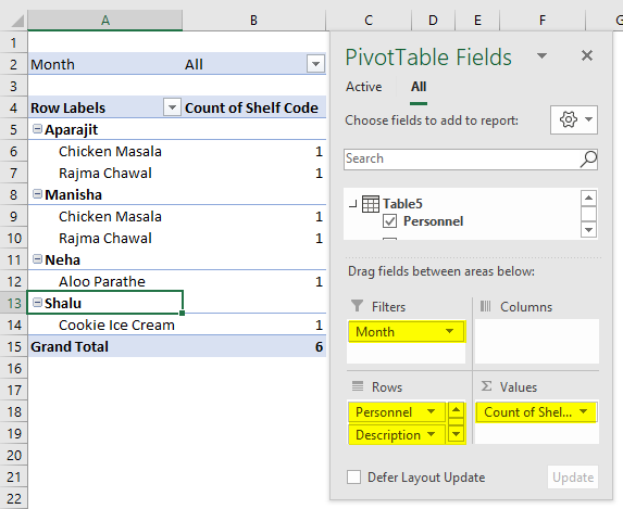
- We will select Personnel in the Rows section from Table 5 (data table), followed by Description (lookup table).
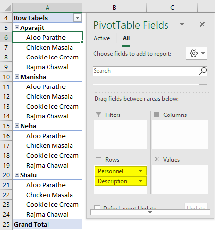
- Now we shall drag the Shelf Code from Table 5 into the Values section.
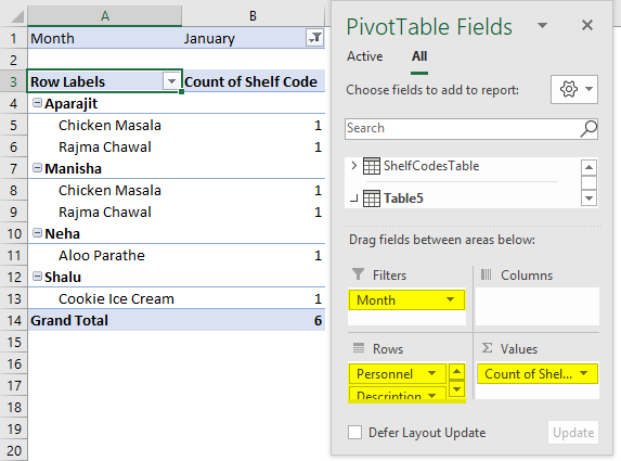
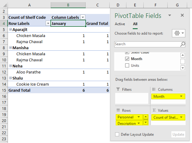
- Now we shall add Months from Table 5 to the Rows section.
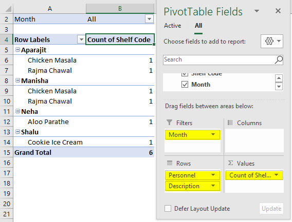
- Or we could add the months as a filter and add it to the Filters section.
Example #2
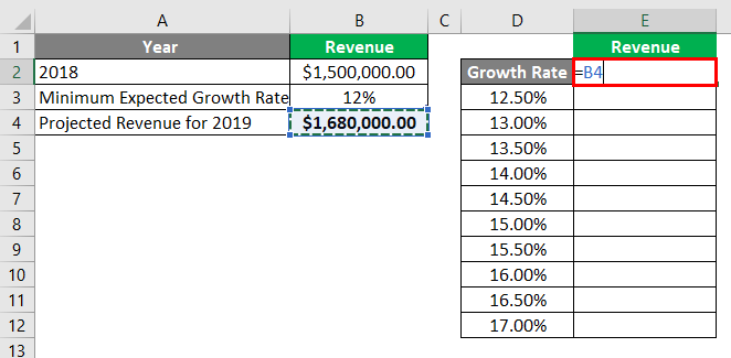
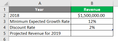
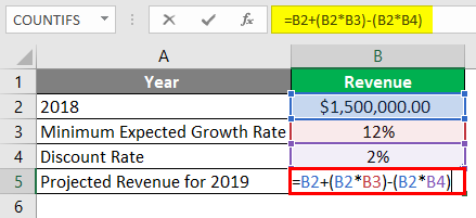
- We now have Mr Basu running a factory called Basu Corporation. Mr Basu is trying to estimate the revenue for 2019 based on the data from 2018.
- We have a table where we have the revenue for 2018 and the subsequent revenue at different incremental levels.
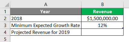
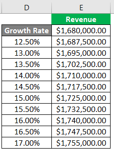
- So, we have the revenue for 2018 – $1.5 M, and the minimum growth expected the following year is 12%. Mr Basu wants a table that will show the revenue at different incremental levels.
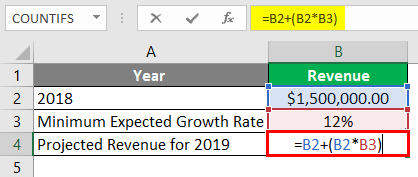
- We will create the following table for the projections at different incremental levels for 2019.
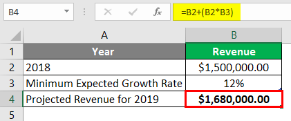
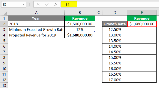
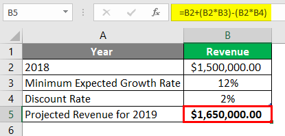
- Now we shall give the first Revenue row a reference to the estimated minimum revenue for 2019, i.e. $1.68 M.
- After using the formula, the answer is shown below.
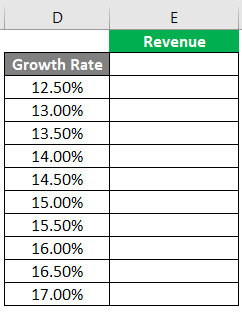
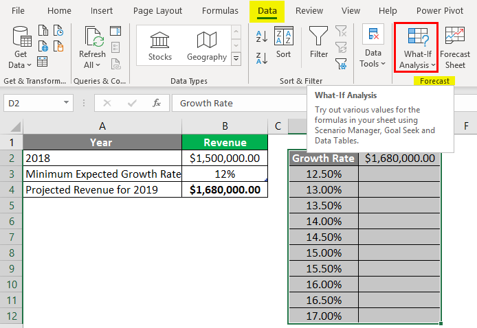
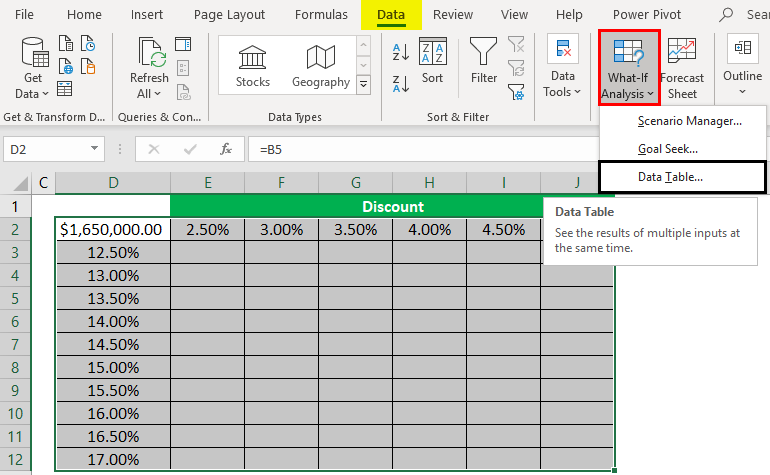
- Now we shall select the entire table, i.e. D2:E12 and then go to Data ->Forecast ->What-If Analysis ->Data Table.
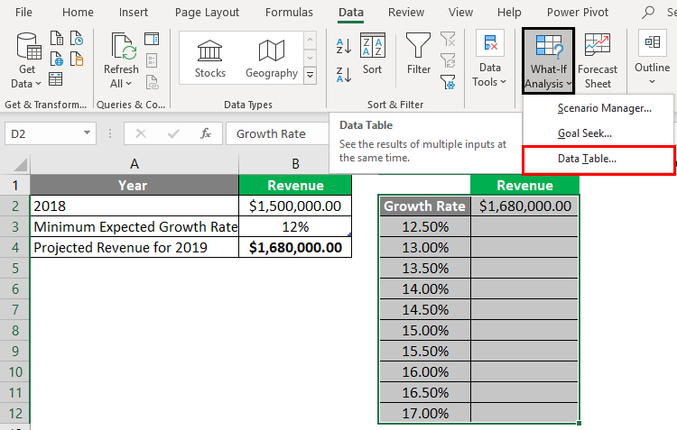
- This will open up the Data Table dialog box. Here we shall enter the minimum increment percent from cell B4 in the Column Input cell. The reason for that is that our projected estimated Growth percentages in the table are arranged in a columnar fashion.
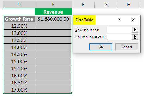
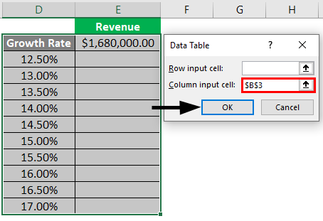
- Once we click OK, the What-If Analysis will automatically populate the table with projected revenue at the different incremental percentages.
Example #3
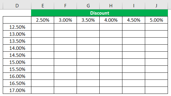
- Now suppose we have the same scenario as above, except that now we also have another axis to consider. Suppose, in addition to showing the projected revenue in 2019 based on the data of 2018 and the minimum expected growth rate, we now also have the estimated discount rate.
- First, we shall have a table shown below.
- Now we shall give reference to the minimum projected revenue for 2019, i.e. cell B5 to cell D8.
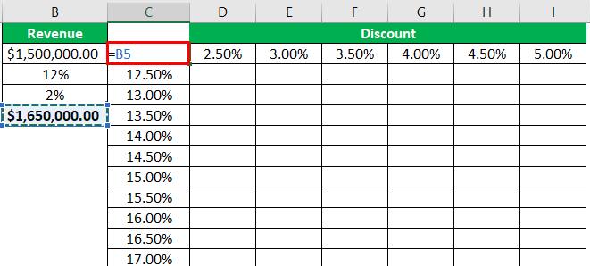
- Now we shall select the entire table, i.e. D8:J18 and then go to Data ->Forecast ->What-If Analysis ->Data Table.
- This will open up the Data Table dialog box. Here we shall enter the minimum increment percent from cell B3 in the Column Input cell. The reason for that is that our projected estimated Growth percentages in the table are arranged in a columnar fashion. We shall now also additionally enter the minimum discount percent from cell B4 in the Row Input cell. The reason for that is that our projected discount percentages in the table are arranged in a row-wise fashion.
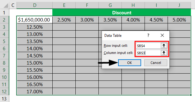
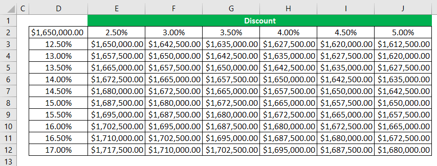
- Click OK. This will make the What-If Analysis automatically populate the table with projected revenue at the different incremental percentages as per the discount percentages.
Things to Remember About Data Model in Excel
- Upon successfully calculating the values from the data table, a simple Undo, i.e. Ctrl+Z, will not work. It is, however, possible to manually delete the values from the table.
- It is not possible to delete a single cell from the table. It is described as an array internally in Excel; hence we will have to delete all the values.
- We need to properly select the Row Input Cell and the Column Input Cell.
- The data table, unlike the Pivot Table, doesn’t need to be refreshed every time.
- Using the Data Model in Excel, we can improve performance and go easy on memory requirements in large worksheets.
- Data Models also makes our analysis much simpler as compared to using a number of complicated formulae all across the workbook.
Recommended Articles
This is a guide to Data Model in Excel. Here we discuss how to create Data Model in Excel along with practical examples and a downloadable excel template. You can also go through our other suggested articles –
- Pivot Table Slicer
- PowerPivot in Excel
- Pivot Table Formula in Excel
- Excel Pivot Table

Excel can analyze data from many sources. But are you using the Data Model to make your life easier? In this post you learn how to create a pivot table using two tables by using the Data Model feature in Excel.
What is a Data Model
Excel’s Data Model allows you to load data (e.g. tables) into Excel’s memory. It is saved in memory where you don’t directly see it. You can then instruct Excel to relate data to each other using a common column. The ‘Model’ part of Data Model refers to how all the tables relate to each other.
Old school Excel Pro’s, use formulas to create a huge table containing all data to analyze. They need this big table so that Pivot Tables can source a single table. Yet by creating relationships, you surpass the need for using VLOOKUP, SUMIF, INDEX-MATCH formulas. In other words, you don’t need to get all columns within a single table. Through relationships, the Data Model can access all the information it needs. Even when it resides in multiple places or tables. After creating the Data Model, Excel has the data available in its memory. And by having it in its memory, you can access data in new ways. For example, you can start using multiple tables within the same pivot table.
A Simple Task
Imagine your boss wants to have insight in the sales but also wants to know the Sex of the sales person. You got below dataset containing one table with the sales per person and another table containing the salespeople and their respective sex. A way to analyze your data is to use a LOOKUP formula and make a big table containing all information. As a next step you can then use a Pivot Table to summarize the data per sex.

Advantages of the Data Model
And before method is great when you work with very little data. Yet there are advantages of using the Data Model feature in Excel. Here follow some advantages:
- Checking and updating formulas may get arbitrary when working with many tables. After all, you need to make sure all the formulas are filled down to the right cell. And after adding new columns, your LOOKUP formulas also need to be expanded. The Data Model requires only little work at setup to relate a table. It uses a common column at the setup. Yet columns that you add later, automatically add to the Data Model.
- Working with big amounts of data often results in a very slow worksheet due to calculations. The Data Model however handles big amounts of data gracefully without slowing down your computer system.
- Excel 2016 has a limit of 1.048.576 rows. However, the amount of rows you can add to the memory of the Data Model is almost unlimited. A 64-bit environment imposes no hard limits on file size. The workbook size is limited only by available memory and system resources.
- If your data resides only in your Data Model, you have considerable file size savings.
Add Data to Data Model
You will now learn how to add tables to the Data Model. To start with, make sure your data is within a table. Using Power Query you can easily load tables into the Data Model.
- Click the Data tab -> Click a cell within the table you want to import
- Select From Table / Range

In the home tab of the Power Query editor
- Select Close & Load -> then Close & Load to…

- Select Only Create Connection
- Make sure to tick the box Add this data to the Data Model

This adds the data to the Data Model. Please make sure to do these steps for both tables.
Creating Relationships Between Data
After adding your data to the Data Model, you can relate common columns to each other. To create relationships between tables:
- Go to the tab Data -> Select Manage Data Model

The Power Pivot screen will appear.
- Click Diagram view. It gives you an overview of all the tables in the Data Model.
- Then relate the common column ‘Seller’ in the first table, with the column ‘Seller’ in the second table. You can do this by clicking-and-dragging one column, onto the other. A relationship should appear.

Note: When you make a relationship between 2 columns, it is common practice to have unique values in one of the columns. This is called a one-to-many relationship. Having duplicates on both sides may give you an error. For advanced calculations many-to-many relationships can exist (for example in Power BI). This however is too advanced to handle in this article. If you are interested in these topics make sure to research ‘Many-to-Many Relationships’.
Using the Data Model
Now we come to the exciting part. To use the Data Model in a PivotTable perform the following steps:
- Go to the tab Insert -> Click Pivot Table
The ‘Create PivotTable’ pop-up screen will appear. As you have a Data Model in place, you can now select to use it as data source.
- Click Use this workbook’s Data Model
In the PivotTable Fields you will now see all the possible Data Sources for your PivotTable. The yellow database icon on the lower right corner of the marked tables, shows that it is part of Excel’s Data Model.

As the two tables have a relationship between each other, you can use fields from both tables within the same pivot! Read previous sentence again. Isn’t that amazing?? Below example uses the Sales and Seller field from the ProductSales table, while the Sex field comes from the other table. And the numbers are still correct!

Conclusion
Using the Data Model you can analyze data from several tables at once. All without using any LOOKUP, SUMIF or INDEX MATCH formula to flatten the source table. Yet the data analyzed could also come from a database, text file or cloud location. The possibilities are endless.
To minimize the usage of LOOKUP formulas even more, an amazing tool to look at is Power Query. There’s several articles to find about it on my website. For example, you can read how to use Power Query for Creating Unique Combinations or for Transforming Stacked Columns.