
Table of Contents
- What is Excel Array?
- Excel Array Types
- Constant Array
- Array in Excel Range
- Array in Memory
- Name an array constant
What is Excel Array?
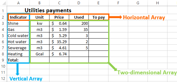
In Excel functions and formulas, an array is a collection of data elements in one row, one column, or multiple rows and columns. Array elements can be numeric, text, date, logical and error values.
The dimension of the array is the direction of the rows and columns of the array. An array with one row and multiple columns is a horizontal array, and an array with one column and multiple rows is a vertical array. An array with multiple rows and columns has both vertical and horizontal dimensions.
The dimensionality of an array is the number of different dimensions in the array. An array with only one row or column is called a one-dimensional array; an array with two dimensions with multiple rows and columns is called a two-dimensional array.
The size of an array is expressed by the number of elements in each row and column of the array.
- A
one-dimensional horizontal arraywith1rows andNcolumns has a size of1xN - A
one-dimensional vertical arraywith1column andNrows has a size ofNx1 - A
two-dimensional arraywithMrows andNcolumns has a size ofMxN
Excel Array Types
Constant Array
Constants arrays are string expressions that are written directly to the array elements in a formula and are identified by curly brackets “{}” at the beginning and end.
Constant arrays do not depend on the cell range, can be directly involved in the calculation of the formula.
Constant array elements can not be functions, formulas or cell references. Numeric constant elements can not contain dollar signs, commas and percent signs.
One-dimensional Array
The elements of a one-dimensional vertical array are separated by a colon “:“, the following is an array of numeric constants of size 5x1.
={10;20;30;40;50}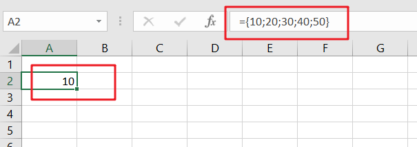
The elements of a one-dimensional horizontal array are separated by a comma “,”, and the following is an array of numeric constants of size 1×5:
={10,20,30,40,50}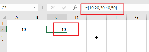
Note: For text-based constant arrays, each element in the array is identified by quotation marks by default.Two-dimensional Array
The elements of a two-dimensional array are separated by a semicolon “;” on each row and a comma “,” on each column.
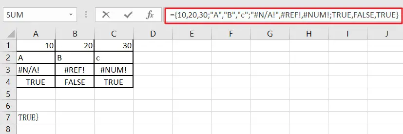
The following is a 4×3 two-dimensional array of mixed data types containing numeric, text, date, logical, and error values.
| 10 | 20 | 30 |
| A | B | c |
| #N/A! | #REF! | #NUM! |
| TRUE | FALSE | TRUE |
={10,20,30;"A","B","c";"#N/A!",#REF!,#NUM!;TRUE,FALSE,TRUE}
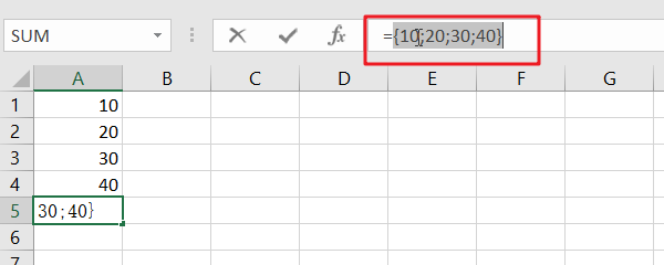
The process of manually entering a constant array can be tedious, you can use cell references to simplify the input of constant groups, the steps are as follows:
STEP1# Enter the value of the array element in the cell area, such as A1:A4
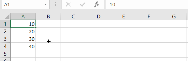
STEP2# Enter the formula =A1:A4 in cell A5
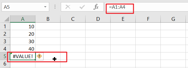
STEP3# In the formula bar, select the above formula and press F9, the formula can be converted to a constant array
Array in Excel Range
Range array is actually a formula directly referenced in the cell range, the size of the array and the size of the constant is exactly the same. For example, the following formulas A1:A4 and B1:B4 are range arrays.
=SUMPRODUCT (A1:A4*B1:B4)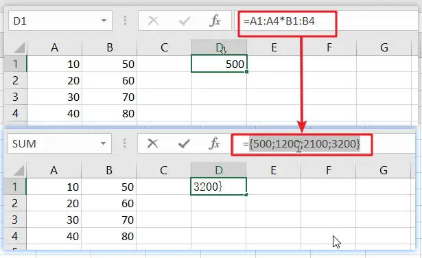
Array in Memory
A memory array is an array temporarily formed in memory by multiple values returned by a formula calculation. Memory arrays do not have to be stored in the cell range, and as a group can be directly nested in other formulas to continue to participate in the calculation. For example:
{ =SMALL(A1:A4,{1,2,3})}In the above formula, {1,2,3} is a constant group, and the entire formula results in a memory array of 1 row and 3 columns consisting of the smallest 3 numbers in the range of cells A1:A4.
Here is the array in memory.
={10,20,30}
The difference between memory array and area array:
- Range array is obtained by cell range reference, memory array is obtained by formula.
- Range Array depends on the referenced cell range, the memory array exists independently in memory.
Name an array constant
A named array is a constant array, a range array, or a memory array defined using a named formula (i.e., a name) that can be called as an array in a formula.

Note: You cannot use constant arrays directly in custom formulas used for data validation and conditional formatting, but you can use named arrays created through the Name Manager.bins_array – An array of intervals (“bins”) for grouping values.
Contents
- 1 What data array and bins array in Excel?
- 2 How do you split data into bins in Excel?
- 3 What is usage frequency?
- 4 What is frequency function?
- 5 How do I create a frequency distribution chart in Excel?
- 6 How does a Vlookup work?
- 7 What is bin array?
- 8 How do I figure out frequency?
- 9 What is a data bin?
- 10 What is bin width?
- 11 What is another word for frequency?
- 12 What are usage surveys?
- 13 What is frequency in survey?
- 14 How do you calculate frequency in Excel?
- 15 What is frequency distribution table?
- 16 How do you do a cumulative relative frequency graph in Excel?
- 17 Why is VLOOKUP so important?
- 18 How use VLOOKUP step by step?
- 19 What is VLOOKUP in simple words?
- 20 What does #spill mean in Excel?
FREQUENCY Function in Excel
- Data_array –It is an array or reference to a set of certain values whose frequencies we need to count.
- Bins_array–It is an array or reference to intervals into which you want to group the values in “data_array.”
How do you split data into bins in Excel?
On a worksheet, type the input data in one column, and the bin numbers in ascending order in another column. Click Data > Data Analysis > Histogram > OK. Under Input, select the input range (your data), then select the bin range.
What is usage frequency?
Usage Frequency is an at-a-glance metric that helps you determine how often an account is used. Totango looks at the past 14days of usage of an account and ranks their Usage Frequency into one of four possible values: Daily (9+ days from the last 14): Account is used almost every day.
What is frequency function?
The FREQUENCY function calculates how often values occur within a range of values, and then returns a vertical array of numbers. For example, use FREQUENCY to count the number of test scores that fall within ranges of scores. Because FREQUENCY returns an array, it must be entered as an array formula.
How do I create a frequency distribution chart in Excel?
Click here.
- Example Problem: Make a frequency distribution table in Excel.
- Step 1: Type your data into a worksheet.
- Step 2: Type the upper levels for your BINs into a separate column.
- Step 3: Make a column of labels so it’s clear what BINs the upper limits are labels for.
- Step 4: Click the “Data” tab.
How does a Vlookup work?
The VLOOKUP function performs a vertical lookup by searching for a value in the first column of a table and returning the value in the same row in the index_number position. The VLOOKUP function is a built-in function in Excel that is categorized as a Lookup/Reference Function.
What is bin array?
A vertical array of frequencies. =FREQUENCY (data_array, bins_array) data_array – An array of values for which you want to get frequencies. bins_array – An array of intervals (“bins”) for grouping values.
How do I figure out frequency?
To calculate frequency, divide the number of times the event occurs by the length of time. Example: Anna divides the number of website clicks (236) by the length of time (one hour, or 60 minutes). She finds that she receives 3.9 clicks per minute.
What is a data bin?
Data binning, also called discrete binning or bucketing, is a data pre-processing technique used to reduce the effects of minor observation errors. The original data values which fall into a given small interval, a bin, are replaced by a value representative of that interval, often the central value.
What is bin width?
A histogram displays numerical data by grouping data into “bins” of equal width. Each bin is plotted as a bar whose height corresponds to how many data points are in that bin. Bins are also sometimes called “intervals”, “classes”, or “buckets”.
What is another word for frequency?
What is another word for frequency?
| commonness | frequentness |
|---|---|
| prevalence | recurrence |
| repetition | constancy |
| amount | frequence |
| incidence | periodicity |
What are usage surveys?
It collected information and suggestions mainly about common standards, good practices, new features, new integrated services, and multilingualism.
What is frequency in survey?
A frequency distribution is a tabular representation of a survey data set used to organize and summarize the data. Specifically, it is a list of either qualitative or quantitative values that a variable takes in a data set and the associated number of times each value occurs (frequencies).
How do you calculate frequency in Excel?
Note: You also can use this formula =COUNTIF(A1:A10,”AAA-1″) to count the frequency of a specific value. A1:A10 is the data range, and AAA-1 is the value you want to count, you can change them as you need, and with this formula, you just need to press Enter key to get the result.
What is frequency distribution table?
A frequency distribution table is a chart that summarizes values and their frequency. It’s a useful way to organize data if you have a list of numbers that represent the frequency of a certain outcome in a sample. A frequency distribution table has two columns.
How do you do a cumulative relative frequency graph in Excel?
Example: Cumulative Frequency in Excel
To create the ogive chart, hold down CTRL and highlight columns A and C. Then go to the Charts group in the Insert tab and click the first chart type in Insert Column or Bar Chart: Along the top ribbon in Excel, go to the Insert tab, then the Charts group.
Why is VLOOKUP so important?
When you need to find information in a large spreadsheet, or you are always looking for the same kind of information, use the VLOOKUP function. VLOOKUP works a lot like a phone book, where you start with the piece of data you know, like someone’s name, in order to find out what you don’t know, like their phone number.
How use VLOOKUP step by step?
How to use VLOOKUP in Excel
- Step 1: Organize the data.
- Step 2: Tell the function what to lookup.
- Step 3: Tell the function where to look.
- Step 4: Tell Excel what column to output the data from.
- Step 5: Exact or approximate match.
What is VLOOKUP in simple words?
VLOOKUP stands for ‘Vertical Lookup‘. It is a function that makes Excel search for a certain value in a column (the so called ‘table array’), in order to return a value from a different column in the same row.
What does #spill mean in Excel?
#SPILL errors are returned when a formula returns multiple results, and Excel cannot return the results to the grid.
Содержание
- What is an array?
- Transcript
- Working with Excel array formula examples
- Types of Excel functions
- Array formulas syntax
- Working functions with Excel array
- Array
- Related terminology
- Example
- Array syntax
- Delimiters in other languages
- Arrays in formulas
- Array formulas
- Dynamic arrays
- Excel worksheet arrays and vectors
- 0. Arrays
- 1. Arrays — concepts
- Dimension
- Name Manager curly braces «<>«
- Function Arguments curly braces «<>«
- Formula F2 F9 curly braces «<>«
- 2. Arrays — element wise operators
- Example — Excel Online #1
What is an array?
Transcript
In this video, we’ll answer the question «what is an array?»
The term «array» comes from programming, but you’ll hear it come up often in the context of more advanced Excel formulas.
What does it really mean?
An array is a structure or container that holds a collection of items.
For example, this array contains 3 items, the numbers 10, 20, and 30:
And this array contains three text strings:
Note that arrays in Excel are always enclosed in curly braces.
The reason arrays come up so often in Excel formulas is that arrays can be mapped directly to ranges.
Arrays can be vertical, horizontal, or two-dimensional.
Vertical arrays have items separated with semicolons.
Horizontal arrays use commas.
Two-dimensional arrays use both commas and semicolons.
In this worksheet, we can represent the values in the range B6:B10 in an array like this:
Notice there are 5 cells in the range, and 5 items in the array.
The range D8:F8 can be represented in an array like this:
the range H5:I7 corresponds to a 2D array like this:
You can inspect arrays in a formula by using the F9 key. For example, if I start a formula with:
I can then use the F9 key to see the array that corresponds to this range.
In fact, if I copy this array to the clipboard, then start another formula and then paste, you can see that Excel understands how to map the items in the array to individual cells.
If I change a value manually, the corresponding cell updates.
Arrays like this — where all values are hardcoded — are called «array constants».
Array constants are useful in many formulas, and we’ll see more examples later on in the course.
Источник
Working with Excel array formula examples
The array of Excel functions allows you to solve complex tasks in automatically at the same time. We cannot complete the same tasks through the usual functions.
In fact, this is a group of functions that simultaneously process a group of data and immediately produce a result. Let’s consider in detail work with arrays of functions in Excel.
Types of Excel functions
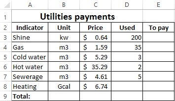
Array is a data grouped together. In this case, the group is an array of functions in Excel. Any table that we compose and fill in Excel can be called an array. Example:
Depending on the location of the elements, the arrays are distinguished:
- One-dimensional (data is in ONE line or in ONE column);
- Two-dimensional (SEVERAL lines and columns, matrix).
One-dimensional arrays are:
- Horizontal (data in a row);
- Vertical (data in a column).
Note. Two-dimensional Excel arrays can take several sheets at once (these are hundreds and thousands of data).
Array formula allows you to process data from this array. It can return one value or result in an array (set) of values.
With the help of array formulas it is real to:
- Count the number of characters in a certain range;
- Summarize only those numbers that correspond to the given condition;
- Summarize all n values in a certain range.
When we use array formulas, Excel takes into account the range of values not as individual cells, but as a single data block.
Array formulas syntax
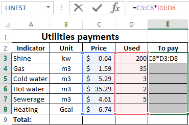
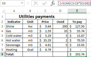
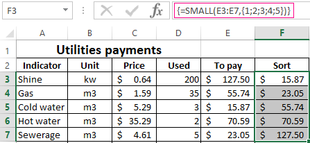
We use the formula of an array with a range of cells and with a separate cell. In the first case, we find the subtotals for the «To pay» «» column. In the second — the total amount of utility payments.
- We select the range E3: E8.
- Enter the following formula in the formula row: = C3: C8 * D3: D8.

- Press the keys simultaneously: Ctrl + Shift + Enter. The subtotals are calculated:
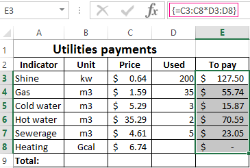
The formula after pressing Ctrl + Shift + Enter was in curly brackets. It was automatically inserted into each cell of the selected range.
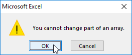
If you try to change the data in any cell in the «To pay» column, nothing happens. The formula in the array protects range values from changes. A corresponding entry appears on the screen:
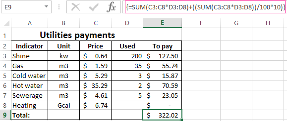
Consider other examples of using the functions of an Excel array — calculate the total amount of utility payments using a single formula.
- Select the cell E9 (opposite the «Total»).
- We introduce a formula of the form:
- Press the key combination: Ctrl + Shift + Enter. Result:
The formula of the array in this case replaced two simple formulas. This is a shortened version, which contains all the necessary information for solving a complex problem.
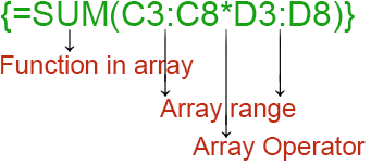
Arguments for a function are one-dimensional arrays. The formula looks at each of them individually, performs user-defined operations, and generates a single result.
Consider the syntax:
Working functions with Excel array
Let’s guess that it is planned to increase utility payments in 10% the next month. If we introduce the usual formula for the total is =SUM((C3:C8*D3:D8)+10%), then we are unlikely to get the expected result. We need each argument to increase in 10%. For the program to understand this, we use the function as an array.
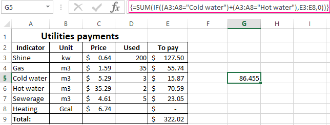
- Let’s have a look how the «И» «AND» operator works in the array function. We need to find out how much we pay for the water, hot and cold. Function: The total is 86.46$.
- The Sort functions in the array formula. Sort the amounts to be paid in ascending order. For the sorted data list, create a range. Let’s select it (F3:F7). In the formula bar, we enter Press Ctrl + Shift + Enter.
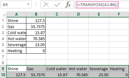
- The transported matrix. There is a special Excel function for working with two-dimensional arrays. The «ТРАНСП» function returns several values at once. It converts a horizontal matrix to a vertical matrix and vice versa. Select the range of cells where the number of rows equals to the number of columns in the table with the original data. And the number of columns equals to the number of rows in the source array. Select range A9:F10. We introduce the formula: Press Ctrl + Shift + Enter. This results in an «inverted» data set.
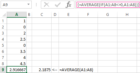
- Search for the average without taking into account zeros. If we use the standard «AVERAGE» function, we get «0» as a result. And it will be correct. Therefore, we insert an additional condition into the formula:
0,A1:A8))’ >
A common mistake when working with arrays of functions is NOT to press the code combination «Ctrl + Shift + Enter» (never forget this key combination). This is the most important thing to remember when processing large amounts of information. Correctly entered function performs the most complicated tasks.
Источник
Array

An array in Excel is a structure that holds a collection of values. Arrays can be mapped perfectly to ranges in a spreadsheet, which is why they are so important in Excel. An array can be thought of as a row of values, a column of values, or a combination of rows and columns with values. All cell references like A1:A5 and C1:F5 have underlying arrays, though the array structure is invisible in most contexts.
Example
In the example above, the three ranges map to arrays in a «row by column» scheme like this:
If we display the values in these ranges as arrays, we have:
Notice arrays must represent a rectangular structure.
Array syntax
All arrays in Excel are wrapped in curly brackets <> and the delimiters between array elements indicate rows and/or columns. In the US version of Excel, a comma (,) separates columns and a semicolon (;) separates rows. For example, both arrays below contain numbers 1-3, but one is horizontal and one is vertical:
Text values in an array appear in double quotes («») like this:
To «see» the array associated with a range, start a formula with an equal sign (=) and select the range. Then use the F9 key to inspect the underlying array. You can also use the ARRAYTOTEXT function to show how columns and rows are represented. Set format to 1 (strict) to see the complete array.
Delimiters in other languages
In other language versions of Excel, the delimiters for rows and column can vary. For example, the Spanish version of Excel uses a backslash () for columns and a semicolon (;) for rows:
Arrays in formulas
Since arrays map directly to ranges, all formulas work with arrays in some way, though it isn’t always obvious. A simple example is a formula that uses the SUM function to sum the range A1:A5, which contains 10,15,20,25,30. Inside SUM, the range resolves to an array of values. SUM then sums all values in the array and returns a single result of 100:
Note: you can use the F9 key to «see» arrays in your Excel formulas. See this video for a demo on using F9 to debug.
Array formulas
Array formulas involve an operation that delivers an array of results. For example, here is a simple array formula that returns the total count of characters in the range A1:A5:
Inside the LEN function, A1:A5 is expanded to an array of values. The LEN function then generates a character count for each value and returns an array of 5 results. The SUM function then returns the sum of all items in the array.
Dynamic arrays
With the introduction of Dynamic Array formulas in Excel, arrays have become more important, since it is easier than ever to write formulas that work with multiple results at the same time.
Источник
Excel worksheet arrays and vectors
This material about arrays and vectors involves three concepts:
- Excel structures able to hold data, most commonly, the array of cells on a worksheet (by reference, name or constant)
- mathematical element wise array operations, and
- matrix based linear algebra array operations
0. Arrays
An array can be described as a group of items that can be acted on either individually or collectively. An array’s orientation is classified by its dimension (such as column orientation, or row orientation, discussed further in section 1). In Excel the concept is best illustrated by example, see figure 1 (worksheet: WS arrays) where «a group of items» means a contiguous range, In particular, an array can be a:
- Scalar — a single cell
- Column array (column vector) — range B2:B7 shaded green
- Row array (row vector) — range B9:E9 shaded blue
- Multi dimensional array — range B11:D14 shaded grey
The expressions «scalar», «row vector» and «column vector» are common to the MatLab (matrix laboratory) application software.
 Fig 1: Column, Row and MultiDimensional array — CollArr (6R x 1C), RowArr (1R x 4C), and MDArr (4R x 3C) 12 elements
1. Arrays — concepts
Dimension
The size of an array is described by the number of rows and number of columns. By convention the dimension is always rows first and columns second, in the spirit of R1C1 reference style, and the ordering of row and column arguments in functions such as INDEX and OFFSET.
Excel uses [mR x nR] during selection resizing operations (m and n are common to MatLab). MatLab uses m x n notation, with m being the number of rows (first dimension) and n being the number of columns (second dimension). Thus [2R x 3C] is a 2 row by 3 column array.
An array is contiguous, meaning rectangular / square, and a worksheet array can be referenced by the top left cell and bottom right cell with the range operator, see B11:DF14 in figure 1. Some functions return an array (eg. the TRANSPOSE and MMULT functions).
Dimensions (from figure 1):
- Scalar: dimension 1 x 1 (not shown in figure)
- Column vector: named ColArr , dimension 6 x 1, number of elements 6
- Row vector: named RowArr , dimension 1 x 4, number of elements 4
- MultiDimensional array: a two dimensional array named MDArr , dimension 4 x 3, number of elements 12
In mathematics, the arrays in figure 1 can presented in the form:
$$text=begin r1 \ r2 \ r3 \ r4 \ r5 \ r6 end, qquad text=begin c1 & c2 & c3 & c4 end qquad text=begin r1c1 & r1c2 & r1c3 \ r2c1 & r2c2 & r2c3 \ r3c1 & r3c2 & r3c3 \ r4c1 & r4c2 & r4c3 end$$
where [ ] represents the array.
Name Manager curly braces «<>«
In Excel there are two representations of arrays:
- the worksheet depiction in figure 1, and
- computer memory depictions such as the Value and Refers To field of the Name Manager (figure 2)
 Fig 2: Name Manager — with details of Row, Column, and MultiDimensional arrays (1), and an array constant (2)
The three arrays from figure 1 are stored arrays link and are labeled  in figure 2
- Excel arrays use opening «<» and closing «>» curly braces
- Arrays are constructed on a row by row basis
- Individual elements are separated by a comma «,»
- End of row is marked by a semi-colon «;» except for the last row
- These formats do not apply to a scalar
In Excel array notation:
- Name: ColArr ; Value:
- Name: RowArr ; Value:
- Name: MDArr ; Value:
«Refers To» field
The array ArrConst , labeled  in figure 2 is a named array constant. It has 2 x 2 dimension and is used in the Named Array Const worksheet in figure 3.
 Fig 3: Named Array constant — named ArrConst with dimension 2 x 2
In Excel array notation, the named array constant has:
- Name: ArrConst ;
- Value: <. >curly braces with a horizontal ellipses;
- Refers To:
To enter the array, select a 2 x 2 range, type =ArrConst in the Formula Bar, then press Control + Shift + Enter to complete the formula.
A named array constant
- can contain numbers, text, logical values (TRUE and FALSE) and error values (like #N/A!)
- all text must be in double quotes «»
- cannot contain other arrays, formulas, or functions
- percentages must be decimal or text (0.10 or «10%»)
Function Arguments curly braces «<>«
Array values are displayed in the Function Arguments dialog box to the right of the argument name (figure 4). A maximum of 36 characters are shown.
 Fig 4: Function Arguments — with details of Column vector CollArr from figure 2, demonstrated with the COUNTA function
Formula F2 F9 curly braces «<>«
You can check the values in an array (or reference) with the F2 F9 sequence. In figure 5, the cell F2 has the formula =COUNTA(ColArr) . To check the values in the array
- switch to Edit mode by pressing F2
- select the reference ColArr in the Formula Bar
- press F9 to debug part of a formula. The result is displayed in the figure
- this technique is limited by the formula maximum of 8,192 characters (2 ^ 13)
 Fig 5: Formula with an array argument — the Column vector ColArr, in Edit mode (F2) Select F9 to debug part of a formula ie. view the array
2. Arrays — element wise operators
Operations on an array, as described in section 2, requires an array formula which has several distinct features compared to a conventional formula in Excel.
- An array formula is completed by pressing the CONTROL + SHIFT + ENTER key sequence often referred to by the abbreviation CSE formula
- There two distinct types of operations involving arrays
- Element by element, and
- Matrix (based on linear algebra)
- Only element by element is covered in this module
- (Generally) Each array must have the same magnitude and direction. In other words, the name dimension (excluding 1 x 1 scalar arrays)
- You cannot edit or delete part of an array. You must select the current array — use the Ctrl + / shortcut, or Home > Editing > Find & Select > GoTo Special > Current array
Example — Excel Online #1
From the «element wise» worksheet in figure 6. The example uses two row vectors each of dimension (1 x 3). The range names of the arrays and values are: x = [1,2,3] , and y = [4,5,6] , and they appear in rows 4 and 5 of figure 6
WS1: the element wise worksheet demonstrates:
- Addition
- Subtraction
- Multiplication
- Division
- Scalar addition
- Scalar subtraction
- Scalar multiplication
- Scalar division
- Scalar exponentiation
- Scalar logical
Fig 6: Excel Online #1 — WS1: element by element array operations (1 to 4), and element by scalar constant (5 to 10), WS2: — Units x Price to Sales example. WS3: — 100 records no IF filter WS4: NPV using the VisiCalc handbook numbers and the xlf Carrot Washer example
WS2: The U x P >> Sales worksheet demonstrates a small data base of Unit number and Price data, the user is required to:
- Calculate Total Sales using normal cell formulae and the SUM function
- Calculate Total Sales using CSE formulae for sales then SUM
- Calculate Total Sales using CSE formulae in the final cell
- Repeat step 3 using the Excel SUMPRODUCT function
Each vector is 6 x 1.
WS3: The 100 records no IF filter worksheet uses the 100 records data base to demonstrate vector logical CSE formulas. Required:
- Sum product A, B and C for Salesperson = «Wong»
- Sum product A, B and C for Salesperson = «Wong» AND Month = «September»
- Sum product A for Salesperson = «Wong» AND Product A >= 10 AND Product A
Each field column uses the label as vector name. For example, the Invoice No field has vector name Invoice_No
The CSE formulas are (in Ready mode):
WS4: The NPV as CSE worksheet uses using the VisiCalc handbook numbers, and the xlf Carrot Washer example.
The technique is a direct interpretation of the NPV equation — $$begin NPV=sum_^ frac <(1+k)^t>end$$ where the initial cash flow at time zero and future cash flows at time (t) are denoted (C_t) over (n) periods. (k) is the periodic discount rate.
Using equation 1, the application is:
 Fig 7: Formula with an array argument — the Column vector ColArr, in Edit mode (F2) Select F9 to debug part of a formula ie. view the array
The CSE formulas for the NPV estimates are:
- VisiCalc =SUM(Cashflows / (1 + Disc) ^ <0;1;2;3;4;5>) returns 35,898.32, where <0;1;2;3;4;5>is an array constant (column orientation 6 by 1)
- carrot washer =SUM(Cashflows2 / (1 + Disc2) ^ (ROW(1:6) — 1)) returns 17,427.61
- Development platform: Excel 2016 (64 bit) Office 365 ProPlus on Windows 10
- Related material:Add a series of relative offset names to the Name Manager
- O’Connor I, (2015) Convert lower triangle table to full matrix. Includes discussion of array / matrix dimension and element indexing
- O’Connor I, (2017) Excel functions with array arguments. Includes array (CSE) and enter formulas
- O’Connor I, (2015) Vector to array constant. Includes VBA code for text based vector
- Revised: Saturday 25th of February 2023 — 10:12 AM, [Australian Eastern Time (AET)]
Copyright © 2011 – 2023 ♦ Dr Ian O’Connor, CPA. | Privacy policy
Источник
An array in Excel is a structure that holds a collection of values. Arrays can be mapped perfectly to ranges in a spreadsheet, which is why they are so important in Excel. An array can be thought of as a row of values, a column of values, or a combination of rows and columns with values. All cell references like A1:A5 and C1:F5 have underlying arrays, though the array structure is invisible in most contexts.
Example
In the example above, the three ranges map to arrays in a «row by column» scheme like this:
B5:D5 // 1 row x 3 columns
B8:B10 // 3 rows x 1 column
B13:D14  // 2 rows x 3 columns
If we display the values in these ranges as arrays, we have:
B5:D5={"red","green","blue"}
B8:B10={"red";"green";"blue"}
B13:D14={10,20,30;40,50,60}
Notice arrays must represent a rectangular structure.
Array syntax
All arrays in Excel are wrapped in curly brackets {} and the delimiters between array elements indicate rows and/or columns. In the US version of Excel, a comma (,) separates columns and a semicolon (;) separates rows. For example, both arrays below contain numbers 1-3, but one is horizontal and one is vertical:
{1,2,3} // columns (horizontal)
{1;2;3} // rows (vertical)
Text values in an array appear in double quotes («») like this:
{"a","b","c"}
To «see» the array associated with a range, start a formula with an equal sign (=) and select the range. Then use the F9 key to inspect the underlying array. You can also use the ARRAYTOTEXT function to show how columns and rows are represented. Set format to 1 (strict) to see the complete array.
Delimiters in other languages
In other language versions of Excel, the delimiters for rows and column can vary. For example, the Spanish version of Excel uses a backslash () for columns and a semicolon (;) for rows:
{123} // columns
{1;2;3} // rows
Arrays in formulas
Since arrays map directly to ranges, all formulas work with arrays in some way, though it isn’t always obvious. A simple example is a formula that uses the SUM function to sum the range A1:A5, which contains 10,15,20,25,30. Inside SUM, the range resolves to an array of values. SUM then sums all values in the array and returns a single result of 100:
=SUM(A1:A5)
=SUM({10;15;20;25;30})
=100
Note: you can use the F9 key to «see» arrays in your Excel formulas. See this video for a demo on using F9 to debug.
Array formulas
Array formulas involve an operation that delivers an array of results. For example, here is a simple array formula that returns the total count of characters in the range A1:A5:
=SUM(LEN(A1:A5))
Inside the LEN function, A1:A5 is expanded to an array of values. The LEN function then generates a character count for each value and returns an array of 5 results. The SUM function then returns the sum of all items in the array.
Dynamic arrays
With the introduction of Dynamic Array formulas in Excel, arrays have become more important, since it is easier than ever to write formulas that work with multiple results at the same time.
Array formulas are very useful and powerful formulas used to perform some of the very complex calculations in Excel. It is also known as the CSE formula. We need to press “CTRL + SHIFT + ENTER” together to execute array formulas instead of pressing enter. There are two types of array formulas: one that gives us a single result and another that provides multiple results.
For example, suppose you have the data set showing the production and cost for the four products, and you need to calculate the total cost of all the products. We could do this by simply adding formula in the column that multiplies the production and costs of the products and then adding a sum at the bottom of the column. However, the array formulas avoid these steps and provide an answer with a single formula.
Arrays in excelA VBA array in excel is a storage unit or a variable which can store multiple data values. These values must necessarily be of the same data type. This implies that the related values are grouped together to be stored in an array variable.read more can be termed array formulas in Excel. Array in Excel is a powerful formula that enables us to perform complex calculations.
What is an Array? An array is a set of values or variables in a data set like {a,b,c,d} is an array that has values from “a” to “d.” Similarly, in an Excel array is a range of cells of values,

In the above screenshot, cells from B2 to cell G2 are an array or range of cells.
These are also known as “CSE formulas” or “Control Shift Enter Formulas.” For example, for creating an array formula in Excel, we must press “Ctrl + Shift + Enter.”
In Excel, we have two types of array formulas:
- One, which gives us a single result.
- Another which gives us more than one result.
We will learn both the types of array formulas on this topic.
Table of contents
- Array Formulas in Excel
- Explanation of Array Formulas in Excel
- How to Use Array Formulas in Excel?
- Example #1
- Example #2
- Example #3
- Things to Remember
- Recommended Articles
Explanation of Array Formulas in Excel
Array formulas in Excel are powerful formulas that help us perform very complex calculations.
We learned from the above examples that these formulas in Excel simplify complex and lengthy calculations. There is one thing to remember. However, in example 2, we returned multiple values using these formulas in Excel. We cannot change or cut the cell’s value as it is a part of an array.
Suppose we want to delete cell G6 Excel. It will give us an error. Even if we change the value in the cell type, any random value in the cell Excel will provide an error.
For example, type a number in cell G6 and press the “Enter” key. It may provide the following error,
Upon typing a random value 56 in cell G6, it may give an error that we cannot change a part of the array.
If we need to edit an array formula, go to the function bar and edit the provided values or range. If we want to delete the array formula, delete the whole array, i.e., cell range B6 to G6.
How to Use Array Formulas in Excel?
Let us learn an array formula by a few examples:
You can download this Array Formula Excel Template here – Array Formula Excel Template
One can use array formulas in two types:
- If we want to return a single value, use these formulas in a single cell, as in example 1.
- If we want to return more than one value, use these formulas in Excel by selecting the range of cells as in example 2.
- Press CTRL + Shift + Enter to make an array formula.
Example #1
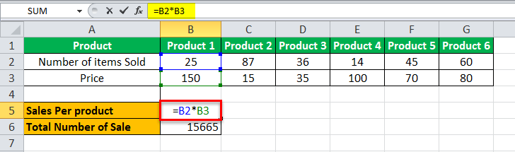
A restaurant’s sales data consists of each product’s price and the number of products sold.
The owner wants to calculate the total sales done by those products.

The owner multiplies the number of items sold for each product then sums them up as in the given-below equation,

Also, he gets the total sales as given below:

But this is a lengthy task. If the data were bigger, it would be much more tedious. So instead, Excel offers array of formulas for such tasks.

We will create our first array formula in cell B7.
The following are the steps to make the first array: –
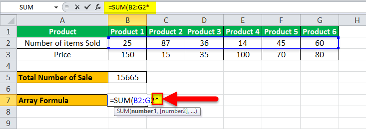
- In cell B7, type =SUM and press the “tab” button on the keyboard. It may open up the sum formula.

- Select the cell range from B2 to G2.

- Now, put an asterisk “*” sign after B2:G2 to multiply.

- Select the cell range from B3 to G3.

- Instead of pressing the “Enter” key, press “CTRL + SHIFT + ENTER.”

As a result, Excel may provide the total sales value by multiplying the number of products by the price in each column and summing them up. For example, in the highlighted section, we can see that Excel has created an array for cell range B2 to G2 and B3 to G3.

The above example explains how Excel array formulas return a single value for an array or set of data.


Example #2
With the same data, what if the owner wants to know the sales for each product separately, like sales of products 1 and 2?

He can either go a long way. In each cell, perform a function that will calculate the sales value.
The equation mentioned in cell B5 will be required to repeat for cells C4, D4, etc.
Again, it would be a tedious task if it were larger data.
In this example, we will learn how array formulas in Excel return multiple values for a set of arrays.

#1 – Select the cells where we want our subtotals, i.e., per product sales for each product. In this case, it is a cell range B8 to G8.

#2 – Type an equal to sign “=” a
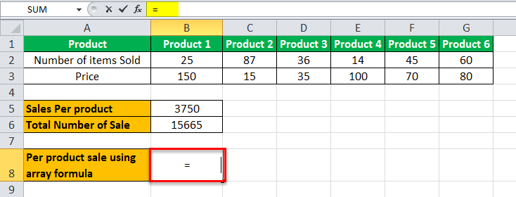
#3 –Select cell range B2 to G2.

#4 – Type an asterisk “*” sign after B2:G2.

#5 – Now, select cell range B3 to G3.

#6 – Do not press the “Enter” key for the array formula. Press “CTRL + SHIFT + ENTER” for array formula.

The above example explains how an array formula can return multiple values for an array in Excel.
Cells B6 to G6 are an array.
Example #3
For the same restaurant owner, he has the restaurant sales data for six months Jan, Feb, March, April, May, and June. He wants to know the average growth rate for sales.
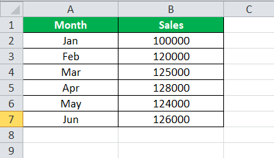
The owner can normally subtract the sales value of Feb month to Jan in cell C2 and then calculate the average.

Again, it would be a tiresome task if this were larger data. So let us do this with the array in Excel formulas.
#1 – In cell D8, type =average. Then, press the “tab” button.

#2 – To calculate growth, we will need to subtract the values of one month from the previous month to select the cell range from B3 to B7.

#3 – Put a subtract (-) sign after B3:B7,

#4 – Now, select cells from B2 to B6.
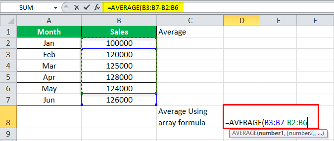
#5 – As for the array in Excel, do not press the “Enter” key. Press “CTRL + SHIFT + ENTER.”

Array formulas in Excel easily calculated the average growth for the sales without any hassle.
The owner now does not require calculating each month’s growth and performs the average function after that.
Things to Remember
- These are also known as CSE Formulas or Control Shift Enter ExcelCtrl-Shift Enter In Excel is a shortcut command that facilitates implementing the array formula in the excel function to execute an intricate computation of the given data. Altogether it transforms a particular data into an array format in excel with multiple data values for this purpose.read more Formulas.
- Do not make parenthesis for an array; Excel itself does that. It would return an error or incorrect value.
- Entering the parenthesis “{“manually, Excel will treat it as a text.
- Do not press the “Enter” key. Instead, press “CTRL + SHIFT + Enter” to use an array formula.
- We cannot change the cell of an array. So, to modify an array formula, either modify the formula from the function bar or delete the formula and redesign it in the desired format.
Recommended Articles
This article is a step-by-step guide to Array formulas in Excel. Here, we discuss how to use array in Excel using basic SUM and AVERAGE formulas and use it to solve array in Excel along with Excel examples and downloadable Excel templates. You may also look at these useful functions in Excel: –
- What is Name Range in Excel?
- Redim Array in Excel VBA
- Excel Formula Cheat Sheet
- VBA Array Function
Excel worksheet arrays and vectors
This material about arrays and vectors involves three concepts:
- Excel structures able to hold data, most commonly, the array of cells on a worksheet (by reference, name or constant)
- mathematical element wise array operations, and
- matrix based linear algebra array operations
An array can be described as a group of items that can be acted on either individually or collectively. An array’s orientation is classified by its dimension (such as column orientation, or row orientation, discussed further in section 1). In Excel the concept is best illustrated by example, see figure 1 (worksheet: WS arrays) where «a group of items» means a contiguous range, In particular, an array can be a:
- Scalar — a single cell
- Column array (column vector) — range
B2:B7shaded green - Row array (row vector) — range
B9:E9shaded blue - Multi dimensional array — range
B11:D14shaded grey
The expressions «scalar», «row vector» and «column vector» are common to the MatLab (matrix laboratory) application software.
1. Arrays — concepts
Dimension
The size of an array is described by the number of rows and number of columns. By convention the dimension is always rows first and columns second, in the spirit of R1C1 reference style, and the ordering of row and column arguments in functions such as INDEX and OFFSET.
Excel uses [mR x nR] during selection resizing operations (m and n are common to MatLab). MatLab uses m x n notation, with m being the number of rows (first dimension) and n being the number of columns (second dimension). Thus [2R x 3C] is a 2 row by 3 column array.
An array is contiguous, meaning rectangular / square, and a worksheet array can be referenced by the top left cell and bottom right cell with the range operator, see B11:DF14 in figure 1. Some functions return an array (eg. the TRANSPOSE and MMULT functions).
Dimensions (from figure 1):
- Scalar: dimension 1 x 1 (not shown in figure)
- Column vector: named
ColArr, dimension 6 x 1, number of elements 6 - Row vector: named
RowArr, dimension 1 x 4, number of elements 4 - MultiDimensional array: a two dimensional array named
MDArr, dimension 4 x 3, number of elements 12
In mathematics, the arrays in figure 1 can presented in the form:
$$text{ColArr}=begin{bmatrix} r1 \ r2 \ r3 \ r4 \ r5 \ r6 end{bmatrix},
qquad text{RowArr}=begin{bmatrix} c1 & c2 & c3 & c4 end{bmatrix}
qquad text{MDArr}=begin{bmatrix} r1c1 & r1c2 & r1c3 \ r2c1 & r2c2 & r2c3 \ r3c1 & r3c2 & r3c3 \ r4c1 & r4c2 & r4c3 end{bmatrix}$$
where [ ] represents the array.
Name Manager curly braces «{}»
In Excel there are two representations of arrays:
- the worksheet depiction in figure 1, and
- computer memory depictions such as the Value and Refers To field of the Name Manager (figure 2)
Value field
The three arrays from figure 1 are stored arrays link and are labeled ![]() in figure 2
in figure 2
- Excel arrays use opening «{» and closing «}» curly braces
- Arrays are constructed on a row by row basis
- Individual elements are separated by a comma «,»
- End of row is marked by a semi-colon «;» except for the last row
- These formats do not apply to a scalar
In Excel array notation:
- Name:
ColArr; Value:{"r1";"r2";"r3";"r4";"r5";"r6"} - Name:
RowArr; Value:{"c1","c2","c3","c4"} - Name:
MDArr; Value:{"r1c1","r1c2","r1c3";"r2c1","r2c2","r2c3";"r3c1","r3c2","r3c3";"r4c1","r4c2","r4c3"}
«Refers To» field
The array ArrConst, labeled ![]() in figure 2 is a named array constant. It has 2 x 2 dimension and is used in the Named Array Const worksheet in figure 3.
in figure 2 is a named array constant. It has 2 x 2 dimension and is used in the Named Array Const worksheet in figure 3.
In Excel array notation, the named array constant has:
- Name:
ArrConst; - Value:
{...}curly braces with a horizontal ellipses; - Refers To:
{"A",1;"XFD",1048576}
To enter the array, select a 2 x 2 range, type =ArrConst in the Formula Bar, then press Control + Shift + Enter to complete the formula.
A named array constant
- can contain numbers, text, logical values (TRUE and FALSE) and error values (like #N/A!)
- all text must be in double quotes «»
- cannot contain other arrays, formulas, or functions
- percentages must be decimal or text (0.10 or «10%»)
Function Arguments curly braces «{}»
Array values are displayed in the Function Arguments dialog box to the right of the argument name (figure 4). A maximum of 36 characters are shown.
Formula F2 F9 curly braces «{}»
You can check the values in an array (or reference) with the F2 F9 sequence. In figure 5, the cell F2 has the formula =COUNTA(ColArr). To check the values in the array
- switch to Edit mode by pressing F2
- select the reference
ColArrin the Formula Bar - press F9 to debug part of a formula. The result is displayed in the figure
- this technique is limited by the formula maximum of 8,192 characters (2 ^ 13)
2. Arrays — element wise operators
Operations on an array, as described in section 2, requires an array formula which has several distinct features compared to a conventional formula in Excel.
- An array formula is completed by pressing the CONTROL + SHIFT + ENTER key sequence often referred to by the abbreviation CSE formula
- There two distinct types of operations involving arrays
- Element by element, and
- Matrix (based on linear algebra)
- Only element by element is covered in this module
- (Generally) Each array must have the same magnitude and direction. In other words, the name dimension (excluding 1 x 1 scalar arrays)
- You cannot edit or delete part of an array. You must select the current array — use the Ctrl + / shortcut, or
Example — Excel Online #1
From the «element wise» worksheet in figure 6. The example uses two row vectors each of dimension (1 x 3). The range names of the arrays and values are: x = [1,2,3], and y = [4,5,6], and they appear in rows 4 and 5 of figure 6
WS1: the element wise worksheet demonstrates:
- Addition
- Subtraction
- Multiplication
- Division
- Scalar addition
- Scalar subtraction
- Scalar multiplication
- Scalar division
- Scalar exponentiation
- Scalar logical
WS2: The U x P >> Sales worksheet demonstrates a small data base of Unit number and Price data, the user is required to:
- Calculate Total Sales using normal cell formulae and the SUM function
- Calculate Total Sales using CSE formulae for sales then SUM
- Calculate Total Sales using CSE formulae in the final cell
- Repeat step 3 using the Excel SUMPRODUCT function
Each vector is 6 x 1.
WS3: The 100 records no IF filter worksheet uses the 100 records data base to demonstrate vector logical CSE formulas. Required:
- Sum product A, B and C for
Salesperson = "Wong" - Sum product A, B and C for
Salesperson = "Wong" AND Month = "September" - Sum product A for
Salesperson = "Wong" AND Product A >= 10 AND Product A <= 30
Each field column uses the label as vector name. For example, the Invoice No field has vector name Invoice_No
The CSE formulas are (in Ready mode):
{=SUM((Salesperson = "Wong") * Prod_C_qty)}{=SUM((Salesperson="Wong") * (Month="September") * Prod_C_qty)}{=SUM((Salesperson="Wong") * (Prod_A_qty >= 10) * (Prod_A_qty <= 30) * Prod_A_qty)}
WS4: The NPV as CSE worksheet uses using the VisiCalc handbook numbers, and the xlf Carrot Washer example.
The technique is a direct interpretation of the NPV equation —
$$begin{equation} NPV=sum_{t=0}^{n} frac{C_t}{(1+k)^t} end{equation}$$ where the initial cash flow at time zero and future cash flows at time (t) are denoted (C_t) over (n) periods. (k) is the periodic discount rate.
Using equation 1, the application is:
The VisiCalc example
$$ NPV=frac{-20,000}{(1+0.1)^{0}} + frac{3,000}{(1+0.1)^{1}} + frac{7,500}{(1+0.1)^{2}}+ frac{15,000}{(1+0.1)^{3}}+ frac{25,000}{(1+0.1)^{4}}+ frac{30,000}{(1+0.1)^{5}} = $35,898 $$
The carrot washer example
$$ NPV=frac{-80,000}{(1+0.05)^{0}} + frac{10,000}{(1+0.05)^{1}} + frac{20,000}{(1+0.05)^{2}}+ frac{15,000}{(1+0.05)^{3}}+ frac{50,000}{(1+0.05)^{4}}+ frac{20,000}{(1+0.05)^{5}} = $17,428 $$
The CSE formulas for the NPV estimates are:
- VisiCalc
=SUM(Cashflows / (1 + Disc) ^ {0;1;2;3;4;5})returns 35,898.32, where{0;1;2;3;4;5}is an array constant (column orientation 6 by 1) - carrot washer
=SUM(Cashflows2 / (1 + Disc2) ^ (ROW(1:6) - 1))returns 17,427.61
- Development platform: Excel 2016 (64 bit) Office 365 ProPlus on Windows 10
- Related material: Add a series of relative offset names to the Name Manager
- O’Connor I, (2015) Convert lower triangle table to full matrix. Includes discussion of array / matrix dimension and element indexing
- O’Connor I, (2017) Excel functions with array arguments. Includes array (CSE) and enter formulas
- O’Connor I, (2015) Vector to array constant. Includes VBA code for text based vector
- Revised: Saturday 25th of February 2023 — 10:12 AM, [Australian Eastern Time (AET)]
This post provides an in-depth look at the VBA array which is a very important part of the Excel VBA programming language. It covers everything you need to know about the VBA array.
We will start by seeing what exactly is the VBA Array is and why you need it.
Below you will see a quick reference guide to using the VBA Array. Refer to it anytime you need a quick reminder of the VBA Array syntax.
The rest of the post provides the most complete guide you will find on the VBA array.
Related Links for the VBA Array
Loops are used for reading through the VBA Array:
For Loop
For Each Loop
Other data structures in VBA:
VBA Collection – Good when you want to keep inserting items as it automatically resizes.
VBA ArrayList – This has more functionality than the Collection.
VBA Dictionary – Allows storing a KeyValue pair. Very useful in many applications.
The Microsoft guide for VBA Arrays can be found here.
A Quick Guide to the VBA Array
| Task | Static Array | Dynamic Array |
|---|---|---|
| Declare | Dim arr(0 To 5) As Long | Dim arr() As Long Dim arr As Variant |
| Set Size | See Declare above | ReDim arr(0 To 5)As Variant |
| Get Size(number of items) | See ArraySize function below. | See ArraySize function below. |
| Increase size (keep existing data) | Dynamic Only | ReDim Preserve arr(0 To 6) |
| Set values | arr(1) = 22 | arr(1) = 22 |
| Receive values | total = arr(1) | total = arr(1) |
| First position | LBound(arr) | LBound(arr) |
| Last position | Ubound(arr) | Ubound(arr) |
| Read all items(1D) | For i = LBound(arr) To UBound(arr) Next i Or For i = LBound(arr,1) To UBound(arr,1) Next i |
For i = LBound(arr) To UBound(arr) Next i Or For i = LBound(arr,1) To UBound(arr,1) Next i |
| Read all items(2D) | For i = LBound(arr,1) To UBound(arr,1) For j = LBound(arr,2) To UBound(arr,2) Next j Next i |
For i = LBound(arr,1) To UBound(arr,1) For j = LBound(arr,2) To UBound(arr,2) Next j Next i |
| Read all items | Dim item As Variant For Each item In arr Next item |
Dim item As Variant For Each item In arr Next item |
| Pass to Sub | Sub MySub(ByRef arr() As String) | Sub MySub(ByRef arr() As String) |
| Return from Function | Function GetArray() As Long() Dim arr(0 To 5) As Long GetArray = arr End Function |
Function GetArray() As Long() Dim arr() As Long GetArray = arr End Function |
| Receive from Function | Dynamic only | Dim arr() As Long Arr = GetArray() |
| Erase array | Erase arr *Resets all values to default |
Erase arr *Deletes array |
| String to array | Dynamic only | Dim arr As Variant arr = Split(«James:Earl:Jones»,»:») |
| Array to string | Dim sName As String sName = Join(arr, «:») |
Dim sName As String sName = Join(arr, «:») |
| Fill with values | Dynamic only | Dim arr As Variant arr = Array(«John», «Hazel», «Fred») |
| Range to Array | Dynamic only | Dim arr As Variant arr = Range(«A1:D2») |
| Array to Range | Same as dynamic | Dim arr As Variant Range(«A5:D6») = arr |
Download the Source Code and Data
Please click on the button below to get the fully documented source code for this article.
What is the VBA Array and Why do You Need It?
A VBA array is a type of variable. It is used to store lists of data of the same type. An example would be storing a list of countries or a list of weekly totals.
In VBA a normal variable can store only one value at a time.
In the following example we use a variable to store the marks of a student:
' Can only store 1 value at a time
Dim Student1 As Long
Student1 = 55
If we wish to store the marks of another student then we need to create a second variable.
In the following example, we have the marks of five students:

Student Marks
We are going to read these marks and write them to the Immediate Window.
Note: The function Debug.Print writes values to the Immediate Window. To view this window select View->Immediate Window from the menu( Shortcut is Ctrl + G)


As you can see in the following example we are writing the same code five times – once for each student:
' https://excelmacromastery.com/
Public Sub StudentMarks()

    ' Get the worksheet called "Marks"
    Dim sh As Worksheet
    Set sh = ThisWorkbook.Worksheets("Marks")

    ' Declare variable for each student
    Dim Student1 As Long
    Dim Student2 As Long
    Dim Student3 As Long
    Dim Student4 As Long
    Dim Student5 As Long

    ' Read student marks from cell
    Student1 = sh.Range("C" & 3).Value
    Student2 = sh.Range("C" & 4).Value
    Student3 = sh.Range("C" & 5).Value
    Student4 = sh.Range("C" & 6).Value
    Student5 = sh.Range("C" & 7).Value

    ' Print student marks
    Debug.Print "Students Marks"
    Debug.Print Student1
    Debug.Print Student2
    Debug.Print Student3
    Debug.Print Student4
    Debug.Print Student5

End Sub
The following is the output from the example:

Output
The problem with using one variable per student is that you need to add code for each student. Therefore if you had a thousand students in the above example you would need three thousand lines of code!
Luckily we have arrays to make our life easier. Arrays allow us to store a list of data items in one structure.
The following code shows the above student example using an array:
' ExcelMacroMastery.com
' https://excelmacromastery.com/excel-vba-array/
' Author: Paul Kelly
' Description: Reads marks to an Array and write
' the array to the Immediate Window(Ctrl + G)
' TO RUN: Click in the sub and press F5
Public Sub StudentMarksArr()

    ' Get the worksheet called "Marks"
    Dim sh As Worksheet
    Set sh = ThisWorkbook.Worksheets("Marks")

    ' Declare an array to hold marks for 5 students
    Dim Students(1 To 5) As Long

    ' Read student marks from cells C3:C7 into array
    ' Offset counts rows from cell C2.
    ' e.g. i=1 is C2 plus 1 row which is C3
    '      i=2 is C2 plus 2 rows which is C4
    Dim i As Long
    For i = 1 To 5
        Students(i) = sh.Range("C2").Offset(i).Value
    Next i

    ' Print student marks from the array to the Immediate Window
    Debug.Print "Students Marks"
    For i = LBound(Students) To UBound(Students)
        Debug.Print Students(i)
    Next i

End Sub
The advantage of this code is that it will work for any number of students. If we have to change this code to deal with 1000 students we only need to change the (1 To 5) to (1 To 1000) in the declaration. In the prior example we would need to add approximately five thousand lines of code.
Let’s have a quick comparison of variables and arrays. First we compare the declaration:
        ' Variable
        Dim Student As Long
        Dim Country As String

        ' Array
        Dim Students(1 To 3) As Long
        Dim Countries(1 To 3) As String
Next we compare assigning a value:
        ' assign value to variable
        Student1 = .Cells(1, 1)

        ' assign value to first item in array
        Students(1) = .Cells(1, 1)
Finally we look at writing the values:
        ' Print variable value
        Debug.Print Student1

        ' Print value of first student in array
        Debug.Print Students(1)
As you can see, using variables and arrays is quite similar.
The fact that arrays use an index(also called a subscript) to access each item is important. It means we can easily access all the items in an array using a For Loop.
Now that you have some background on why arrays are useful let’s go through them step by step.
Two Types of VBA Arrays
There are two types of VBA arrays:
- Static – an array of fixed length.
- Dynamic(not to be confused with the Excel Dynamic Array) – an array where the length is set at run time.
The difference between these types is mostly in how they are created. Accessing values in both array types is exactly the same. In the following sections we will cover both of these types.
VBA Array Initialization
A static array is initialized as follows:
' https://excelmacromastery.com/
Public Sub DecArrayStatic()

    ' Create array with locations 0,1,2,3
    Dim arrMarks1(0 To 3) As Long

    ' Defaults as 0 to 3 i.e. locations 0,1,2,3
    Dim arrMarks2(3) As Long

    ' Create array with locations 1,2,3,4,5
    Dim arrMarks3(1 To 5) As Long

    ' Create array with locations 2,3,4 ' This is rarely used
    Dim arrMarks4(2 To 4) As Long

End Sub
![]()
An Array of 0 to 3
As you can see the length is specified when you declare a static array. The problem with this is that you can never be sure in advance the length you need. Each time you run the Macro you may have different length requirements.
If you do not use all the array locations then the resources are being wasted. So if you need more locations you can use ReDim but this is essentially creating a new static array.
The dynamic array does not have such problems. You do not specify the length when you declare it. Therefore you can then grow and shrink as required:
' https://excelmacromastery.com/
Public Sub DecArrayDynamic()

    ' Declare  dynamic array
    Dim arrMarks() As Long

    ' Set the length of the array when you are ready
    ReDim arrMarks(0 To 5)

End Sub
The dynamic array is not allocated until you use the ReDim statement. The advantage is you can wait until you know the number of items before setting the array length. With a static array you have to state the length upfront.
To give an example. Imagine you were reading worksheets of student marks. With a dynamic array you can count the students on the worksheet and set an array to that length. With a static array you must set the length to the largest possible number of students.
Assigning Values to VBA Array
To assign values to an array you use the number of the location. You assign the value for both array types the same way:
' https://excelmacromastery.com/
Public Sub AssignValue()

    ' Declare  array with locations 0,1,2,3
    Dim arrMarks(0 To 3) As Long

    ' Set the value of position 0
    arrMarks(0) = 5

    ' Set the value of position 3
    arrMarks(3) = 46

    ' This is an error as there is no location 4
    arrMarks(4) = 99

End Sub
![]()
The array with values assigned
The number of the location is called the subscript or index. The last line in the example will give a “Subscript out of Range” error as there is no location 4 in the array example.
VBA Array Length
There is no native function for getting the number of items in an array. I created the ArrayLength function below to return the number of items in any array no matter how many dimensions:
' https://excelmacromastery.com/
Function ArrayLength(arr As Variant) As Long

    On Error Goto eh

    ' Loop is used for multidimensional arrays. The Loop will terminate when a
    ' "Subscript out of Range" error occurs i.e. there are no more dimensions.
    Dim i As Long, length As Long
    length = 1

    ' Loop until no more dimensions
    Do While True
        i = i + 1
        ' If the array has no items then this line will throw an error
        Length = Length * (UBound(arr, i) - LBound(arr, i) + 1)
        ' Set ArrayLength here to avoid returing 1 for an empty array
        ArrayLength = Length
    Loop

Done:
    Exit Function
eh:
    If Err.Number = 13 Then ' Type Mismatch Error
        Err.Raise vbObjectError, "ArrayLength" _
            , "The argument passed to the ArrayLength function is not an array."
    End If
End Function
You can use it like this:
' Name: TEST_ArrayLength
' Author: Paul Kelly, ExcelMacroMastery.com
' Description: Tests the ArrayLength functions and writes
'              the results to the Immediate Window(Ctrl + G)
Sub TEST_ArrayLength()

    ' 0 items
    Dim arr1() As Long
    Debug.Print ArrayLength(arr1)

    ' 10 items
    Dim arr2(0 To 9) As Long
    Debug.Print ArrayLength(arr2)

    ' 18 items
    Dim arr3(0 To 5, 1 To 3) As Long
    Debug.Print ArrayLength(arr3)

    ' Option base 0: 144 items
    ' Option base 1: 50 items
    Dim arr4(1, 5, 5, 0 To 1) As Long
    Debug.Print ArrayLength(arr4)

End Sub
Using the Array and Split function
You can use the Array function to populate an array with a list of items. You must declare the array as a type Variant. The following code shows you how to use this function.
    Dim arr1 As Variant
    arr1 = Array("Orange", "Peach","Pear")

    Dim arr2 As Variant
    arr2 = Array(5, 6, 7, 8, 12)

Contents of arr1 after using the Array function
The array created by the Array Function will start at index zero unless you use Option Base 1 at the top of your module. Then it will start at index one. In programming, it is generally considered poor practice to have your actual data in the code. However, sometimes it is useful when you need to test some code quickly.
The Split function is used to split a string into an array based on a delimiter. A delimiter is a character such as a comma or space that separates the items.
The following code will split the string into an array of four elements:
    Dim s As String
    s = "Red,Yellow,Green,Blue"

    Dim arr() As String
    arr = Split(s, ",")
![]()
The array after using Split
The Split function is normally used when you read from a comma-separated file or another source that provides a list of items separated by the same character.
Using Loops With the VBA Array
Using a For Loop allows quick access to all items in an array. This is where the power of using arrays becomes apparent. We can read arrays with ten values or ten thousand values using the same few lines of code. There are two functions in VBA called LBound and UBound. These functions return the smallest and largest subscript in an array. In an array arrMarks(0 to 3) the LBound will return 0 and UBound will return 3.
The following example assigns random numbers to an array using a loop. It then prints out these numbers using a second loop.
' https://excelmacromastery.com/
Public Sub ArrayLoops()

    ' Declare  array
    Dim arrMarks(0 To 5) As Long

    ' Fill the array with random numbers
    Dim i As Long
    For i = LBound(arrMarks) To UBound(arrMarks)
        arrMarks(i) = 5 * Rnd
    Next i

    ' Print out the values in the array
    Debug.Print "Location", "Value"
    For i = LBound(arrMarks) To UBound(arrMarks)
        Debug.Print i, arrMarks(i)
    Next i

End Sub
The functions LBound and UBound are very useful. Using them means our loops will work correctly with any array length. The real benefit is that if the length of the array changes we do not have to change the code for printing the values. A loop will work for an array of any length as long as you use these functions.
Using the For Each Loop with the VBA Array
You can use the For Each loop with arrays. The important thing to keep in mind is that it is Read-Only. This means that you cannot change the value in the array.
In the following code the value of mark changes but it does not change the value in the array.
    For Each mark In arrMarks
        ' Will not change the array value
        mark = 5 * Rnd
    Next mark
The For Each is loop is fine to use for reading an array. It is neater to write especially for a Two-Dimensional array as we will see.
    Dim mark As Variant
    For Each mark In arrMarks
        Debug.Print mark
    Next mark
Using Erase with the VBA Array
The Erase function can be used on arrays but performs differently depending on the array type.
For a static Array the Erase function resets all the values to the default. If the array is made up of long integers(i.e type Long) then all the values are set to zero. If the array is of strings then all the strings are set to “” and so on.
For a Dynamic Array the Erase function DeAllocates memory. That is, it deletes the array. If you want to use it again you must use ReDim to Allocate memory.
Let’s have a look an example for the static array. This example is the same as the ArrayLoops example in the last section with one difference – we use Erase after setting the values. When the value are printed out they will all be zero:
' https://excelmacromastery.com/
Public Sub EraseStatic()

    ' Declare  array
    Dim arrMarks(0 To 3) As Long

    ' Fill the array with random numbers
    Dim i As Long
    For i = LBound(arrMarks) To UBound(arrMarks)
        arrMarks(i) = 5 * Rnd
    Next i

    ' ALL VALUES SET TO ZERO
    Erase arrMarks

    ' Print out the values - there are all now zero
    Debug.Print "Location", "Value"
    For i = LBound(arrMarks) To UBound(arrMarks)
        Debug.Print i, arrMarks(i)
    Next i

End Sub
We will now try the same example with a dynamic. After we use Erase all the locations in the array have been deleted. We need to use ReDim if we wish to use the array again.
If we try to access members of this array we will get a “Subscript out of Range” error:
' https://excelmacromastery.com/
Public Sub EraseDynamic()

    ' Declare  array
    Dim arrMarks() As Long
    ReDim arrMarks(0 To 3)

    ' Fill the array with random numbers
    Dim i As Long
    For i = LBound(arrMarks) To UBound(arrMarks)
        arrMarks(i) = 5 * Rnd
    Next i

    ' arrMarks is now deallocated. No locations exist.
    Erase arrMarks

End Sub
Increasing the length of the VBA Array
If we use ReDim on an existing array, then the array and its contents will be deleted.
In the following example, the second ReDim statement will create a completely new array. The original array and its contents will be deleted.
' https://excelmacromastery.com/
Sub UsingRedim()

    Dim arr() As String

    ' Set array to be slots 0 to 2
    ReDim arr(0 To 2)
    arr(0) = "Apple"

    ' Array with apple is now deleted
    ReDim arr(0 To 3)

End Sub
If we want to extend the length of an array without losing the contents, we can use the Preserve keyword.
When we use Redim Preserve the new array must start at the same starting dimension e.g.
We cannot Preserve from (0 to 2) to (1 to 3) or to (2 to 10) as they are different starting dimensions.
In the following code we create an array using ReDim and then fill the array with types of fruit.
We then use Preserve to extend the length of the array so we don’t lose the original contents:
' https://excelmacromastery.com/
Sub UsingRedimPreserve()

    Dim arr() As String

    ' Set array to be slots 0 to 1
    ReDim arr(0 To 2)
    arr(0) = "Apple"
    arr(1) = "Orange"
    arr(2) = "Pear"

    ' Reset the length and keep original contents
    ReDim Preserve arr(0 To 5)

End Sub
You can see from the screenshots below, that the original contents of the array have been “Preserved”.

Before ReDim Preserve

After ReDim Preserve
Word of Caution: In most cases, you shouldn’t need to resize an array like we have done in this section. If you are resizing an array multiple times then you may want to consider using a Collection.
Using Preserve with Two-Dimensional Arrays
Preserve only works with the upper bound of an array.
For example, if you have a two-dimensional array you can only preserve the second dimension as this example shows:
' https://excelmacromastery.com/
Sub Preserve2D()

    Dim arr() As Long

    ' Set the starting length
    ReDim arr(1 To 2, 1 To 5)

    ' Change the length of the upper dimension
    ReDim Preserve arr(1 To 2, 1 To 10)

End Sub
If we try to use Preserve on a lower bound we will get the “Subscript out of range” error.
In the following code we use Preserve on the first dimension. Running this code will give the “Subscript out of range” error:
' https://excelmacromastery.com/
Sub Preserve2DError()

    Dim arr() As Long

    ' Set the starting length
    ReDim arr(1 To 2, 1 To 5)

    ' "Subscript out of Range" error
    ReDim Preserve arr(1 To 5, 1 To 5)

End Sub
When we read from a range to an array, it automatically creates a two-dimensional array, even if we have only one column.
The same Preserve rules apply. We can only use Preserve on the upper bound as this example shows:
' https://excelmacromastery.com/
Sub Preserve2DRange()

    Dim arr As Variant

    ' Assign a range to an array
    arr = Sheet1.Range("A1:A5").Value

    ' Preserve will work on the upper bound only
    ReDim Preserve arr(1 To 5, 1 To 7)

End Sub
Sorting the VBA Array
There is no function in VBA for sorting an array. We can sort the worksheet cells but this could be slow if there is a lot of data.
The QuickSort function below can be used to sort an array.
' https://excelmacromastery.com/
Sub QuickSort(arr As Variant, first As Long, last As Long)

  Dim vCentreVal As Variant, vTemp As Variant

  Dim lTempLow As Long
  Dim lTempHi As Long
  lTempLow = first
  lTempHi = last

  vCentreVal = arr((first + last)  2)
  Do While lTempLow <= lTempHi

    Do While arr(lTempLow) < vCentreVal And lTempLow < last
      lTempLow = lTempLow + 1
    Loop

    Do While vCentreVal < arr(lTempHi) And lTempHi > first
      lTempHi = lTempHi - 1
    Loop

    If lTempLow <= lTempHi Then

        ' Swap values
        vTemp = arr(lTempLow)

        arr(lTempLow) = arr(lTempHi)
        arr(lTempHi) = vTemp

        ' Move to next positions
        lTempLow = lTempLow + 1
        lTempHi = lTempHi - 1

    End If

  Loop

  If first < lTempHi Then QuickSort arr, first, lTempHi
  If lTempLow < last Then QuickSort arr, lTempLow, last

End Sub
You can use this function like this:
' https://excelmacromastery.com/
Sub TestSort()

    ' Create temp array
    Dim arr() As Variant
    arr = Array("Banana", "Melon", "Peach", "Plum", "Apple")

    ' Sort array
    QuickSort arr, LBound(arr), UBound(arr)

    ' Print arr to Immediate Window(Ctrl + G)
    Dim i As Long
    For i = LBound(arr) To UBound(arr)
        Debug.Print arr(i)
    Next i

End Sub
Passing the VBA Array to a Sub
Sometimes you will need to pass an array to a procedure. You declare the parameter using parenthesis similar to how you declare a dynamic array.
Passing to the procedure using ByRef means you are passing a reference of the array. So if you change the array in the procedure it will be changed when you return.
Note: When you use an array as a parameter it cannot use ByVal, it must use ByRef. You can pass the array using ByVal making the parameter a variant.
' https://excelmacromastery.com/
' Passes array to a Function
Public Sub PassToProc()
    Dim arr(0 To 5) As String
    ' Pass the array to function
    UseArray arr
End Sub

Public Function UseArray(ByRef arr() As String)
    ' Use array
    Debug.Print UBound(arr)
End Function
Returning the VBA Array from a Function
It is important to keep the following in mind. If you want to change an existing array in a procedure then you should pass it as a parameter using ByRef(see last section). You do not need to return the array from the procedure.
The main reason for returning an array is when you use the procedure to create a new one. In this case you assign the return array to an array in the caller. This array cannot be already allocated. In other words you must use a dynamic array that has not been allocated.
The following examples show this
' https://excelmacromastery.com/
Public Sub TestArray()

    ' Declare dynamic array - not allocated
    Dim arr() As String
    ' Return new array
    arr = GetArray

End Sub

Public Function GetArray() As String()

    ' Create and allocate new array
    Dim arr(0 To 5) As String
    ' Return array
    GetArray = arr

End Function
Using a Two-Dimensional VBA Array
The arrays we have been looking at so far have been one-dimensional arrays. This means the arrays are one list of items.
A two-dimensional array is essentially a list of lists. If you think of a single spreadsheet row as a single dimension then more than one column is two dimensional. In fact a spreadsheet is the equivalent of a two-dimensional array. It has two dimensions – rows and columns.
One small thing to note is that Excel treats a one-dimensional array as a row if you write it to a spreadsheet. In other words, the array arr(1 to 5) is equivalent to arr(1 to 1, 1 to 5) when writing values to the spreadsheet.
The following image shows two groups of data. The first is a one-dimensional layout and the second is two dimensional.

To access an item in the first set of data(1 dimensional) all you need to do is give the row e.g. 1,2, 3 or 4.
For the second set of data (two-dimensional), you need to give the row AND the column. So you can think of 1 dimensional being multiple columns and one row and two-dimensional as being multiple rows and multiple columns.
Note: It is possible to have more than two dimensions in an array. It is rarely required. If you are solving a problem using a 3+ dimensional array then there probably is a better way to do it.
You declare a two-dimensional array as follows:
Dim ArrayMarks(0 To 2,0 To 3) As Long
The following example creates a random value for each item in the array and the prints the values to the Immediate Window:
' https://excelmacromastery.com/
Public Sub TwoDimArray()

    ' Declare a two dimensional array
    Dim arrMarks(0 To 3, 0 To 2) As String

    ' Fill the array with text made up of i and j values
    Dim i As Long, j As Long
    For i = LBound(arrMarks) To UBound(arrMarks)
        For j = LBound(arrMarks, 2) To UBound(arrMarks, 2)
            arrMarks(i, j) = CStr(i) & ":" & CStr(j)
        Next j
    Next i

    ' Print the values in the array to the Immediate Window
    Debug.Print "i", "j", "Value"
    For i = LBound(arrMarks) To UBound(arrMarks)
        For j = LBound(arrMarks, 2) To UBound(arrMarks, 2)
            Debug.Print i, j, arrMarks(i, j)
        Next j
    Next i

End Sub
You can see that we use a second For loop inside the first loop to access all the items.
The output of the example looks like this:

How this Macro works is as follows:
- Enters the i loop
- i is set to 0
- Entersj loop
- j is set to 0
- j is set to 1
- j is set to 2
- Exit j loop
- i is set to 1
- j is set to 0
- j is set to 1
- j is set to 2
- And so on until i=3 and j=2
You may notice that LBound and UBound have a second argument with the value 2. This specifies that it is the upper or lower bound of the second dimension. That is the start and end location for j. The default value 1 which is why we do not need to specify it for the i loop.
Using the For Each Loop
Using a For Each is neater to use when reading from an array.
Let’s take the code from above that writes out the two-dimensional array
    ' Using For loop needs two loops
    Debug.Print "i", "j", "Value"
    For i = LBound(arrMarks) To UBound(arrMarks)
        For j = LBound(arrMarks, 2) To UBound(arrMarks, 2)
            Debug.Print i, j, arrMarks(i, j)
        Next j
    Next i
Now let’s rewrite it using a For each loop. You can see we only need one loop and so it is much easier to write:
    ' Using For Each requires only one loop
    Debug.Print "Value"
    Dim mark As Variant
    For Each mark In arrMarks
        Debug.Print mark
    Next mark
Using the For Each loop gives us the array in one order only – from LBound to UBound. Most of the time this is all you need.
Reading from a Range to the VBA Array
If you have read my previous post on Cells and Ranges then you will know that VBA has an extremely efficient way of reading from a Range of Cells to an Array and vice versa
' https://excelmacromastery.com/
Public Sub ReadToArray()

    ' Declare dynamic array
    Dim StudentMarks As Variant

    ' Read values into array from first row
    StudentMarks = Range("A1:Z1").Value

    ' Write the values back to the third row
    Range("A3:Z3").Value = StudentMarks

End Sub
The dynamic array created in this example will be a two dimensional array. As you can see we can read from an entire range of cells to an array in just one line.
The next example will read the sample student data below from C3:E6 of Sheet1 and print them to the Immediate Window:
' https://excelmacromastery.com/
Public Sub ReadAndDisplay()

    ' Get Range
    Dim rg As Range
    Set rg = ThisWorkbook.Worksheets("Sheet1").Range("C3:E6")

    ' Create dynamic array
    Dim StudentMarks As Variant

    ' Read values into array from sheet1
    StudentMarks = rg.Value

    ' Print the array values
    Debug.Print "i", "j", "Value"
    Dim i As Long, j As Long
    For i = LBound(StudentMarks) To UBound(StudentMarks)
        For j = LBound(StudentMarks, 2) To UBound(StudentMarks, 2)
            Debug.Print i, j, StudentMarks(i, j)
        Next j
    Next i

End Sub

Sample Student data

Output from sample data
As you can see the first dimension(accessed using i) of the array is a row and the second is a column. To demonstrate this take a look at the value 44 in E4 of the sample data. This value is in row 2 column 3 of our data. You can see that 44 is stored in the array at StudentMarks(2,3).
You can see more about using arrays with ranges in this YouTube video
How To Make Your Macros Run at Super Speed
If your macros are running very slow then you may find this section very helpful. Especially if you are dealing with large amounts of data. The following is a very well-kept secret in VBA
Updating values in arrays is exponentially faster than updating values in cells.
In the last section, you saw how we can easily read from a group of cells to an array and vice versa. If we are updating a lot of values then we can do the following:
1. Copy the data from the cells to an array.
2. Change the data in the array.
3. Copy the updated data from the array back to the cells.
For example, the following code would be much faster than the code below it:
' https://excelmacromastery.com/
Public Sub ReadToArray()

    ' Read values into array from first row
    Dim StudentMarks  As Variant
    StudentMarks = Range("A1:Z20000").Value

    Dim i As Long
    For i = LBound(StudentMarks) To UBound(StudentMarks)
        ' Update marks here
        StudentMarks(i, 1) = StudentMarks(i, 1) * 2
        '...
    Next i

    ' Write the new values back to the worksheet
    Range("A1:Z20000").Value = StudentMarks

End Sub
' https://excelmacromastery.com/
Sub UsingCellsToUpdate()

    Dim c As Variant
    For Each c In Range("A1:Z20000")
        c.Value = ' Update values here
    Next c

End Sub
Assigning from one set of cells to another is also much faster than using Copy and Paste:
' Assigning - this is faster
Range("A1:A10").Value = Range("B1:B10").Value

' Copy Paste - this is slower
Range("B1:B1").Copy Destination:=Range("A1:A10")
The following comments are from two readers who used arrays to speed up their macros
“A couple of my projects have gone from almost impossible and long to run into almost too easy and a reduction in time to run from 10:1.” – Dane
“One report I did took nearly 3 hours to run when accessing the cells directly — 5 minutes with arrays” – Jim
You can see more about the speed of Arrays compared to other methods in this YouTube video.
To see a comparison between Find, Match and Arrays it is worth checking out this post by Charles Williams.
Conclusion
The following is a summary of the main points of this post
- Arrays are an efficient way of storing a list of items of the same type.
- You can access an array item directly using the number of the location which is known as the subscript or index.
- The common error “Subscript out of Range” is caused by accessing a location that does not exist.
- There are two types of arrays: Static and Dynamic.
- Static is used when the length of the array is always the same.
- Dynamic arrays allow you to determine the length of an array at run time.
- LBound and UBound provide a safe way of find the smallest and largest subscripts of the array.
- The basic array is one dimensional. You can also have multidimensional arrays.
- You can only pass an array to a procedure using ByRef. You do this like this: ByRef arr() as long.
- You can return an array from a function but the array, it is assigned to, must not be currently allocated.
- A worksheet with its rows and columns is essentially a two-dimensional array.
- You can read directly from a worksheet range into a two-dimensional array in just one line of code.
- You can also write from a two-dimensional array to a range in just one line of code.
What’s Next?
Free VBA Tutorial If you are new to VBA or you want to sharpen your existing VBA skills then why not try The Ultimate VBA Tutorial.
Related Training: Get full access to the Excel VBA training webinars.
(NOTE: Planning to build or manage a VBA Application? Learn how to build 10 Excel VBA applications from scratch.)
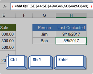
In Excel, an Array Formula allows you to do powerful calculations on one or more value sets. The result may fit in a single cell or it may be an array. An array is just a list or range of values, but an Array Formula is a special type of formula that must be entered by pressing Ctrl+Shift+Enter. The formula bar will show the formula surrounded by curly brackets {=…}.
Array formulas are frequently used for data analysis, conditional sums and lookups, linear algebra, matrix math and manipulation, and much more. A new Excel user might come across array formulas in other people’s spreadsheets, but creating array formulas is typically an intermediate-to-advanced topic.
Download the Example File (ArrayFormulas.xlsx)
Topics and Examples in This Article:
- Entering an Array Formula
- Using Array Constants
- A Simple Array Formula Example
- Entering a Multi-Cell Array Formula
- Nested IF Array Formulas
- COUNTIF Alternative: SUM-Boolean Array Formulas
- Multi-Criteria Boolean Array Formulas
- Sequential Number Arrays (1,2,3,…)
- Formulas for Matrices: MUNIT, MMULT, TRANSPOSE, etc.
- Other Array Formula Examples
Watch the Intro Video
Entering and Identifying an Array Formula
- When using an Array Formula, you press Ctrl+Shift+Enter instead of just Enter after entering or editing the formula. This is why array formulas are often called CSE formulas.
- An Array Formula will show curly brackets or braces around the formula in the Formula Bar like this: {=SUM(A1:A5*B1:B5)}
- Array Constants (arrays «hard-coded» into formulas) are enclosed in braces { } and use commas to separate columns, and semi-colons to separate rows, like this 2×3 array: {1, 1, 1; 2, 2, 2}
- If an Array Formula returns more than one value (a multi-cell array formula), first select a range of cells equal to size of the returned array, then enter your formula.
- To select all the cells within a multi-cell array: Press F5 > Special > Current Array.
! Every time you edit an Array Formula, you must remember to press Ctrl+Shift+Enter afterward. If you forget to, the formula may return an error without you realizing it.
NOTE Google Sheets uses the ARRAYFORMULA function instead of showing the formula surrounded by braces. It is not necessary to press Ctrl+Shift+Enter in Google Sheets, but if you do, ARRAYFORMULA( is added to the beginning of the formula.
Using Array Constants in Formulas
Many functions allow you use array constants like {1,2,6,12} as arguments within formulas. An example that I often use in my yearly calendar templates returns the weekday abbreviation for a given date. The nice thing about this formula is that you can choose whether to display a single character or two characters.
=INDEX({"Su";"M";"Tu";"W";"Th";"F";"Sa"},WEEKDAY(theDate,1))
This formula is not technically an Array Formula because you don’t enter it using Ctrl+Shift+Enter. Using a hard-coded array within a formula does not necessarily require using Ctrl+Shift+Enter.
TIP If you are going to use the array constant in multiple formulas, you may want to first create a Named Constant. Go to Formulas > Name Manager > New Name, enter a descriptive name like payment_frequency and enter ={1,2,6,12} into the Refers To field. You can use the name within your formulas. If you ever want to change the values within that array constant, you only need to change it one place (within the Name Manager).
A Simple Array Formula Example
To start out, I will show how an array formula works using a very basic example. Let’s say that I have a list of tasks, the number of days each of those tasks will take, and a column for the percent complete. I want to know the total number of days that have been completed.
Without an array formula, you would create another column called «Completed» and multiply the number of days by the % complete, and copy the formula down. Then I would use SUM to total the number of days completed, like the image below:
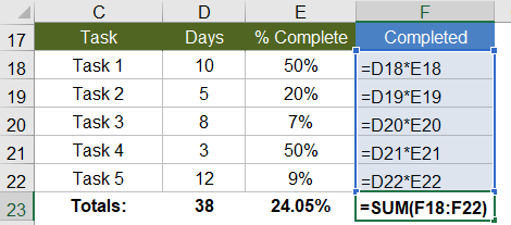
With an array formula, you can do essentially the same thing without having to create the extra column. Within a single cell, you can calculate the total days completed as =SUM(D18:D22*E18:E22), remembering to press Ctrl+Shift+Enter because it is an array formula.
{ =SUM(D18:D22*E18:E22) }

Evaluation Steps
Step 1: =SUM( {10;5;8;3;12} * {0.5;0.2;0.07;0.5;0.09} )
Step 2: =SUM( {10*0.5;5*0.2;8*0.7;3*0.5;12*0.09} )
Step 3: =SUM( {5;1;0.56;1.5;1.08} )
Step 4: =9.14
In this and other examples, I’ve shown the evaluation steps below the formula so that you can see how the formula works. You don’t actually type the curly brackets { }, but in this article I will surround all array formulas with brackets to indicate that they are entered as CSE formulas.
In the evaluation steps shown in the above example, you’ll see that Excel is multiplying each element of the first array by the corresponding element in the second array, and then SUM adds the results.
NOTE It turns out that this particular example can be used to show how the SUMPRODUCT function works, but the SUMPRODUCT function deserves its own article.
To take this example just a bit further, if all we wanted to know was the Total Percent Complete for the entire project, we can divide the total days completed (9.14) by the total days (38) all within a single array formula, and we don’t need column F at all (as shown in the image below).
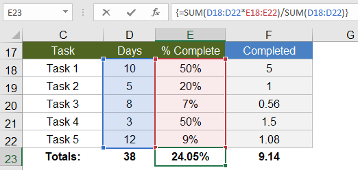
This example is an example of a single-cell array formula, meaning that the formula is entered into a single cell.
Entering a Multi-Cell Array Formula
Whenever your array formula returns more than one value, if you want to display more than just the first value, you need to select the range of cells that will contain the resulting array before entering your formula. Doing this will result in a multi-cell array formula, meaning that the result of the formula is a multi-cell array.
Using the same example as above, we could use an array formula in the Completed column to calculate Days * Percent Complete. First, select cells F18:F22, then press = and enter the formula, followed by Ctrl+Shift+Enter (CSE). The image below is what it will look like just before you press CSE.
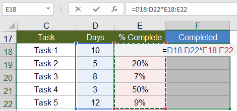
You can edit a multi-cell array formula by selecting any of the cells in the array and then updating the formula and pressing Ctrl+Shift+Enter when you are done. However, you can’t use this technique to modify the size of the array.
«You can’t change part of an array» — This is the warning or error you will get if you try to insert rows or columns or change individual cells within a multi-cell array.
Using multi-cell array formulas can make it more difficult to customize a spreadsheet because to change the size of the array requires that you (1) delete the formula (after selecting all the cells of the array), (2) select the new range of cells, and (3) re-enter the array formula. TIP: Make sure to copy your original formula before deleting it. Then, when you re-enter the formula, you can paste it and modify the ranges.
Nested IF Array Formulas
A nested IF array formula can be very powerful and is probably one of the more common uses for array formulas in Excel. Although Excel provides the SUMIF and COUNTIF and AVERAGEIF functions, they don’t allow as much freedom as a nested IF array formula.
MAX-IF Array Formula
Older versions of Excel do not have the MAXIFS or MINIFS functions, so let’s create our own MAX-IF formula. When we use hyphens to name a formula, it usually means that we’re nesting the functions (IF within MAX in this case).
Let’s say that I have the following contact and sales log and I want a formula that will tell me when I last contacted Bob (cell H51).
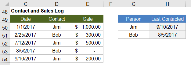
Using MAX on the date range will give me that latest date (9/10/2017), but I only want to include the rows where the contact is Bob. So, I’ll use the MAX-IF array formula:
{ =MAX(IF(contact_range="Bob",date_range)) }

Evaluation Steps
Step 1: =MAX(IF({"Jim";"Bob";"Jim";"Bob";"Jim"}="Bob", date_range ))
Step 2: =MAX(IF({FALSE;TRUE;FALSE;TRUE;FALSE}, date_range ))
Step 3: =MAX( {FALSE,2/25/2017,FALSE,8/5/2017,FALSE} )
Step 4: =8/5/2017
LARGE-IF Array Formula
The LARGE and SMALL functions come in handy when you want to find the value that is perhaps the 2nd largest or 2nd smallest.
The following function will return the second largest sale where the contact is Jim.
{ =LARGE(IF(contact_range="Jim",sale_range),2) }
SMALL-IF Array Formula
This function returns the second smallest sale where the contact is Jim.
{ =SMALL(IF(contact_range="Jim",date_range),2) }
The LARGE and SMALL functions can be used for sorting arrays. More on that later. Hopefully, Excel will introduce a SORT function soon (Google Sheets has already done that).
The SMALL-IF formula can be used in combination with INDEX to do a lookup a value based on the Nth Match.
SUM-IF Array Formula
Yes, there is already a SUMIF function that is generally better than using an array formula, but we’ll be getting into more advanced SUM-IF array formulas, so it’s useful to see the simple example:
{ =SUM(IF(contact_range="Jim",sales_range)) }
More Reading: Chip Pearson provides some great examples of ways to use nested IF functions within the SUM and AVERAGE functions to ignore errors and zero values. See Chip Pearson’s article.
COUNTIF Alternative: SUM-Boolean Array Formulas
Although there is already a COUNTIF function, the criteria available in the COUNTIF family of functions is limited. An alternative method is to do a SUM of boolean (TRUE/FALSE) results that have been converted to 0s and 1s (FALSE=0, TRUE=1). Boolean results can be converted to 0s and 1s by adding +0, multiplying by *1 and by using double negation.
SUM-ISERROR: Count the number of Error values in a range
{ =SUM(1*ISERROR(range)) }
{ =SUM(0+ISERROR(range)) }
{ =SUM(--ISERROR(range)) }

Evaluation Steps
Step 1: =SUM( 1*{FALSE,TRUE,TRUE,FALSE,TRUE} )
Step 2: =SUM( {0,1,1,0,1} )
Step 3: =3
SUM-ISBLANK: Count the number of Blank values in a range
{ =SUM(--ISBLANK(range)) }
Remember: A formula that returns an empty «» string is considered NOT blank.
SUM-NOT-ISBLANK: Count the number of Non-Blank values in a range
{ =SUM(--NOT(ISBLANK(range)) }
Multi-Criteria Boolean Array Formulas
The AND and OR functions return only a single value, even when they contain multiple arrays, so we don’t generally use them within array formulas.
For multiple-criteria logical array formulas, such as SUM-IF between two dates, you need to do the boolean logic by adding boolean values for «or» conditions and by multiplying boolean values for «and» conditions.
SUM-IF Between Two Dates
Yes, SUMIFS would be easier, but let’s assume we are using an older version of Excel. Referring back to the Contact and Sales log, we’ll sum all of the Sales between 2/1/2017 and 9/1/2017, meaning that Date >= 2/1/2017 AND Date <= 9/1/2017.
{ =SUM(IF((date_range>=start)*(date_range<=end), sum_range) ) }

Evaluation Steps
Step 1: SUM(IF({FALSE,TRUE,TRUE,TRUE,TRUE}*{TRUE,TRUE,TRUE,TRUE,FALSE},sum_range))
Step 2: SUM(IF({0,1,1,1,0},sum_range))
Step 3: SUM({FALSE,300,500,0,FALSE})
Step 4: 800
In this case we don’t need to use 1*(…) to convert the boolean values, because the boolean values are converted to 0s and 1s automatially when we multiply the two arrays together. The IF function in Excel treats the value 0 as FALSE and all other values as TRUE.
Overlapping OR Conditions
To demonstrate a logical OR condition, we’ll sum the sales where Name = «Bob» OR Date > 7/1/2017. An «or» condition is true when one or more of the conditions is true, so we check whether the sum of the expressions is greater than 0.
{ =SUM(IF( ((contact_range="Bob")+(date_range>=date))>0, sum_range) ) }

Evaluation Steps
Step 1: SUM(IF(({FALSE,TRUE,FALSE,TRUE,FALSE}+{FALSE,FALSE,TRUE,TRUE,TRUE})>0,sum_range))
Step 2: SUM(IF({0,1,1,2,1}>0,sum_range))
Step 3: SUM(IF({FALSE,TRUE,TRUE,TRUE,TRUE},sum_range))
Step 4: SUM({FALSE,300,500,0,200})
Step 5: 1000
Using this approach, you can create multiple-criteria equivalents for MAX-IF, LARGE-IF, and other array formulas.
Sequential Number Arrays
For many array formulas, you will need to use an array of sequential numbers like {1; 2; 3; … n}. You can return a sequential number array from 1 to n using this formula:
{ =ROW(1:n) }
-or-
{ =ROW(OFFSET($A$1,0,0,n,1)) }
Important: Although it doesn’t matter what is contained in cell A1, if you delete the cell (by removing row 1 or column A for example), insert a row above or a column to the left of cell A1, or cut and paste cell A1 to a different location, your array formula will be messed up. To avoid this problem, use the INDIRECT function:
{ =ROW(INDIRECT("1:"&n)) }
-or-
{ ROW(OFFSET(INDIRECT("A1"),0,0,n,1)) }
NOTE The OFFSET and INDIRECT function are volatile functions. If calculation speed becomes a problem due to these formulas, you could either use ROW(1:n) and risk having row 1 removed, or you could reference a hidden or protected worksheet using =ROW(Sheet4!1:n)
Variant #1: Create a Sequence of Whole Numbers from i to j
If you want to hard-code the values for i and j into the formula, an array formula such as ROW(4:8) may work fine to create the array {4;5;6;7;8}. If you want the formula to use cell references for i and j, you can use INDIRECT like this:
A1 = 4
B1 = 8
{ =ROW(INDIRECT(A1&":"&B1)) }

Result: {4;5;6;7;8}
Variant #2: Create an n x 1 Vector of Whole Numbers Starting From s
You can use this technique when you want to specify the length of the number array instead of the end value. To create the array {s; s+1; s+2; … s+n-1} use
s = 4
n = 7
{ =s+ROW(OFFSET(INDIRECT("A1"),0,0,n,1))-1 }
   -or-
{ =ROW(INDIRECT(s&":"&s+n-1)) }

Result: {4;5;6;7;8;9;10}
Variant #3: Sequence of Dates Between START and END (inclusive)
To create an array of dates from start through end (assuming start and end are cells containing date values), remember that date values are stored as whole numbers. If they are indeed date values and not date-time values, you can use:
start_date = 1/1/2018
end_date = 1/5/2018
{ =ROW(INDIRECT(start_date&":"&end_date)) }

Result: {43101;43102;43103;43104;43105}
The result shows the numeric values for 1/1/2018, 1/2/2018, etc. You can format the results using whatever date format you want. If your start and end dates might be date-time values, then strip the time portion off of the number like this:
{ =ROW(INDIRECT(INT(start_date)&":"&INT(end_date)) }
Variant #4: Create an n x 1 Vector of Sequential Powers of 10
To create the array {1; 10; 100; 1000; … 10^(n-1)} use
{ =10^(ROW(OFFSET(INDIRECT("A1"),0,0,n,1))-1) }
-or-
{ =10^(ROW(INDIRECT("1:"&n))-1) }
Formulas for Matrices
Excel contains some key functions for working with matrices:
- MUNIT(m): Creates an Identity matrix of size m x m
- MMULT(A,B): Uses matrix multiplication to multiply an n x k matrix A by a k x m matrix B resulting in an array of size n x m.
- TRANSPOSE(A): Switches rows to columns or vice versa, and can be used for more than just numbers.
- MDETERM(A): Calculates the determinant of a matrix A.
- MINVERSE(A): Calculates the inverse of the matrix A (if possible).
- INDEX(A,n) or INDEX(A,0,m): Returns either row n or column m of matrix A.
NOTE Excel does a great job of displaying data, but if you need to do a lot of statistical analysis and linear algebra, other tools such as Python, R, and Matlab may be better.
Element-Wise Multiplication of 2 Matrices
You can perform element-wise multiplication of 2 matrices by simply multiplying two ranges and entering the function as an Array Formula. For example, the formula ={1,2;3,4}*{a,b;c,d} would return the array {1*a,2*b;3*c,4*d}. If one matrix has more columns or rows than the other, those values will be truncated from the result.
Creating the ONES Vector and ONES Matrix
The ones vector j={1;1;1…} and the ones matrix J={1,1;1,1} are very useful in linear algebra and array formulas. The image below shows an example using the MUNIT function to create the Identity matrix I, the ones vector j, and the ones matrix J.
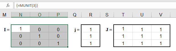
A simple way to create an n x n ones matrix (J) is to multiply the identity matrix by 0 and add 1, like this:
{ =1+0*MUNIT(n) }
The ones vector (j) of size n x 1 can be created by using INDEX to return the first column of the ones matrix, like this:
{ =INDEX(1+0*MUNIT(n),0,1) }
In older versions of Excel that don’t support the MUNIT function, you can create the ones vector, ones matrix and identity matrix using these formulas:
j =(1+0*ROW(INDIRECT("1:"&n)))
J =IF(ISERROR(OFFSET(INDIRECT("A1"),0,0,n,n)),1,1)
I =IF( ROW(OFFSET(INDIRECT("A1"),0,0,n,n)) = COLUMN(OFFSET(INDIRECT("A1"),0,0,n,n)), 1, 0)
Repeating Rows or Columns to Create a Matrix
Sometimes you may need to form a matrix by repeating a row or column. This can be done using MMULT and the ones vector.
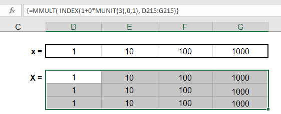
If you want to create a matrix with n rows by repeating row={1, 2, 3}, use the array formula =MMULT(j,row) where j is size n x 1.
{ =MMULT( INDEX(1+0*MUNIT(n),0,1), row) }
If you want to create a matrix with k columns by repeating col={1;2;3}, use the array formula =MMULT(col,TRANSPOSE(j)) where j is size k x 1.
{ =MMULT(col, TRANSPOSE(INDEX(1+0*MUNIT(k),0,1)) ) }
ROW or COLUMN Sums using the ONES Vector
It turns out that the ONES vector is very important in statistics for performing a very simple matrix operation: summing the rows or columns. Let’s say you have a range of size n (rows) x k (columns). You could either use the SUM function separately for each row or column, or you could use array formulas.
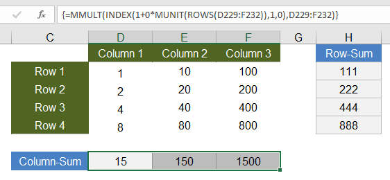
Column-Sum: To the sum the values within each COLUMN of the matrix and return the sums as a 1 x n array (or row vector), use
ones_vector =INDEX(1+0*MUNIT(ROWS(range)),0,1)
column_sum =MMULT(TRANSPOSE(ones_vector),range)
Row-Sum: To sum the values within each ROW of the matrix and return the sums as a k x 1 array (or column vector), use
ones_vector =INDEX(1+0*MUNIT(COLUMNS(range)),0,1)
row_sum =MMULT(range,ones_vector)
Creating a DIAGONAL Matrix
Element-wise multiplication of matrices can be used to create a Diagonal matrix. A Diagonal matrix is a special matrix where all of the off-diagonal terms are zeros. To create the Diagonal matrix, you multiply the matrix by the Identity matrix of the same size:
Diagonal =A*MUNIT(ROWS(A))
Many programs (but not Excel) include a function like diag(matrix) which returns an n x 1 vector containing the diagonal terms of an n x n matrix. To return the diagonal as a vector, you can use the row-sum operation on the Diagonal like this:
diag(A) =MMULT(A*MUNIT(ROWS(A)),(1+0*ROW(INDIRECT("1:"&ROWS(A)))))
Find the TRACE of a Square Matrix
The trace of a square matrix is just the sum of the diagonal elements. Therefore, the formula for calculating the trace is just:
trace(A) =SUM( A*MUNIT(ROWS(A)) )
Other Array Formula Examples
Linear Regression
The trend lines in an Excel chart allow you to do simple linear regression, but you can also do linear regression in Excel using matrix and array functions. It’s much easier to just use the LINEST function, but for fun I give the general formula for calculating the b matrix (the least squares estimators) when you have the y and X matrix. Or in other words, if you want to solve for b starting from y=Xb, you can do that using the formula b=(X‘X)-1X‘y which in Excel is:
{ =MMULT(MMULT(MINVERSE(MMULT(TRANSPOSE(x),x)),TRANSPOSE(x)),y) }
Alternate XNPV Function
If for some reason you don’t like Excel’s XNPV function or for some reason you need to use 360 days in a year instead of 365, you can use the following array formula in place of XNPV, where r is the discount rate.
{ =SUM(values_range/((1+r)^((date_range-INDEX(date_range,1))/365))) }
Running XIRR Formula
My Investment Tracker calculates an annualized compounded rate of return using a running XIRR array formula.
Some References for Array Formulas in Excel
- Guidelines and Examples of Array Formulas at support.office.com
- Array Formulas at cpearson.com — Some detailed information about using array formulas in Excel, along with some example array functions.
- Matrix Functions in Excel at bettersolutions.com — Examples showing the use of MDETERM, MINVERSE, MMULT, and TRANSPOSE.
- Using Excel to find Eigenvalues and Eigenvectors
- A.C.Rencher, Methods of Multivariate Analysis, John Wiley & Sons, Inc.: New York, 1995.