
Move or copy cells and cell contents
Use Cut, Copy, and Paste to move or copy cell contents. Or copy specific contents or attributes from the cells. For example, copy the resulting value of a formula without copying the formula, or copy only the formula.
When you move or copy a cell, Excel moves or copies the cell, including formulas and their resulting values, cell formats, and comments.
You can move cells in Excel by drag and dropping or using the Cut and Paste commands.

Move cells by drag and dropping
-
Select the cells or range of cells that you want to move or copy.
-
Point to the border of the selection.
-
When the pointer becomes a move pointer
 , drag the cell or range of cells to another location.
 , drag the cell or range of cells to another location.
Move cells by using Cut and Paste
-
Select a cell or a cell range.
-
Select Home > Cut
or press Ctrl + X. -
Select a cell where you want to move the data.
-
Select Home > Paste
or press Ctrl + V.
 or press Ctrl + X.
 or press Ctrl + V.
Copy cells by using Copy and Paste
-
Select the cell or range of cells.
-
Select Copy or press Ctrl + C.
-
Select Paste or press Ctrl + V.
Need more help?
You can always ask an expert in the Excel Tech Community or get support in the Answers community.
See Also
Move or copy cells, rows, and columns
Need more help?
Want more options?
Explore subscription benefits, browse training courses, learn how to secure your device, and more.
Communities help you ask and answer questions, give feedback, and hear from experts with rich knowledge.
How to Copy and Paste in Excel – Step-By-Step (2023)
Copy/pasting is something we have all known for ages now. But there’s so much more to the dynamic copy-paste tool of Excel than simple copying/pasting of values.
And the guide below will show you how resourceful the copy-and-paste tool of Excel can be. So let’s dive right in👇
Hold on! Download our sample workbook here to tag along with the guide.
How to copy and paste into Excel
Unlike any other spreadsheet program, Excel offers a huge variety of options for copying/pasting data.
You can paste anything – formulas, formatting, values, transposed values, and whatnot🖌
And the best part is that you can access a single option from multiple places, offering extra ease of use. So how do you copy and paste values in Excel? Let’s see below
Generally, there are three 3️⃣ ways in which you can copy/paste your data once you select a cell.
1. The clipboard group
The Clipboard section contains all the functions you need to copy and paste values in Excel. It sits in the Home tab of the ribbon.

You can use the Scissors option to cut data and the Two Sheets option to copy the data✂
The Clipboard icon is the paste button that holds all the copied data. The Paint Brush icon below is known as the Format Painter, which lets you copy the formatting🖌
And the options don’t just end here – Click on the arrow in the bottom right corner to view more copy/paste options.
2. The right-click menu
You can access the context menu by right-clicking the cell you want to copy. The dropdown list will show you a bunch of options.

Select Copy to make a copy of the selected cell in the clipboard. Once you copy a cell, a continuously moving border will enclose it.
Pro Tip!
You can also use CTRL + C to copy the data. It is the most common keyboard shortcut used in Excel and is very efficient.
Simply select the cell and press CTRL + C.
Then, select the destined cell and press CTRL + V to paste the copied contents into it 🥂
After you’ve copied the cell, navigate to the destination cell and paste it.
To paste the cell contents, right-click on the destination cell. From the context menu, select the option “Paste”📃

3. The CTRL button
This method is quite similar to using CTRL + C, but not many people know it🤔
- Select the cell.
- Press the CTRL key.
- Hover over the cell until the plus sign appears.
- Hold and drag the cell to a new location.
- You get an exact copy of your original cell in the new location.
How to copy formulas only in Excel
So now we know the basics of copy-pasting in Excel.
But do you know how to copy and paste only formulas in Excel? We do it using a trick.
Let’s see an example below.
The data set we use below shows if the given condition is true or false.

The function running behind these boolean values is the AND function. You can access it from the Formulas Tab 💻

Now let’s say we want to add another row at the bottom and copy the formula above it.

An easy way is to:
- Copy the formula above by selecting any cell that contains the formula and press CTRL + C.
- Right-click the cell where you want to paste the formula. A dropdown list will appear with the paste section like this ⏬

- Click on the Paste Special commands option.
- From the Paste Special menu, select the Formulas and Number formatting option (hovering over the icons shows their names).
The formula will be pasted into the new cell, and the cell references will adapt accordingly.

Similarly, if you want to copy the formula to multiple cells, you can do it using the Paste Special dialog box 💭
Launch the Paste Special Dialog box using the shortcut keys Alt + E + S.

Simply select the Paste option you want to apply on the cell while pasting data. And since we are dealing with formulas, we will select the option “Formulas”.
How to make a copy of an Excel sheet
Making a copy of an Excel sheet may seem difficult with no options visible on the face of the worksheet. But believe us, it is just a click away.

Say, we want to make a copy of Sheet 1🧾
There are two ways to do this. First, use the right-click menu, and second, use the CTRL key.
The right-click context menu:
- Select the sheet you want to copy.
- Right-click the sheet and select the Move or Copy option.

- You will see a pop-up asking for the location and whether you want to create a copy.

- Check the option to Create a Copy.
What happens if you don’t check the option to create a copy🤔
Excel will remove the sheet from the present workbook. And move it to the destination workbook.
- Choose the pasting location from the To Book option.
- Click Ok.

- The subject worksheet appears in the chosen location💪
Using the CTRL key:
To copy a sheet using the Control key, follow the steps below:
- Select the sheet.
- Press the CTRL key.
- Drag the sheet to a new location to make its copy.
We have created a copy of Sheet 1 in the same book.

- A new file, Sheet 1 (2), appears on the Sheet tab.
Copy values not formula
It’s time we see how to copy only the values in Excel and not the underlying formulas.
From the dataset below, let’s copy the cell values only 🔢

To copy cell values, follow the steps below:
- Select the cell or the range of cells whose value is to be copied.
- Press Ctrl + C to copy the cell values.
- Go to the blank cells where you want to paste the selected range.
- Right-click the first cell and open the Paste Special dialog box.
- From the Paste Special options, select the Values option.
This tells Excel to paste the values of the copied cells only 🌟

- Click Okay. And there you go!

Values from the copied range appear in all the cells selected.
Note that Excel has pasted the exact values only. You can select the cell and view the formula bar to see that the values have no formulas to them.
Had you pasted them simply, Excel would have copied and adapted the formula of the copied cells for the destination cells as follows 😵

Shortcut to paste values
Oh, and there’s a very efficient shortcut to paste values in Excel too 💪
- Select the values to be copied.
- Press CTRL + C to copy them.
- Go to the destination cells to paste values. Select the first cell of the destination cell range.
- Press CTRL + Alt + V.
- Press V.

- Select Ok.
- You’d have the cell values pasted in Excel without any cursor movement 🖱
How to copy formatting
We have so far seen how to copy and paste formulas and values. Let’s now have a look at the copy-pasting of formatting.
Hint: It’s done the same way as formulas and values are copied/pasted✌
We are using the same data set for this example. And we want to paste the existing formatting to the new cells below.

To do so:
- Select the cells with the source formatting (the formatting that you want to copy) to copy them.
- Once copied, select the cell (or cells) where you want to paste the cell formatting🖱
- You can use the context menu to open the Paste Special dialog box and choose Formatting. Or press CTRL + Alt + V and then T to paste the formatting only.
The results look like this:

Note how Excel has pasted the format (including the font style and the font size) to the destined cells.
There is yet another way to copy cell formatting in Microsoft Excel – by using the Format Painter. We bet you didn’t see that coming😎
All you need to do is select the cells containing the source formatting. And click the Paintbrush icon on the ribbon to activate the Format Painter

With the format painter activated, select the cells where you want to paste the formatting.
And tada! The new cells are formatted like the source formatting.

Pro Tip!
If you want to paste the formatting to a single cell or a range of adjacent cells only, click on the format painter once. In this case, the format painter will deactivate after painting the format once.
But, if you want to apply the source formatting to multiple non-adjacent cells, double-press the Format Painter icon. Now the format painter will stay active until you manually deactivate it 🎨
That’s it – Now what?
In this article, we learned how to copy and paste values and formulas in Excel. We also saw how we could paste cell formatting to a range of cells in a few easy steps.
And even though this article covers most of the aspects of the copy-paste tool in Excel, there’s still so much to learn.
Like the three most important functions of Excel. The VLOOKUP, IF, and SUMIF functions.
To learn these functions (and more!), enroll in my 30-minute free email course today.
Kasper Langmann2023-01-19T12:05:51+00:00
Page load link
Копирование и вставка
- Подробности
- Создано 04 Сентябрь 2012
| Содержание |
|---|
| Буфер обмена операционной системы |
| Буфер обмена Microsoft Office |
| Копирование и вставка в Excel |
| Специальная вставка |
| Перетаскивание при помощи мыши |
В статье описываются возможности использования буфера обмена Windows и Microsoft Office, а также особенности копирования и вставки данных в Excel. Понимание и правильное использование этих операций позволяет существенно ускорить выполнение рутинных операций при обработке данных.
Буфер обмена операционной системы
В терминах информационных систем буфер обмена (англ. clipboard) — это общедоступная для разных приложений область оперативной памяти. Операционная система предоставляет низкоуровневый программный интерфейс для перемещение данных в и из буфера обмена по запросу пользователя. Корректное применение этого программного интерфейса является стандартом при разработке Windows-приложений. То есть, любая программа должна предоставлять пользователю возможности использования буфера обмена при использовании одних и тех же сочетаний клавиш или пунктов меню. Далее будем говорить о Windows, хотя, в принципе, описание принципа работы буфера обмена идентично для любой современной операционной системы персональных компьютеров или мобильных устройств.
Копирование и вставка являются стандартными операциями для всех Windows-приложений. Для этого зарезервированы универсальные комбинации горячих клавиш, доступные практически в любой программе:
- Ctrl+c – скопировать (англ. copy)
- Ctrl+x – вырезать (англ. cut)
- Ctrl+v – вставить (англ. paste)
Часто также упоминаются аналогичные по функциональности сочетания клавиш: Ctrl+Ins – скопировать, Shift+Ins – вставить, Shift+Del – вырезать. Однако, мы не рекомендуем использовать эти сочетания, так как некоторые приложения заменяют их стандартное поведение на другое. Например, нажатие Shift+Del в Проводнике Windows вместо ожидаемого вырезания перемещаемого файла вызовет его удаление в обход корзины. То есть вместо перемещения может случиться безвозвратная потеря данных.
Если вы предпочитаете использовать мышь вместо клавиатуры, то стандартные поля ввода Windows-приложений обычно поддерживают контекстное меню с операциями копирования, вырезания и вставки текста.
Скопированный текст или другой блок данных может быть вставлен в другое приложение, в зависимости от возможностей последнего. Например, скопированный в Блокноте текст не получится затем вставить в графический редактор Paint. Однако же, тот же текст, набранный в Word, успешно вставляется в Paint в виде точечного рисунка. Такая возможность реализуется на программном уровне за счет перемещения данных в буфер обмена в нескольких форматах одновременно. Если набрать в Word полужирным шрифтом слово Example, затем его скопировать, то в буфере обмена появится несколько блоков информации:
| Example | Текст как набор символов без форматирования |
|
Example |
Текст с форматированием в формате HTML |
| {rtf1ansiansicpg1252uc1 {b Example}{par }} | Текст с форматированием в формате RTF |
| |
Точечный рисунок блока экрана |
Теперь, если попытаться вставить данные в Блокнот, то программа выберет из буфера обмена единственный доступный для себя вариант информации – текст без форматирования. Если то же самое сделать в Paint’е, то будет обработана последняя область – рисунок. Набор доступных форматов для копирования и вставки зависит от возможностей конкретной программы. Если приложение поддерживает несколько форматов информации (рисунки, текст, сложные объекты), то оно позволяет выбрать вариант вставки. Например, в Microsoft Word эта процедура реализована через пункт меню Специальная вставка:

Если использовать обычную вставку данных, то автоматически будет выбираться самый подходящий для этой программы формат. Excel также поддерживает операцию вставки данных в различных форматах по принципу Word, если информация в буфер обмена попала из другого приложения. Если же копирование диапазона ячеек было проведено в том же приложении, то специальная вставка заменяется внутренней операцией Excel (раздельная вставка значений, формул, форматов и пр.), при которой не задействуется буфер обмена операционной системы.
Некоторые другие приложения также реализуют собственные процедуры работы на основе операций копирования и вставки, не задействуя для этого буфер обмена. Так, например, в Проводнике операция «копировать» не перемещает весь файл в буфер обмена Windows. Вместо этого запоминается только ссылка на этот файл, которая будет обработана при выполнении операции вставки.
Буфер обмена Microsoft Office
Как уже отмечалось выше, за операции со стандартным буфером обмена отвечает операционная система. Одной из задач при этом является корректное использование оперативной памяти. Операционная система, в частности, заботится о своевременной очистке области буфера обмена. В текущей реализации стандартный буфер обмена Windows позволяет хранить только один блок скопированной информации. При вызове процедуры нового копирования этот блок предварительно очищается, а зарезервированная за ним область памяти становится доступной для использования в качестве буфера обмена.
Для улучшения возможностей работы с пользовательским интерфейсом в Microsoft Office, начиная с версии 2000 (9.0), реализован расширенный буфер обмена с возможностью одновременного хранения нескольких (до 24х) скопированных блоков информации. Пользователю предоставляется интерфейс выбора и вставки любого из этих блоков в любое открытое приложение Office (Excel, Word, PowerPoint, OneNote и др.). Возможно, более логично было бы реализовать подобную функциональность на уровне операционной системы (Windows), хотя это и потребует изменения стандартов для всех приложений. Сейчас получается, что множественный буфер обмена работает до тех пор, пока открыто хотя бы одно приложение Office. Если оно закрывается, то становится доступным только буфер обмена Windows с единственным блоком скопированной информации.
Интерфейс множественного буфера обмена в Office 2010 открывается и настраивается на ленте «Главная» в одноименном блоке (стрелка в нижнем правом углу).

Если говорить о полезности и удобстве работы с множественным буфером обмена, то здесь имеются различные мнения. Я лично никогда не использую эту функциональную возможность – проще еще раз скопировать. Но, скорее всего, это сила привычки.
Копирование и вставка в Excel
Как уже отмечалось, Excel полностью поддерживает буфер обмена Office, но, кроме того, в этой программе поддерживаются собственные операции копирования и вставки без использования буфера обмена.
Здесь следует заметить, что повторное использование объектов через копирование и вставку является одним из определяющих факторов ускорения обработки информации при использовании электронных таблиц Excel.
Что же в действительности происходит в Excel при нажатии кнопки «копировать» при выделении диапазона ячеек?
Во-первых, как и в прочих Windows-приложениях, набор информации помещается в буфер обмена операционной системы в нескольких форматах: простой текст, форматированный текст, точечный рисунок и др. Таким образом, вы, например, можете воспользоваться графическим редактором и вставить туда экранное отображение блока выделенных ячеек. Если вставить этот же блок обратно в Excel, то вставится рисунок:
Во-вторых (и это главное), при копировании Excel выполняет внутреннюю операцию для работы с ячейками электронной таблицы. По нажатию сочетания клавиш Ctrl+C, пункта контекстного меню либо кнопки копирования в памяти сохраняются ссылки на выделенные ячейки. Этих ячеек может быть огромное количество. Они могут располагаться одном прямоугольном диапазоне, либо в нескольких несвязанных диапазонах (для выделения таких диапазонов надо при выделении мышью удерживать клавишу Ctrl). Теоретически имеется возможность копирования ячеек на разных листах (несколько листов можно выделять также через удержание клавиши Ctrl на ярлыке листа), но эти ячейки должны располагаться по одному и тому же адресу, при этом последующая вставка возможна также только на этих же выделенных листах. На практике лучше отказаться от копирования-вставки на нескольких листах одновременно, так как эта операция не очень наглядна и часто приводит к потере данных.
Доступно также копирование ссылок между разными, но открытыми в одном приложении Excel, файлами. Типичной ситуацией, вызывающей непонимание со стороны пользователя, является обработка данных в нескольких одновременно открытых приложениях Excel. При попытке скопировать данные из одного файла в другой программа вставляет результат только в виде отформатированных значений без формул. Это не ошибка, просто несколько одновременно открытых программ Excel занимают различные области памяти и никаких ссылок между ними быть не может. При копировании и вставке в этом случае используется только буфер обмена Office. Для исправления ситуации откройте файлы в одном приложении Excel.


Еще раз обращаем внимание, что при запуске операции копирования, в память программы записываются не данные (текст, формулы, форматы), а только ссылки на адреса выделенных ячеек. Для наглядности интерфейс Excel обводит скопированные ячейки анимированной рамкой.
После копирования диапазонов становится доступной операция вставки. Перед этим необходимо выделить один или несколько диапазонов или ячеек для приема данных из скопированной области.
Вставка доступна до тех пор, пока пользователь не произвел действий, приводящих к изменению данных электронной таблицы. Можно выделять ячейки и диапазоны, перемещаться между листами и файлами. Также не отменяет область копирования сама операция вставки. Это позволяет копировать ячейки несколько раз подряд для разных диапазонов. Любые другие операции с пользовательским интерфейсом, например, ввод данных, группировка, сортировка, форматирование, приводят к сбросу скопированной ранее ссылки. Принудительно сбросить область копирования можно по нажатию клавиши Esc.
Если выделенная перед вставкой область листа не совпадает с размером скопированной области, то Excel попытается распространить данные несколько раз или вставить только часть данных. В некоторых случаях это бывает невозможно (например, области копирования и вставки пересекаются), тогда программа выдает сообщение об ошибке.
Кроме простой вставки, скопированный диапазон может быть добавлен в область листа с расширением границ влево или вниз через пункт контекстного меню «Вставить скопированные ячейки».
Если для вставки данных воспользоваться буфером обмена Office, то будут добавлены данные с потерей формул аналогично примеру с копированием между разными приложениями Excel.
По умолчанию при вызове операции вставки на выделенный диапазон будут распространены все атрибуты исходного диапазона, а именно: формула, формат, значение, примечание, условия. Иногда приводится сложное описание правил копирования формул, так как они вроде бы автоматически преобразуются при изменении адресов диапазона-приемника. На самом деле формулы копируются в формате R1C1 и при этом остаются неизменными (можете проверить, переключив вид листа Excel в R1C1). Отображение в привычном A1-формате просто преобразует формулу в новых координатах.
Операция «вырезания», в отличие от копирования, очищает исходный диапазон после проведения вставки. Если вставка не была выполнена, то никаких действий произведено не будет.
Специальная вставка
Другой важной особенностью копирования диапазонов Excel является раздельная вставка атрибутов скопированных диапазонов. В частности, можно вставить в новое место рабочего листа только комментарии из скопированного диапазона. Набор атрибутов, доступный для раздельного копирования, отображается в диалоге специальной вставки:
- значение
- формат
- формула
- примечание
- условия на значение (проверка данных)


В разных версиях Excel набор элементов специальной вставки немного отличается. Но независимо от этого можно воспользоваться повторной операцией вставки атрибута. Например, для вставки формул с примечаниями, но без форматов, надо скопировать один раз исходный диапазон, а затем последовательно выполнить две специальных вставки на одном и том же диапазоне: вставка только формул, затем вставка только примечаний.
Диалог специальной вставки содержит также блок переключателей, позволяющий производить математические операции над диапазоном данных: сложить, вычесть, умножить и разделить. Операция будет применена к диапазону, выделенному перед вставкой. А скопированные ячейки при этом будут содержать коэффициенты сложения, вычитания, умножения или деления. В большинстве случаев применяют единый коэффициент на весь диапазон. Например, можно скопировать число 10, затем выделить диапазон и выбрать специальную вставку с умножением – в результате все данные выделенного диапазона будут умножены на 10. Если в ячейках содержалась формула, то она будет преобразована по математическим правилам:


Еще одна возможность специальной вставки – это транспонирование диапазона. После выполнения этой операции результирующий диапазон будет повернут на 90 градусов – данные из строк попадут в столбцы и наоборот.
Настоятельно рекомендуем освоить и применять на практике специальную вставку – это незаменимая функция при разработке сложных финансовых моделей.
Как только была выполнена какая-то операция с данными электронной таблицы, либо в буфер обмена Office попала новая порция информации, воспользоваться ссылкой для вставки формул не получится. На картинках пример, показывающий такое поведение:
- в Excel копируется диапазон с формулами
- копируется какие-то данные в другом приложении (например, в Блокноте)
- при попытке вставить формулы в Excel данные будут вставлены только в качестве значений. Т.е. ссылка на формулы уже потеряна.


Перетаскивание при помощи мыши
Начинающие пользователи Excel быстрее всего осваивают копирование данных через перетаскивание ячеек. Для этого имеется специальный указатель на рамке выделенного диапазона. Кстати, эту возможность можно отключить в общих параметрах Excel.
Операция перетаскивания ячеек при помощи мыши в большинстве случаев является аналогом копирования и вставки для смежных диапазонов ячеек. С технической точки зрения основное отличие заключается в том, что при перетаскивании мыши никакие данные в буфере обмена не сохраняются. Excel выполняет только внутреннюю процедуру вставки, после чего очищает информацию об источнике копирования. С точки зрения пользовательского интерфейса отличительной особенностью перетаскивания является возможность заполнения ячеек на основе автоматически определяемого числового ряда в выделенном диапазоне. Многие думают, что Excel умеет продолжать только последовательно возрастающий ряд, прибавляя единицу. Это не так, программа сама формирует коэффициент увеличения как среднее значение в выделенном диапазоне. На картинках примера это число 2.


Если во всех выделенных ячейках перед началом перетаскивания содержатся формулы, то процедура будет полностью идентична операциям копирования и вставки. Кроме того, используя специальный указатель, можно явно запустить операцию копирования без изменения значений (опция «Копировать ячейки»):

Можно сказать, что перетаскивание на небольших диапазонах данных выполняется быстрее, но в общем случае операции копирования-вставки имеют более гибкие возможности.
Смотри также
» Использование Excel в задачах финансового менеджмента
В статье представлен обзор популярных задач финансового менеджмента, доступных для решения с помощью электронных таблиц. Выводы и…
» Уровни подготовки пользователей
В требованиях к офисным сотрудникам часто упоминается фраза «опытный пользователь Excel». Это же все пишут в своих резюме. И,…
» Основные принципы оптимизации работы в электронных таблицах
Знание специальных приемов работы в электронных таблицах Excel позволяет в разы сократить время разработки моделей, повысить…
» Надстройки Excel
Те, кто программирует на VBA для Excel, в определенный момент задумываются над распространением своих приложений в качестве независимых…
Copying and pasting is a very frequently performed action when working on a computer. This is also true in Excel.
It’s so common that almost everyone knows the keyboard shortcuts to copy Ctrl + C and paste Ctrl + V.
When using this in Excel, it will copy everything including values, formulas, formatting, comments/notes, and data validation.
This can be frustrating as sometimes you’ll only want the values to copy and not any of the other stuff in the cells.
In this post, you’ll learn all the ways to copy and paste only the values from your Excel data.
Example Data
The example data used in this post contains various formatting.
- Cell formatting such as font color, fill color, number formatting, and borders.
- Notes.
- SUM formula.
- A data validation dropdown list.
Paste Special Keyboard Shortcut
If you want to copy and paste anything other than an exact copy, then you’re going to need to become familiar with paste special.
A favorite method to use this is with a keyboard shortcut.
To use the paste special keyboard shortcut.
- Copy the data you want to paste as values into your clipboard.
- Choose a new location in your workbook to paste the values into.
- Press Ctrl + Alt + V on your keyboard to open up the Paste Special menu.
- Select Values from the Paste option or press V on your keyboard.
- Press the OK button.
This will paste your data without any formatting, formulas, comments/notes, or data validation. Nothing but the values will be there.
Paste Special Legacy Keyboard Shortcut
This keyboard shortcut is a legacy shortcut from before the Excel ribbon command existed and it’s still usable.
In fact, when you try and use this you’ll be greeted with the above warning to let you know this is from an earlier version of Microsoft Office.
When you have a range of data copied to your clipboard, you can open up the Paste Special menu by pressing Alt + E + S on your keyboard.
Once the Paste Special menu is open you can then press V for Values.
One advantage the legacy shortcut has is it can easily be performed with one hand!
Paste Special Values Keyboard Shortcut
Pasting as values is a very common activity in Excel. Because of this, a new keyboard shortcut was introduced to Microsoft 365 users for this exact purpose.
Press Ctrl + Shift + V on your keyboard to paste the last item in your clipboard as values.
This is the most useful new shortcut as it bypasses the paste special menu entirely.
Paste Special from the Home Tab
If you’re not a keyboard person and prefer using the mouse, then you can access the Paste Values command from the ribbon commands.
Here’s how to use Paste Values from the ribbon.
- Select and copy the data you want to paste into your clipboard.
- Select the cell you want to copy the values into.
- Go to the Home tab.
- Click on the lower part of the Paste button in the clipboard section.
- Select the Values clipboard icon from the paste options.
The cool thing about this menu is before you click on any of the commands you will see a preview of the data you’re about to paste. This makes it easy to ensure you’re selecting the right option.
Paste Values with Hotkey Shortcuts
Since the paste values command is in the ribbon, that also means you can access it with the Alt hotkeys.
Notice when you press the Alt key, the ribbon lights up with all the accelerator keys available.
Pressing Alt ➜ H ➜ V ➜ V will activate the paste values command.
Paste Values from Right Click Menu
Paste Values is also available from the right-click menu.
Copy the range of cells you want to paste as values ➜ right click ➜ select the paste values clipboard icon.
Paste Values with Quick Access Toolbar Command
If it’s a command you use quite frequently, then why not put it in the quick access toolbar?
This way it’s only a click away at all times!
Depending on where in the quick access toolbar you place it, it will also get its own easy to use Alt hotkey shortcut too.
Check out this post for details on how to add commands to the quick access toolbar, or this post on other interesting commands you can add to the quick access toolbar.
You can add the paste values command from the Excel Options screen.
- Select All Commands from the dropdown list.
- Locate and select Paste Values from the options. You can press P on your keyboard to quickly navigate to commands starting with P.
- Press the Add button.
- Use the Up and Down arrows to change the ordering of commands in your toolbar.
- Press the OK button.
The command will now be in your quick access toolbar!
If you place it in the 4th position like in this Example, then you can you Alt + 4 to access it with a keyboard shortcut.
Paste Values Mouse Trick
There’s a mouse option you can use to copy as values which most people don’t know about.
- Select the range of cells to copy.
- Hover the mouse over the active range border until the cursor turns into a four directional arrow.
- Right-click and drag the range to a new location.
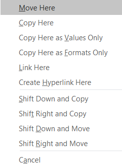
- When you release the right click, a menu will pop up.
- Select Copy Here as Values Only from the menu.
This is such a neat way, and there are a few other options in this hidden menu that are worth exploring.
Paste Values with Paste Options
There’s another sneaky method to paste values.
When you do a regular copy and paste, a small icon will appear in the bottom right corner of the pasted range. It will remain there until you interact with something else in your spreadsheet.
These are the paste options and you can click on it or press Ctrl to expand the options menu.
When you open the menu, you can then either click on the Values icon or press V to change the range into values only.
Paste Values and Formulas with Text to Columns
I don’t really recommend using this method, but I’m going to add it just for fun.
A few caveats with this method.
- You can only copy and paste one column of data.
- It will keep any formulas.
- It will remove the formatting, comments, notes, and data validation.
If that’s exactly what you’re looking for, then this method might be of interest.
Select a single column of data ➜ go to the Data tab ➜ select the Text to Column command.
This will open up the Convert Text to Column Wizard. In the first step, you can select Delimited and press the Next button.
You can also select Fixed width as we won’t be using the text to column functionality it doesn’t really matter.
In the next step, remove any selected delimiters and press the Next button.
In the last step, select the destination cell for the output and press the Finish button.
You can see the results have all the formatting gone but any formulas still remain.
Paste Values with Advanced Filters
This one is another not-quite paste values option and is listed for fun as well.
It will remove any formulas, comments, notes, and data validation but will leave all cell formatting.
With your data selected go to the Data tab then select the Advanced command in the Sort and Filter section.
From the Advanced Filter Menu.
- Select Copy to another location.
- Leave the Criteria range empty.
- Select a location to place the copied data.
- Press the OK button.
This will create a copy of the data as values and remove any formulas, comments, notes, and data validation.
You can then remove the cell formatting that’s left by going to the Home tab ➜ Clear ➜ and selecting the Clear Formats option.
Conclusions
Wow! That’s a lot of different ways to paste data as values in Excel.
It’s understandable there are so many options given it’s an essential action to avoid carrying over unwanted formatting.
You’re eventually going to need to do this and there are quite a few ways to get this done.
What’s your favorite way? Did I miss any methods you use? Let me know in the comments!
About the Author
John is a Microsoft MVP and qualified actuary with over 15 years of experience. He has worked in a variety of industries, including insurance, ad tech, and most recently Power Platform consulting. He is a keen problem solver and has a passion for using technology to make businesses more efficient.
Copy Paste is the most common action when you start to work with Excel.
Benefits of the action Copy Paste
With Excel, you can copy any cell or any range of cell
- Select the cell you want to copy and click on the following icon «Copy» in the Home tab.
- Just after you see an animation with dotted lines moving (the dancing ants 😉) This indication means that the cell has been copied in the contain of the cell is in the memory of the computer.
- Then, select the cell where you want to paste the contain of the first cell
- Click on the Paste icon.
- All the contain of the first cell (color, font, borders, formula) is transferred to the second cell.

Keyboard Shortcut
You can also use the following shortcut to perform the same action
| Copy contents of the selection to the clipboard | Ctrl + C |
| Paste contents of the clipboard. | Ctrl + V |
The fill-handle
When you want to copy / paste on adjacent cells, it is faster to do this action with the mouse. In the bottom-right corner of a cell, you notice a square: it’s the fill-handle.
Whatever the contained of your original cell you just have to click and drag to copy this cells.

If you have a single value, use the fill-handle will copy the same value. If you press Ctrl, you extend the series.
Increase series automatically
The fill-handle helps you to increase series of values automatically. NO FORMULA needed 😉
Duplicate column with the Ctrl Key
If you want to duplicate a column, the easiest way is to
- Select the column you want to duplicate
- Move the cursor to the edge of the selection
- Press the Ctrl key
- Drag and Drop BUT never release the Ctrl Key

Copy a formula
When the cell contains a formula, Excel automatically changes the references of the formula.
Let’s copy cell C2 to the range C3:C6.

Automatically, Excel has changed the references of the cells in the formulas 😉
You can «block» the cell references by putting the $ sign on both sides of the reference to ensure that references do not move. To avoid mistake with the reference of the cells, refer to this article.
Tutorial video with all the tricks
If you want to know more tricks with the copy-paste, have a look at this video
Knowing how to copy and paste is one of the most basic things you can learn to do in Excel. And while everyone is familiar with doing it, you might be surprised that there are several ways to do it, some more common than others.
Using Ctrl + C and Ctrl + V
This is definitely one of the more common ways that people are familiar with copying and pasting. It simply involves selecting the cells you want to copy, pressing Ctrl + C, and then selecting where you want to paste them, and then clicking Ctrl+ V.
Using the mouse to right-click copy and paste

Also another one of the more common ways to copy and paste. Here you’ll select what you want to copy, right-click and select copy. Then, select where you want to paste the data, then click right-click and paste. This way avoids having to use the keyboard but requires pulling up the menu with two mouse clicks.
Using the mouse and keyboard together

Hold down Ctrl while selecting the cell that you want to copy and drag it to your destination. Then, release the mouse button and your data will be copied.
Note, if you release the Ctrl button first, and then release the mouse button, then you will have moved the cell (the equivalent of Ctrl + X, Ctrl+V) instead of copying it. The advantage of this method is you don’t have to click as much and it’s useful if you’re quickly copying within the same area. The disadvantage is this method won’t work if you want to copy the data onto another tab or workbook.
Using right-click to copy and paste

Select a cell and hover over the borders until you see a crosshair appear. Then hold down on right click and drag it to where you want to copy it to, then release the button. You’ll be left with many options, including copying the cell or moving it. Technically this involves a second click, but you only have to bring up the menu once.
Using VBA
This is obviously not a method I’d suggest if you wanted to just copy cells over one time unless it was part of a larger macro you’re working on. But to copy data over in VBA it’s a fairly straightforward process that includes just one line of code:
Range(“A1”).copy Range(“A2”)
The first range (A1) is the cell you’re copying and in the above example, A2 is where you’re pasting it to.
If you liked this post on How to Copy and Paste in Excel (5 Different Ways), please give this site a like on Facebook and also be sure to check out some of the many templates that we have available for download. You can also follow us on Twitter and YouTube.

Microsoft Excel is a fairly powerful tool due to the study it does with the data, this has led it to become a very popular software for the financial and accounting sector . It has improved intelligence, since it allows you to create and edit files, run graphics, make spreadsheets, optimize formulas and much more, in a very practical and simple way.
As in any program of Microsoft Office , sometimes there is a need to make a copy paste so as not to have to transcribe the information back to the destination location. So these actions over time have become essential for those who work with a computer, thus being automated instructions.
It has become so widespread that it became fundamental when composing and restructuring any document. If you still do not know how to do this, in this tutorial we will explain step by step the processes that you must do to be able to do it and fill with cells cells in Excel . We will also show you how to solve the problems when this has been blocked.
Steps and methods to copy and paste the contents of cells in Excel
The main objective of copy and paste is to save you time when manually writing a text. That is why we will detail below the different methods to do it from the different computer shortcuts. Discover all the Excel commands in this part .
Keyboard shortcuts for copy and paste
If you will do this repeatedly, it is best to look for a more comfortable way to do it without having to use the mouse. We will help you make the process even simpler than it already is, just by selecting the text you want. In this case the Ctrl key will be the protagonist of all shortcuts.
- Ctrl + C: This command is used to copy the cells you have selected to place them in another place or destination.

- Ctrl + X : It is manipulated to cut the chosen cells and proceed to save them to the clipboard.

- Ctrl + V : With this you will be able to paste the cells that are inside the clipboard group wherever you want.

From the options bar
Another way to execute it is through the options bar, there are all the elements that make up Excel, including the most basic ones such as copy, cut and paste . When you select the content you want, it is deposited in a buffer memory, called clipboard .
- The first thing you will have to do is select the “Start” option.
- Then, choose “Clipboard” and then proceed to click on “Copy”, to duplicate the cells or the chosen content .
- Once all the data has been copied, you must select the box where you want to move them and press “Start” > “Clipboard”> “Paste.”

Using drag and drop
With this type of method you do not need to be an expert in Excel , because it is quite fast and simple to manipulate, an alternative that allows you to perform this interface. You just need to select and slide to Where do you want the text attached?

- First you have to select the range of cells that you want to copy and cut.
- Press the left mouse button on your computer to limit the rank and then move it to its new position.
- Then, simply you will have to release the mouse button to the place where you want take the data.
- Finally you have to know that before releasing the mouse you must press the Ctrl key + click with the mouse.

From the fill controller
This type of method is the one that allows you to copy a set of data into continuous cells for ease. It is visualized with a small black box that is located in the lower right corner and that when placing the courses on it, changes to a cross.

- The first thing you should do is select the cell and fill in the adjacent ones.

- Double-clicking the fill controller will copy the selected range down to locate a cell with content.

- In this way the formula will be automatically copied with its respective calculation.

In the same way you can do it with this process, which allows you to achieve it quickly. You will only need to right-click your computer to see the context menu.
- Select the cells and click with the left button of the mouse on top of it.
- Then choose the option that indicates “Copy or cut ”.
- Choose the destination that you have decided to transfer the data.
- Again click the left mouse button, but this time to choose potentiallyPegar†.

How to copy and drag Excel formulas into another cell or spreadsheet ?
If for some reason you want to copy and drag Excel formulas to another column or spreadsheet, you can choose specific pastes in target cells.

- Choose the cell that has the formula that you want to copy.
- Click “Start” choose “Copy ” or use the shortcut Ctrl+C.
- Now, on the same or another sheet, you have to press and click on the cell in the one you want to place.
- In order to paste the formula with its format, you will have to click on “Start”> “Paste” or also with Ctrl + V.
How to solve the problem when Excel crashes when copying and pasting and not answer?
We have already seen all the steps and different methods that you should use to be able to copy and paste in Excel but, How can you do to solve the problem when the application crashes when trying to do it and does not respond? strong> Next we’ll mention how to solve it.
Test the recovery of MS Office applications span >
This option may allow you to save your documents when the program has this error, so you don’t lose what you have done. You will also be able to recover files that were not saved at the indicated time.
- Go to the “Start” menu of your computer > “ All programs “> “Tools Microsoft Office “ >” MS Office application recovery. “
- Now you must select the document that does not respond. li>
- Then click on “Recover application” and rescue the document.
Using the Microsoft Office self-recovery
Previously Excel had a Autosave option, but for a few years this was supplanted by self-recovery. This causes the documents made in this interface to be saved with a backup copy. So if they close unexpectedly, it recovers the file:

- Go to “File” then “Information” and then “Manage versions”. There you can examine the backup copies of the unsaved files.
- Locate the Excel workbook and click where it says “Open” and ” Save ”.
When working with large amounts of data in Excel, you might find the need to copy and paste something that you’ve already written, or perhaps wholly move a selection. Whether you are working with data within a single worksheet, multiple worksheets, or even various workbooks, there are easy shortcuts you can use the cut, copy, and paste.
These instructions apply to Excel 2019, 2016, 2013, 2010, and Excel for Microsoft 365.
Copying Data in Microsoft Excel
Copying data in Excel is convenient when you need to duplicate functions, formulas, charts, and other data. The new location can be on the same or different worksheet or even in a completely different workbook.
As in all Microsoft programs, there is more than one way of accomplishing a task. In Excel, you can copy and move data in three ways:
- Using a keyboard shortcut.
- Using the right-click context menu.
- Using menu options on the Home tab of the ribbon.
When the copy command is activated, the clipboard temporarily stores a duplicate of the selected data until you paste it into the destination cell or cells.
Other methods of copying data that don’t involve using the clipboard include using the fill handle and drag and drop with the mouse.
Copy and Paste Data in Excel With Shortcut Keys
The easiest way to cut, copy, and paste, arguably, is with keyboard shortcuts. The keyboard key combinations for copying and pasting data are:
Ctrl + C — activates the copy command
Ctrl + V — activates the paste command
- Click a cell or multiple cells to highlight them.
- Press and hold down the Ctrl key on the keyboard.
- Press and release the C key without releasing the Ctrl key.
- A moving border (sometimes called marching ants) will surround the selected cell(s).
- Click the destination cell — when copying multiple cells of data, click the cell in the top left corner of the destination range.
- Press and hold down the Ctrl key on the keyboard.
- Press and release the V key without releasing the Ctrl key.
- The duplicated data should now be in both the original and destination locations.
The arrow keys on the keyboard can be used instead of the mouse pointer to select both the source and destination cells when copying and pasting data.
- To select multiple adjacent cells with the arrow keys, press and hold down the Shift key.
- To select multiple non-adjacent cells with the arrow keys, use the Ctrl key.
Copy Data in Excel With the Context Menu
While the options available in the context menu, or right-click menu, usually change depending upon the object selected, the cut, copy and paste commands are always available.
- Click on a cell or multiple cells to highlight them.
- Right-click on the selected cell(s) to open the context menu.
- Choose copy from the available menu options.
- A moving black border will surround the selected cell(s).
- Click on the destination cell — when copying multiple cells of data, click on the cell in the top left corner of the destination range.
- Right-click on the selected cell(s) to open the context menu.
- Choose paste from the available menu options.
- The duplicated data should now be in both the original and destination locations.
Copy Data With the Ribbon
The copy and paste commands are in the Clipboard section on the left-hand side of the Home tab of the ribbon.
- Click on a cell or multiple cells to highlight them.
- Click on the Copy icon on the ribbon.
- A moving black border will surround the selected cell(s).
- Click on the destination cell — when copying multiple cells of data, click on the cell in the top left corner of the destination range.
- Click on the Paste icon on the ribbon.
- The duplicated data should now be in both the original and destination locations.
Moving Data in Microsoft Excel
There is no move command in Excel. To move data, you need to cut and paste it from one location to the new one. You can use cut/paste in Excel to relocate functions, formulas, charts, and other data. The new location can be in the same or different worksheet or even in a completely different workbook.
As with copying, there are three ways to cut data in Excel:
- Using a keyboard shortcut.
- Using the right-click context menu.
- Using menu options on the Home tab of the ribbon.
When you cut data in Excel, the clipboard temporarily stores it, just like when you copy data.
Move Data in Excel With Shortcut Keys
The keyboard key combinations used to copy data are:
Ctrl + X — activates the cut command
Ctrl + V — activates the paste command
- Click on a cell or multiple cells to highlight them.
- Press and hold down the Ctrl key on the keyboard.
- Press and release the X without releasing the Ctrl key.
- A moving black border will surround the selected cell(s).
- Click on the destination cell — when moving multiple cells of data, click on the cell in the top left corner of the destination range.
- Press and hold down the Ctrl key on the keyboard.
- Press and release the V key without releasing the Ctrl key.
- The selected data should now be in the destination location only.
The arrow keys on the keyboard can be used instead of the mouse pointer to select both the source and destination cells when cutting and pasting data.
- To select multiple adjacent cells with the arrow keys, press and hold down the Shift key.
- To select multiple non-adjacent cells with the arrow keys, use the Ctrl key.
Move Data in Excel With the Context Menu
When you right-click on a cell, the context menu always includes the cut, copy, and paste commands.
- Click on a cell or multiple cells to highlight them.
- Right-click on the selected cell(s) to open the context menu.
- Choose cut from the available menu options.
- A moving border (sometimes called marching ants) will surround the selected cell(s).
- Click on the destination cell — when copying multiple cells of data, click on the cell in the top left corner of the destination range.
- Right-click on the selected cell(s) to open the context menu.
- Choose paste from the available menu options.
- The selected data should now be only in the destination location.
Move Data in Excel With the Ribbon
The cut and paste commands are in the Clipboard section on the Home tab of the ribbon.
- Click on a cell or multiple cells to highlight them.
- Click on the Cut icon on the ribbon.
- A moving black border will surround the selected cell(s).
- Click on the destination cell — when copying multiple cells of data, click on the cell in the top left corner of the destination range.
- Click on the Paste icon on the ribbon.
- The selected data should now be in the destination location only.
Thanks for letting us know!
Get the Latest Tech News Delivered Every Day
Subscribe
Copying and Pasting a cell or a range of cells is one of the most common tasks users do in Excel.
A proper understanding of how to copy-paste multiple cells (that are adjacent or non-adjacent) would really help you be a lot more efficient while working with Microsoft Excel.
In this tutorial, I will show you different scenarios where you can copy and paste multiple cells in Excel.
If you have been using Excel for some time now, I’m quite sure you would know some of these already, but there’s a good chance you’d end up learning something new.
So let’s get started!
Copy and Paste Multiple Adjacent Cells
Let’s start with the easy scenario.
Suppose you have a range of cells (that are adjacent) as shown below and you want to copy it to some other location in the same worksheet or some other worksheet/workbook.

Below are the steps to do this:
- Select the range of cells that you want to copy

- Right-click on the selection
- Click on Copy

- Right-click on the destination cell (E1 in this example)
- Click on the Paste icon
The above steps would copy all the cells in the selected range and paste them into the destination range.

In case you already have something in the destination range, it would be overwritten.
Excel also gives you the flexibility to choose what you want to paste. For example, you can choose to only copy and paste the values, or the formatting, or the formulas, etc.
These options are available to you when you right-click on the destination cell (the icons below the paste special option).
Or you can click on the Paste Special option and then choose what you want to paste using the options in the dialog box.
Useful Keyboard Shortcuts for Copy Paste
In case you prefer using the keyboard while working with Excel, you can use the below shortcut:
- Control + C (Windows) or Command + C (Mac) – to copy range of cells
- Control + V (Windows) or Command + V (Mac) – to paste in the destination cells
And below are some advanced copy-paste shortcuts (using the paste special dialog box).
To use this, first copy the cells, then select the destination cell, and then use the below keyboard shortcuts.
- To paste only the Values – Control + E + S + V + Enter
- To paste only the Formulas – Control + E + S + F + Enter
- To paste only the Formatting – Control + E + S + T + Enter
- To paste only the Column Width – Control + E + S + W + Enter
- To paste only the Comments and notes – Control + E + S + C + Enter
In case you’re using Mac, use Command instead of Control.
Also read: How to Cut a Cell Value in Excel (Keyboard Shortcuts)
Mouse Shortcut for Copy Paste
If you prefer using the mouse instead of the keyboard shortcuts, here is another way you can quickly copy and paste multiple cells in Excel.
- Select the cells that you want to copy
- Hold the Control key
- Place the mouse cursor at the edge of the selection (you will notice that the cursor changes into an arrow with a plus sign)
- Left-click and then drag the selection where you want the cells to be pasted

This method is also quite fast but is only useful in case you want to copy and paste the range of cells in the same worksheet somewhere nearby.
If the destination cell is a little far off, you’re better off using the keyboard shortcuts.
Copy and Paste Multiple Non-Adjacent Cells
Copy-pasting multiple cells that are nonadjacent is a bit tricky.
If you select multiple cells that are not adjacent to each other, and you copy these cells, you’ll see a prompt as shown below.

This is Excel’s way of telling you that you cannot copy multiple cells that are non-adjacent.
Unfortunately, there’s nothing that you can do about it.
There’s no hack or a workaround, and if you want to copy and paste these nonadjacent cells, you will have to do this one by one.
But there are a few scenarios where you can actually copy and paste non-adjacent cells in Excel.
Let’s have a look at these.
Copy and Paste Multiple Non-Adjacent Cells (that are in the same row/column)
While you can not copy non-adjacent cells in different rows and columns, if you have non-adjacent cells in the same row or column, Excel allows you to copy these.
For example, you can copy cells in the same row (even if these are non-adjacent). Just select the cells and then use Control + C (or Command + C for Mac). You will see the outline (the dancing ants outline).

Once you have copied these cells, go to the destination cell and paste these (Control + V or Command + V)
Excel will paste all the copied cells in the destination cell but make these adjacents.
Similarly, you can select multiple nonadjacent cells in one column, copy them, and then paste it into the destination cells.
Copy and Paste Multiple Non-Adjacent Rows/Columns (but adjacent cells)
Another thing Excel allows is to select non-adjacent rows or non-adjacent columns and then copy them.

Now when you paste these in the destination cell, these would be pasted as adjacent rows or columns.

Below is an example where I copied multiple non-adjacent rows from the dataset and pasted these in a different location.
Copy Value From Above in Non-Adjacent Cells
One practical scenario where you may have to copy and paste multiple cells would be when you have gaps in a data set and you want to copy the value from the cell above.
Below I have some dates in column A, and there are some blank cells as well. I want to fill these blank cells with the date in the last filed cell above them.

To do this, I would need to do two things:
- Select all the blank cells
- Copy the date from the above-filled cell and paste it into these blank cells
Let me show you how to do this.
Select All Blank Cells in the Dataset
Below are the steps to select all the blank cells in column A:
- Select the dates in column A, including the blank ones that you want to fill

- Press the F5 key on your keyboard. This will open the Go To dialog box.
- Click the Special button. This will open the Go To Special dialog box.

- In the Go To Special dialog box, select Blanks

- Click OK
The above steps would select all the blank cells in column A.

Now, we want to somehow copy the value in the above field cell in these blank cells. This cannot be done using any copy-paste method so we will have to use a formula (a very simple one).
Fill Blank Cells with Value Above
This part is really easy.
- With the blank cell selected, first hit the equal to key on your keyboard

- Now hit the Up arrow key. This will automatically enter the cell reference of the cell that is above the active cell.

- Hold the Control key and press the Enter key
The above steps would enter the same formula in all the selected blank cells – which is to refer to the cell above it.

While this is a formula, the end result is that you have the blank cells filled with the above-filled date in the data set.
Once you have the desired result, you can convert the formula into values if you want (so that the formula doesn’t update the cells in case you change any value in a cell that is being referenced in the formula).
So these are a couple of methods you can use to copy and paste multiple cells (adjacent and non-adjacent cells) in Excel. I am sure using these methods will help you save tons of time in your day-to-day work.
I hope you found this tutorial useful!
Other Excel tutorials you may also like:
- How to Copy and Paste Column in Excel? 3 Easy Ways!
- How to Copy Excel Table to MS Word (4 Easy Ways)
- How to Copy Conditional Formatting to Another Cell in Excel
- How to Copy and Paste Formulas in Excel without Changing Cell References
- How to Edit Cells in Excel?