
Column Header in Excel (Table of Contents)
- Introduction to Column Header in Excel
- How to Use Column Header in Excel?
Introduction to Column Header in Excel
Column Header is a very important part of excel as we work on different types of Tables in excel every day. Column Headers basically tell us the category of the data in that column to which it belongs. For example, if column A contains Date, then Column header for Column A will be “Date”, or suppose column B contains Names of the student, then column header for Column B will be “Student Name”. Column Headers are important in a way when a new person looks at your excel; he can understand the meaning of the data in those columns. It is also important because you need to remember how the data has been organized in your excel. So from the data organization standpoint, Column Headers play a very important role.
In this article, we will look at the best possible ways of how we can organize or format the column headers in excel. There are many ways of creating headers in excel. The three best possible ways of creating headers are below.
- Freezing Row/Column.
- Printing a header row.
- Creating a header in Table.
We will look at each way of creating a header one by one with the help of examples.
Suppose you are working on the data which has a large number of rows, and when you scroll down in the worksheet to look at some data, you may not be able to look at the Column Header. This is where Freeze Panes helps in excel. You can scroll down in the excel sheet without losing visibility to the column headers.
How to Use Column Header in Excel?
Column Header in Excel is very simple and easy. Let’s understand how to use the column Header in Excel with some examples.
You can download this Column Header Excel Template here – Column Header Excel Template
Example #1 – Freezing Row/Column
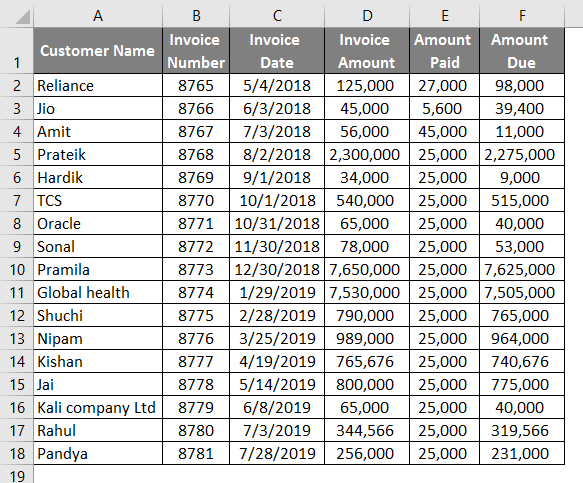
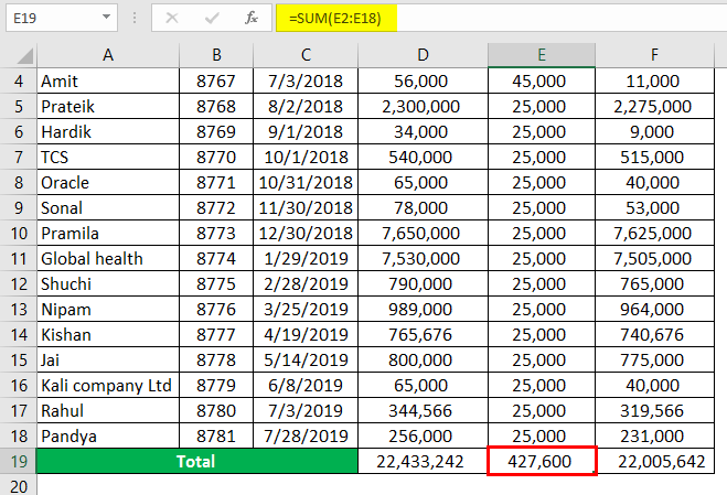
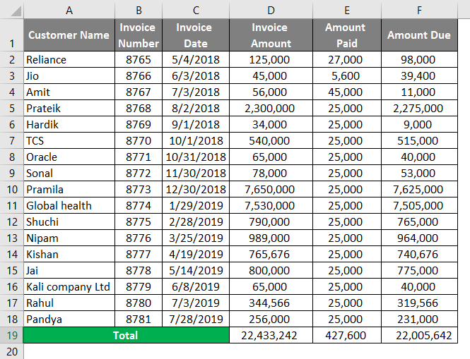
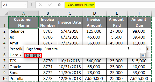
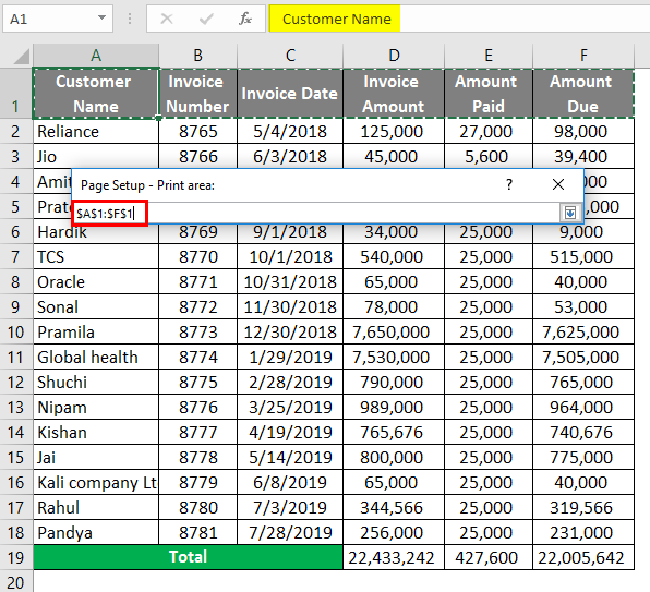
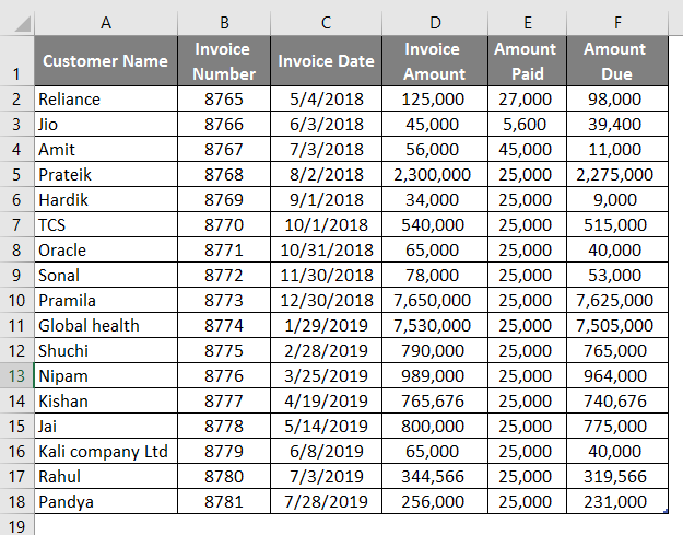
- Suppose there is data related to customers in excel, as shown in the below screenshot.
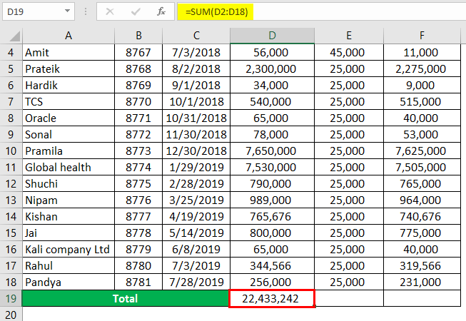
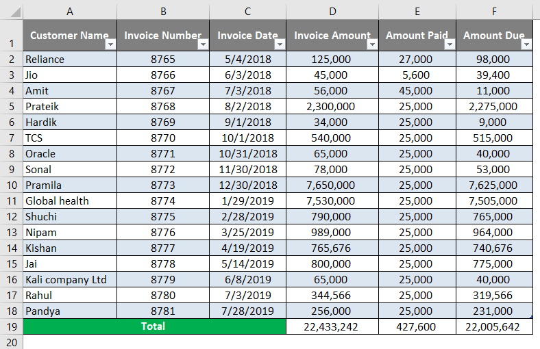
- Use SUM formula in cell D19.
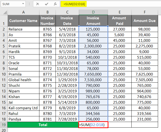
- After using the SUM formula, the output is shown below.
- The same formula is used in cell E19 and cell F19.
You need to follow the below steps to freeze the top row.
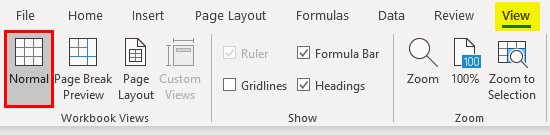
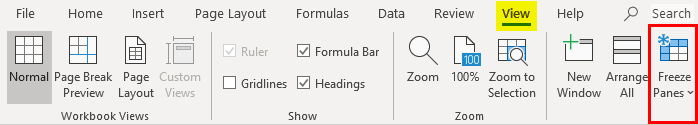
- Go to the View tab in Excel.
- Click on the Freeze Pane Option
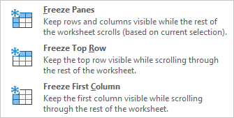
- You will see three options after clicking on the Freeze Pane option. You need to select the “Freeze Top Row” option.
- Once you click on the “Freeze Top Row”, the top row will be freezer, and you scroll down in excel without losing visibility to excel. You can see in the below screenshot that Row 1, which has column headers, are still visible even when you scroll down.
Example #2 – Printing a Header Row
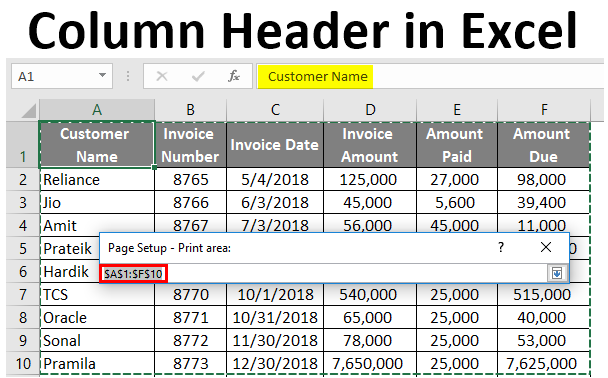
When you are working on large spreadsheets where data is spread across multiple pages and when you need to take a print out, it doesn’t fit well on one page. The printing job becomes frustrating as you are not able to see the column headers in print after the first page. In that scenario, there is a functionality in excel known as “Print Titles”, which helps set a row or rows to print at the top of every page. We will take a similar example which we have taken in Example 1.
Follow the below steps to use this functionality in Excel.
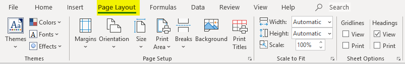
- Go to the Page Layout tab in Excel.
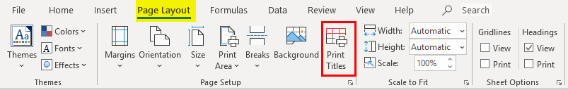
- Click on Print Titles.
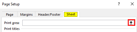
- After clicking on the Print Titles option, you will see the below window open for Page Set up in excel.
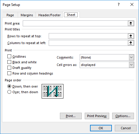
- In the Page Set up window, you will find different options that you can choose.
(a) Print Area
- To select Print Area, click on the button on the right side, as shown in the screenshot.
- After clicking on the button, the navigation window will open. You can select from Row 1 to Row 10 to print the first 10 rows.
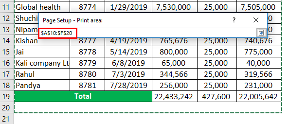
- If you want to print Row 11 to Row 20, you can select the Print Area as Row 11 to Row 20.
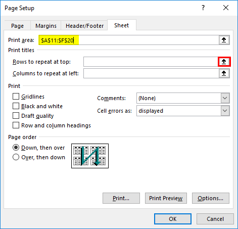
- Under Print Titles, you can find two options.
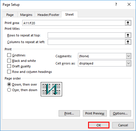
(b) Rows to Repeat at Top
This is where we need to select the column header, which we want to repeat on every page of the printout. To select Rows to repeat at the top, click on the button on the right side, as shown in the screenshot.
After clicking on the button, the navigation window will open. You can select Row 1, as shown in the below screenshot.
(C) Columns to Repeat at Left
This is the column that you want to see on the left, which will repeat on every page. We will keep it as blank as we don’t have any row headers in our table.
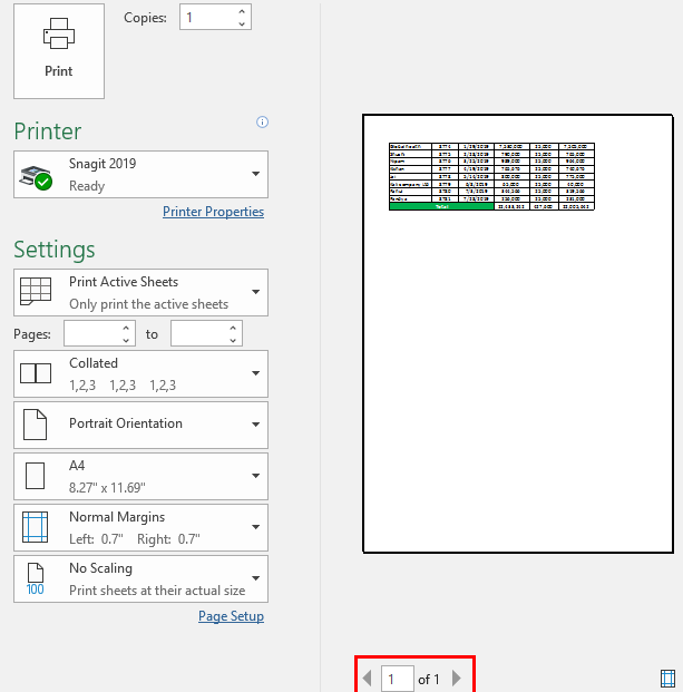
- Now click on the “Print Preview” option on the page setup as shown in the below screenshot to see the Print Preview. As you can see in the below screenshot, the print area is from Row 11 to Row 20, with the column headers in Row 1.
- Click on Ok in the Page setup window after exiting from Print Preview.
Example #3 – Creating a Header in a Table
One of the features in Excel is that you can convert your data into a Table. It automatically creates Headers when you convert your data into a table. But please take a note here that these headers are different from the Worksheet column heading or printed headers which we have seen earlier.
- We will take a similar example which we have taken earlier.
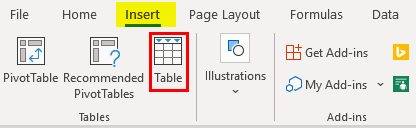
- Click on the “Insert” tab and then click on the “Table” button.
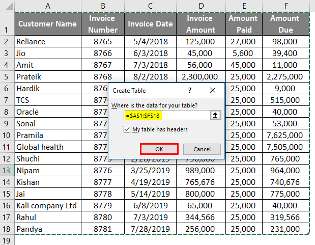
- After clicking on the “Table” option, you can give the range of data that you want to convert into the table and also select the checkbox of “My Table has Headers”, as shown in the below screenshot. The first row of your selection will automatically be assigned as column headers.
- Click Ok. You will see your data is converted into a Table.
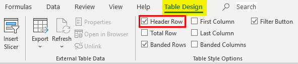
- You can Enable or Disable the Header row by going into the “Design” tab of the Table.
Things to Remember About Column Headers in Excel
- Always remember to format column headers differently and use Freeze panes to have visibility on the column header at all times. It will help you save time of scrolling up and down to understand data.
- Make sure to use the Print Area option and Rows to repeat at every page option while printing. This will make your printing job easy.
- Selection of Range and Column header is important while creating Table in Excel.
Recommended Article
This is a guide to Column Header in Excel. Here we discuss How to use Column Header in Excel along with practical examples and downloadable excel template. You can also go through our other suggested articles –
- Compare Two Columns in Excel for Matches
- Freeze Columns in Excel
- COLUMNS Formula in Excel
- Excel Header Row
Last Update: Jan 03, 2023
This is a question our experts keep getting from time to time. Now, we have got the complete detailed explanation and answer for everyone, who is interested!
Asked by: Harmony Towne
Score: 4.4/5
(37 votes)
In Excel and Google Sheets, the column heading or column header is the gray-colored row containing the letters (A, B, C, etc.) used to identify each column in the worksheet. The column header is located above row 1 in the worksheet.
How do I make column headings in Excel?
Open the Spreadsheet
- Open the Spreadsheet.
- Open the Excel spreadsheet where you want to define your column headings.
- Use the Page Layout Tab.
- Click the «Page Layout» tab at the top of the ribbon, then find the Sheet Options area of the ribbon, which includes two small checkboxes under the Headings category.
What makes column headings?
The information across the top makes up the column headers. The states make up the row headers. If someone is reading this table visually, it is the intersection of those labels that makes the data within the table make sense. … With no headers, starting at the same number «11» cell, the user has no context.
What are headers in Excel?
A header in excel: It is a section of the worksheet that appears at the top of each of the pages in the excel sheet or document. This remains constant across all the pages. It can contain information such as Page No., Date, Title or Chapter Name, etc.
Where are headings in Excel?
On the Insert tab, in the Text group, click Header & Footer. Excel displays the worksheet in Page Layout view. To add or edit a header or footer, click the left, center, or right header or footer text box at the top or the bottom of the worksheet page (under Header, or above Footer). Type the new header or footer text.
38 related questions found
What is AutoFilter in Excel?
Excel’s AutoFilter feature makes filtering out unwanted data in a data list as easy as clicking the AutoFilter button on the column on which you want to filter the data and then choosing the appropriate filtering criteria from that column’s drop-down menu.
Where is the center header section in Excel?
Click the Insert tab, and click Header & Footer. This displays the worksheet in Page Layout view. The Header & Footer Tools Design tab appears, and by default, the cursor is in the center section of the header.
What is a sheet name code in Excel?
In Excel. … Using the sheet name code Excel formula requires combining the MID, CELL, and FIND functions into one formula. For example, if you are printing out a financial model. Discover the top 10 types onto paper or as a PDF, then you may want to display the sheet name on the top of each page.
Why can’t I see my header in Excel?
The Advanced options of the Excel Options dialog box. Make sure the Show Row and Column Headers check box is selected. If cleared, then the header area is not displayed.
How do I create a header row in Excel?
Go to the «Insert» tab on the Excel toolbar, and then click the “Header & Footer” button in the Text group to start the process of adding a header. Excel changes the document view to a Page Layout view. Click on the top of your document where it says “Click to Add Header,” and then type the header for your document.
What do you call the first column in a table?
The first column often presents information dimension description by which the rest of the table is navigated. This column is called «stub column». Tables may contain three or multiple dimensions and can be classified by the number of dimensions.
What is row and column headings in Excel?
In Excel and Google Sheets, the column heading or column header is the gray-colored row containing the letters (A, B, C, etc.) used to identify each column in the worksheet. … The row heading or row header is the gray-colored column located to the left of column 1 in the worksheet containing the numbers (1, 2, 3, etc.)
How do I make the first column a header in Excel?
With a cell in your table selected, click on the «Format as Table» option in the HOME menu. When the «Format As Table» dialog comes up, select the «My table has headers» checkbox and click the OK button. Select the first row; which should be your header row.
How do I add up a column in Excel?
Insert or delete rows and columns
- Select any cell within the column, then go to Home > Insert > Insert Sheet Columns or Delete Sheet Columns.
- Alternatively, right-click the top of the column, and then select Insert or Delete.
How do you add Rows and column headings in Excel?
On the Ribbon, click the Page Layout tab. In the Sheet Options group, under Headings, select the Print check box. , and then under Print, select the Row and column headings check box .
Can’t see rows and columns in Excel?
Step 1 — Click on «View» Tab on Excel Ribbon. Step 3 — Uncheck «Headings» checkbox to hide Excel worksheet Row and Column headings. Check «Headings» checkbox to show missing hidden Excel worksheet Row and Column headings, as explained in below image.
How do I keep the header visible in Excel?
To keep the column headers viewing means to freeze the top row of the worksheet.
- Enable the worksheet you need to keep column header viewing, and click View > Freeze Panes > Freeze Top Row.
- If you want to unfreeze the column headers, just click View > Freeze Panes > Unfreeze Panes.
How do I get the header back to normal in Excel?
To switch to full screen view, on the View tab, in the Workbook Views group, click Full Screen. To return to normal screen view, right-click anywhere in the worksheet, and then click Close Full Screen.
How do I get a list of tab names in Excel?
Excel: Right Click to Show a Vertical Worksheets List
- Right-click the controls to the left of the tabs.
- You’ll see a vertical list displayed in an Activate dialog box. Here, all sheets in your workbook are shown in an easily accessed vertical list.
- Click on whatever sheet you need and you’ll instantly see it!
What does this formula do?
This formula allows the user to select the Rep, Month and Count level and the formula returns the number of entries for the Rep in the selected month that are greater than or equal to the Level.
What do we call the name of a cell?
Every cell has a name called its cell reference and cell address.
How do I make row 1 print on every page?
Print row or column titles on every page
- Click the sheet.
- On the Page Layout tab, in the Page Setup group, click Page Setup.
- Under Print Titles, click in Rows to repeat at top or Columns to repeat at left and select the column or row that contains the titles you want to repeat.
- Click OK.
- On the File menu, click Print.
How do I concatenate in Excel?
Here are the detailed steps:
- Select a cell where you want to enter the formula.
- Type =CONCATENATE( in that cell or in the formula bar.
- Press and hold Ctrl and click on each cell you want to concatenate.
- Release the Ctrl button, type the closing parenthesis in the formula bar and press Enter.
How do you AutoFit in Excel?
Change the column width to automatically fit the contents (AutoFit)
- Select the column or columns that you want to change.
- On the Home tab, in the Cells group, click Format.
- Under Cell Size, click AutoFit Column Width.
Updated on November 18, 2019
In Excel and Google Sheets, the column heading or column header is the gray-colored row containing the letters (A, B, C, etc.) used to identify each column in the worksheet. The column header is located above row 1 in the worksheet.
The row heading or row header is the gray-colored column located to the left of column 1 in the worksheet containing the numbers (1, 2, 3, etc.) used to identify each row in the worksheet.
Column and Row Headings and Cell References
Taken together, the column letters and the row numbers in the two headings create cell references which identify individual cells that are located at the intersection point between a column and row in a worksheet.
Cell references – such as A1, F56, or AC498 – are used extensively in spreadsheet operations such as formulas and when creating charts.
Printing Row and Column Headings in Excel
By default, Excel and Google Spreadsheets do not print the column or row headings seen on screen. Printing these heading rows often makes it easier to track the location of data in large, printed worksheets.
In Excel, it is a simple matter to activate the feature. Note, however, that it must be turned on for each worksheet to be printed. Activating the feature on one worksheet in a workbook will not result in the row and column headings being printed for all worksheets.
Currently, it is not possible to print column and row headings in Google Spreadsheets.
To print the column and/or row headings for the current worksheet in Excel:
- Click Page Layout tab of the ribbon.
- Click on the Print checkbox in the Sheet Options group to activate the feature.
Turning Row and Column Headings on or off in Excel
The row and column headings do not have to be displayed on a particular worksheet. Reasons for turning them off would be to improve the appearance of the worksheet or to gain extra screen space on large worksheets – possibly when taking screen captures.
As with printing, the row and column headings must be turned on or off for each individual worksheet.
To turn off the row and column headings in Excel:
- Click on the File menu to open the drop-down list.
- Click Options in the list to open the Excel Options dialog box.
- In the left-hand panel of the dialog box, click on Advanced.
- In the Display options for this worksheet section – located near the bottom of the right-hand pane of the dialog box – click on the checkbox next to the Show row and column headers option to remove the checkmark.
- To turn off the row and column headings for additional worksheets in the current workbook, select the name of another worksheet from the drop-down box located next to the Display options for this worksheet heading and clear the checkmark in the Show row and column headers checkbox.
- Click OK to close the dialog box and return to the worksheet.
Currently, it is not possible to turn column and row headings off in Google Sheets.
R1C1 References vs. A1
By default, Excel uses the A1 reference style for cell references. This results, as mentioned, in the column headings displaying letters above each column starting with the letter A and the row heading displaying numbers beginning with one.
An alternative referencing system – known as R1C1 references – is available and if it is activated, all worksheets in all workbooks will display numbers rather than letters in the column headings. The row headings continue to display numbers as with the A1 referencing system.
There are some advantages to using the R1C1 system – mostly when it comes to formulas and when writing VBA code for Excel macros.
To turn the R1C1 referencing system on or off:
- Click on the File menu to open the drop-down list.
- Click on Options in the list to open the Excel Options dialog box.
- In the left-hand panel of the dialog box, click on Formulas.
- In the Working with formulas section of the right-hand pane of the dialog box, click on the checkbox next to the R1C1 reference style option to add or remove the checkmark.
- Click OK to close the dialog box and return to the worksheet.
Changing the Default Font in Column and Row Headers in Excel
Whenever a new Excel file is opened, the row and column headings are displayed using the workbook’s default Normal style font. This Normal style font is also the default font used in all worksheet cells.
For Excel 2013, 2016, and Excel 365, the default heading font is Calibri 11 pt. but this can be changed if it is too small, too plain, or just not to your liking. Note, however, that this change affects all worksheets in a workbook.
To change the Normal style settings:
- Click on the Home tab of the Ribbon menu.
- In the Styles group, click Cell Styles to open the Cell Styles drop-down palette.
- Right-click on the box in the palette entitled Normal – this is the Normal style – to open this option’s context menu.
- Click on Modify in the menu to open the Style dialog box.
- In the dialog box, click on the Format button to open the Format Cells dialog box.
- In this second dialog box, click on the Font tab.
- In the Font: section of this tab, select the desired font from the drop-down list of choices.
- Make any other desired changes – such as Font style or size.
- Click OK twice, to close both dialog boxes and return to the worksheet.
If you do not save the workbook after making this change the font change will not be saved and the workbook will revert back to the previous font the next time it is opened.
Thanks for letting us know!
Get the Latest Tech News Delivered Every Day
Subscribe
For many small business owners, Microsoft Excel is not only a powerful tool for internal tracking and bookkeeping, but it can also be used to prepare documents for distribution to partners or customers. When creating a spreadsheet for distribution, controlling the spreadsheet’s appearance ensures it appears professional to colleagues and outside contacts. Excel offers two types of column headings; the letters the Excel assigns to each column, which you can toggle in both view and print modes, or the headings that you create yourself and place in the spreadsheet’s first row, which you can then freeze in place.
Understanding Excel Column Headers
Excel refers to rows by number and columns by letter, starting the first row at one and the first column with «A». For some purposes, this is fine, but you often want to add your own column labels in Excel specifying for yourself and other people using the spreadsheet what each column contains.
For instance, if each row is an employee record, you might label columns with headers such as «first name», «last name», «email address» and the like.
Default Excel Column Headings
-
Open the Spreadsheet
-
Open the Excel spreadsheet where you want to define your column headings.
-
Use the Page Layout Tab
-
Click the «Page Layout» tab at the top of the ribbon, then find the Sheet Options area of the ribbon, which includes two small checkboxes under the Headings category.
-
Check to Show Headings
-
Add or remove a check mark next to «View» to reveal or hide, respectively, the Excel headings on the spreadsheet. The headings for the columns and rows are linked, so you can only either see them both, or hide them both. The column headings will be letters and the row headings will be numbers.
-
Choose Whether to Print Headings
-
Place a check mark in the box next to «Print» to have Excel include the column and row headings on anything that you print out. These headings will appear on every page that you print, not just the first.
Customized Column Headings in Excel
-
Open the Spreadsheet
-
Open the spreadsheet where you want to have Excel make the top row a header row.
-
Add a Header Row
-
Enter the column headings for your data across the top row of the spreadsheet, if necessary. If your data is already present in the top row, right-click on the number «1» on the top of the left side of the spreadsheet and choose «Insert» from the pop-up menu to create a new top row, then enter your headings by typing in the appropriate cell.
-
Select the First Data Row
-
Click on the number «2» on the left side of the spreadsheet to select the second row, which is the now the first row under the headings and the first containing actual data.
-
Freeze the Headers in Place
-
Click the «View» tab in the ribbon menu, and then click the «Freeze Panes» button in the Window area of the ribbon. Your column headers now stay visible as you scroll down the spreadsheet, letting you see which column is which as you edit the document.
-
Configuring Printing Options
-
Click the «Page Layout» tab if you want your headers to print on every page of the spreadsheet. Click the arrow next to «Sheet Options» in the ribbon to open a small window. Check the box next to «Rows to repeat at top,» which shrinks the window and takes you back to the spreadsheet. Click the number one on the left side of the spreadsheet, and then click the small box again to return the window to its normal size. Click «OK» to save your changes.
Excel for Microsoft 365 Excel for Microsoft 365 for Mac Excel 2021 Excel 2021 for Mac Excel 2019 Excel 2019 for Mac Excel 2016 Excel 2016 for Mac Excel 2013 Excel 2010 Excel 2007 More…Less
To make managing and analyzing a group of related data easier, you can turn a range of cells into an Excel table (previously known as an Excel list).

Note: Excel tables should not be confused with the data tables that are part of a suite of what-if analysis commands. For more information about data tables, see Calculate multiple results with a data table.
Learn about the elements of an Excel table
A table can include the following elements:
-
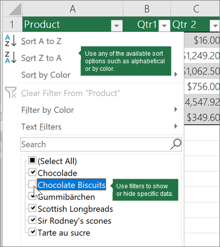
Header row By default, a table has a header row. Every table column has filtering enabled in the header row so that you can filter or sort your table data quickly. For more information, see Filter data or Sort data.

You can turn off the header row in a table. For more information, see Turn Excel table headers on or off.
-
Banded rows Alternate shading or banding in rows helps to better distinguish the data.
-
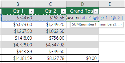
Calculated columns By entering a formula in one cell in a table column, you can create a calculated column in which that formula is instantly applied to all other cells in that table column. For more information, see Use calculated columns in an Excel table.
-
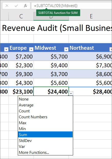
Total row Once you add a total row to a table, Excel gives you an AutoSum drop-down list to select from functions such as SUM, AVERAGE, and so on. When you select one of these options, the table will automatically convert them to a SUBTOTAL function, which will ignore rows that have been hidden with a filter by default. If you want to include hidden rows in your calculations, you can change the SUBTOTAL function arguments.
For more information, also see Total the data in an Excel table.
-
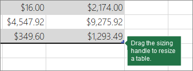
Sizing handle A sizing handle in the lower-right corner of the table allows you to drag the table to the size that you want.
For other ways to resize a table, see Resize a table by adding rows and columns.
Create a table
You can create as many tables as you want in a spreadsheet.
To quickly create a table in Excel, do the following:
-
Select the cell or the range in the data.
-
Select Home > Format as Table.
-
Pick a table style.
-
In the Format as Table dialog box, select the checkbox next to My table as headers if you want the first row of the range to be the header row, and then click OK.
Also watch a video on creating a table in Excel.
Working efficiently with your table data
Excel has some features that enable you to work efficiently with your table data:
-
Using structured references Instead of using cell references, such as A1 and R1C1, you can use structured references that reference table names in a formula. For more information, see Using structured references with Excel tables.
-
Ensuring data integrity You can use the built-in data validation feature in Excel. For example, you may choose to allow only numbers or dates in a column of a table. For more information on how to ensure data integrity, see Apply data validation to cells.
Export an Excel table to a SharePoint site
If you have authoring access to a SharePoint site, you can use it to export an Excel table to a SharePoint list. This way other people can view, edit, and update the table data in the SharePoint list. You can create a one-way connection to the SharePoint list so that you can refresh the table data on the worksheet to incorporate changes that are made to the data in the SharePoint list. For more information, see Export an Excel table to SharePoint.
Need more help?
You can always ask an expert in the Excel Tech Community or get support in the Answers community.
See Also
Format an Excel table
Excel table compatibility issues
Need more help?
Want more options?
Explore subscription benefits, browse training courses, learn how to secure your device, and more.
Communities help you ask and answer questions, give feedback, and hear from experts with rich knowledge.

Webopedia is an online information technology and computer science resource for IT professionals, students, and educators. Webopedia focuses on connecting researchers with IT resources that are most helpful for them. Webopedia resources cover technology definitions, educational guides, and software reviews that are accessible to all researchers regardless of technical background.
Our Brands
-
Terms of Service
-
About
-
Privacy Policy
-
Contact
-
Advertise
-
California – Do Not Sell My Information
Property of TechnologyAdvice.
© 2022 TechnologyAdvice. All Rights Reserved
Advertiser Disclosure: Some of the products that appear on this site are from companies from which TechnologyAdvice receives compensation. This compensation may impact how and where products appear on this site including, for example, the order in which they appear. TechnologyAdvice does not include all companies or all types of products available in the marketplace.
This post discusses ways to retrieve aggregated values from a table based on the column labels.
Overview
Beginning with Excel 2007, we can store data in a table with the Insert > Table Ribbon command icon. If you haven’t yet explored this incredible feature, please check out this CalCPA Magazine article Excel Rules.
Frequently, we need to retrieve values out of data tables for reporting or analysis. This task is fairly easy using traditional lookup functions or conditional summing functions. However, when preparing workbooks to be used on an ongoing basis, we need to keep the formula consistency principle in mind. This means we write consistent formulas within a range, so that we can fill them down and right. Often, this is just a matter of setting the cell references properly, such as relative, absolute, or mixed. However, when our data is stored in a table, we can use structured table references and column headers to build consistent formulas.
Objectives
Let’s identify our goals and objectives before we begin. We have exported some invoice information from our accounting system, and have stored it in a table named tbl_inv, pictured below:
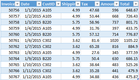
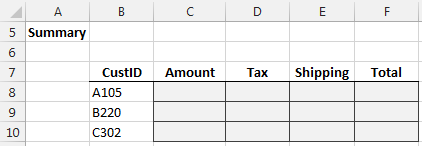
We would like to retrieve values from the table, and aggregate them by customer ID, in order to populate our little summary report, pictured below:
Our first goal is to write a single formula in C8, and then fill it down and to the right. That is, to use consistent formulas.
Next, let’s examine our data and our report. One thing to notice is that each customer may appear on many rows. Thus, we need to use a conditional summing function such as SUMIFS rather than a traditional lookup function, which would only return the related value from the first matching item. If you are not familiar with the SUMIFS function, please check out Multiple Condition Summing in Excel with SUMIFS.
Next, we notice that the report column order differs from the data column order. The report order is custid, amount, tax, shipping, and total. The order of the data columns are custid, shipping, tax, amount, and total. That means we need to write a formula that can accommodate the column order differences.
So, to summarize our objectives:
- Use consistent formulas
- Aggregate multiple rows
- Accommodate column order differences between the data and report
We can meet our objectives by nesting the INDEX and MATCH functions inside of our SUMIFS function to dynamically select the proper sum column. Let’s unpack the formula step by step.
Formula
The first argument of the SUMIFS function is the column of numbers to add. When populating our report’s first column, the column to add is the table’s amount column tbl_inv[Amount]. Our formula would be something like this:
=SUMIFS(tbl_inv[Amount], tbl_inv[CustID],$B8)
However, when populating the next report column, the column of numbers to add is the table’s tax column tbl_inv[Tax]. Our formula would be something like this:
=SUMIFS(tbl_inv[Tax], tbl_inv[CustID],$B8)
Since the first function argument needs to be different for each report column, we are forced to write unique formulas for each column. This does not fall in line with our formula consistency objective. So, the question is, how do we express the first SUMIFS argument so it is dynamic?
One approach is to use the INDEX/MATCH functions. If you are not familiar with the INDEX/MATCH functions, please feel free to check out How to Return a Value Left of VLOOKUP’s Lookup Column for more information. In that blog post, we discussed how the INDEX function returns a cell value, but, it does much more than that.
The INDEX function can actually return a cell value or a range reference. Microsoft describes the function as having two “forms”, the array form and the reference form. It is a fancy way to say that the function can return either a cell value (array form) or a range reference (reference form). We’ll ask the function to return a range reference that can be used as the first SUMIFS argument.
When we are done, the first argument of the SUMIFS function will be dynamic, and it will use INDEX to return a range reference and MATCH to dynamically figure out which column. It will look a little something like this:
=SUMIFS(INDEX(MATCH(...)), tbl_inv[CustID],$B8)
The INDEX/MATCH functions will provide the SUMIFS function with the column of numbers to add. The basic idea is that we will ask the INDEX function to return a reference and we will ask the MATCH function to tell the INDEX function which column to refer to based on the header value. MATCH will look for our report column header, such as Amount, in the table’s header row. The assumption here is that the report header labels match the data header labels.
Since the MATCH function returns the relative position number of a list item, we ask it to tell us the column number of the matching report label. For example, the Amount column is the 6th column, so, it would return 6 to the INDEX function. INDEX uses this information to return the Amount column reference to the SUMIFS function. SUMIFS uses this reference as the column of numbers to add.
Since there are several moving parts, we’ll just ease into this formula. First, let’s replace the first argument of the SUMIFS function with an INDEX function. The resulting formula looks like this:
=SUMIFS(INDEX(tbl_inv,,6), tbl_inv[CustID],$B8)
This formula uses the SUMIFS function to add a column of numbers. The column of numbers to add is the first argument, which is an INDEX function. The first argument of the INDEX function provides the initial range, the whole table, tbl_inv. The second argument of the INDEX function is the row_num argument, and tells the INDEX function which row number to return. Since we want to return all rows, we leave this argument blank. The third argument of the INDEX function is the column_num argument, and we entered 6 because the table’s amount column is the 6th column. Thus, the INDEX function above returns the range reference corresponding to the 6th column in the table to the SUMIFS function.
However, we can’t stop here because we hard-coded the column_num argument 6. If we fill this formula to the right, the 6 would remain and all report column would return the same result, the sum of the amount column. Instead, we need to ask Excel to dynamically figure out which column number the INDEX function should use. And this is accomplished with the MATCH function. The following MATCH function will figure out which column has a matching column header label.
=MATCH(C$7, tbl_inv[#Headers],0)
This function looks for the value in C$7 in the headers row of the table. We use a relative column reference (C) so that it updates as it is filled right, and an absolute row reference ($7) so that it is locked onto the report header row. Note the special structured table reference that refers to the headers row. It starts with the table’s name, tbl_inv, and then #Headers enclosed in square brackets. You can type in this reference or just use your mouse to select it interactively. The third argument, 0, tells the function we are looking for an exact match.
Since the MATCH function above returns 6, we need to nest it inside of the INDEX function. If we nest the MATCH function inside the INDEX function, we get the following:
INDEX(tbl_inv,, MATCH(C$7,tbl_inv[#Headers],0))
This formula segment returns the column reference needed by the SUMIFS function. So, nesting the INDEX/MATCH functions inside the SUMIFS function results in the following:
=SUMIFS(INDEX(tbl_inv,, MATCH(C$7,tbl_inv[#Headers],0)), tbl_inv[CustID],$B8)
We could write this formula in C8, and then fill it down and right to create the report. But, there is one more little detail.
If this workbook is designed to be used on a recurring basis and to remain in place for a long time, then we need to think about ways that a future user could break the workbook and address any risks up front, as discussed in Excel University Volume 1 Chapter 19. We therefore need to consider the different ways that future users may try to fill our formula down and to the right, because the way they fill right could accidentally break our formula.
Specifically, if a user tries to fill the formula right with the fill command, a copy/paste, or, with Ctrl+Enter, then Excel treats the tbl_inv[CustID] reference as absolute. This is good because as we fill the formula right we do want all formulas to reference the customer id column. However, if a user chooses to fill the formula right by dragging the fill handle, then, the reference is treated as relative, meaning, it will also slide to the right and change to tbl_inv[Shipping], tbl_inv[Tax], and so on.
So, to be safe, we’ll modify the reference slightly so that Excel treats it as absolute even if a user fills right with the fill handle. We’ll update it to a single-column range reference: tbl_inv[[CustID]:[CustID]]. The final formula is:
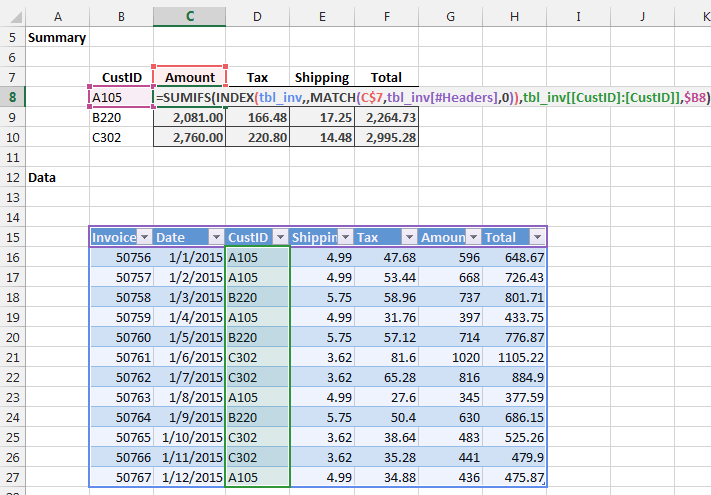
=SUMIFS(INDEX(tbl_inv,,
MATCH(C$7,tbl_inv[#Headers],0)),
tbl_inv[[CustID]:[CustID]], $B8)
We enter the formula in C8, and fill it down and right, and the resulting report is pictured below.
Although it may feel like it took us a long time to get here, the end result is a formula that meets our objectives. It can be filled down and to the right and continue to work, it accommodates column order differences, and it aggregates values.
Conclusion
Generally, it is worth the time to create consistent formulas that can be filled down and right and continue to work for recurring use workbooks because it makes updating them over time faster. Additionally, writing formulas that can accommodate minor structure changes, such as the column orders moving around over time, will help reduce errors and improve efficiency. Although the upfront time investment getting a formula like the one above to work may be significant, you’ll receive your investment back each subsequent period through improved productivity.
Sample File
To check out the Excel file that was used to prepare the screenshots, feel free to download the sample file:
RetrieveTableData
To check up the updated version that replaces the $B8 cell reference with a named reference, feel free to download the sample file:
RetrieveTableData2
Additional Notes
- If you need to retrieve a text string, rather than the sum of numbers, you’ll probably want to use traditional lookup functions, such as VLOOKUP. The workbook sample file includes a VLOOKUP sheet with the relevant formulas.
- If you’d like more assistance with the SUMIFS, INDEX, and MATCH functions, please feel free to check out our online Excel training courses.
- If you have another approach you prefer, please post a comment, we would love to hear about it!
In this post, we’re going to learn everything there is to know about Excel Tables!
Yes, I mean everything and there’s a lot.
This post will tell you about all the awesome features Excel Tables have and why you should start using them.
What is an Excel Table?
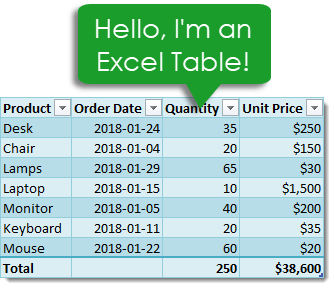
Excel Tables are containers for your data.
Imagine a house without any closets or cupboards to store your things, it would be chaos! Excel tables are like closets and cupboards for your data, they help to contain and organize data in your spreadsheets.
In your house, you might put all your plates into one kitchen cupboard. Similarly, you might put all your customer data into one Excel table.
Tables tell excel that all the data is related. Without a table, the only thing relating the data is proximity to each other.
Ok, so what’s so great about Excel Tables other than being a container to organize data? A lot actually. This post will tell you about all the awesome features tables have and should convince you to start using them.
Video Tutorial
The Parts of a Table
Throughout this post, I’ll be referring to various parts of a table, so it’s probably a good idea that we’re both talking about the same thing.
This is the Column Header Row. It is the first row in a table and contains the column headings that identify each column of data. Column headings must be unique in the table, they cannot be blank and they cannot contain formulas.
This is the Body of the table. The body is where all the data and formulas live.
This is a Row in the table. The body of a table can contain one or more rows and if you try to delete all the rows in a table a single blank row will remain.
This is a Column in the table. A table must contain at least one column.
This is the Total Row of the table. By default, tables don’t include a total row but this feature can be enabled if desired. If it’s enabled, it will be the last row of the table. This row can contain text, formula or remain blank. Each cell in the total row will have a drop down menu that allows selection of various summary formula.
Create a Table from the Ribbon
Creating an Excel Table is really easy. Select any cell inside your data and Excel will guess the range of your data when creating the table. You’ll be able to confirm this range later on. Instead of letting Excel guess the range you can also select the entire range of data in this step.
With the active cell inside your data range, go to the Insert tab in the ribbon and press the Table button found in the Tables section.
The Create Table dialog box will pop up. Excel guesses the range and you can adjust this range if needed using the range selector icon on the right hand side of the Where is the data for your table? input field. You can also adjust this range by manually typing over the range in the input field.
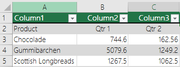
Checking the My table has headers box will tell Excel the first row of data contains the column headers in your table. If this is unchecked Excel will create generic column headers for the table labelled Column 1, Column 2 etc…
Press the Ok button when you’re satisfied with the data range and table headers check box.
Congratulations! You now have an Excel table and your data should look something like the above depending on the default style of your tables.
Contextual Table Tools Design Tab
Whenever you select a cell inside a table, you will notice a new tab appear in the ribbon labelled Table Tools Design. This is a contextual tab and only appears when a table is selected. When the active cell moves outside the table, the tab will disappear again.
This is where all the commands and options related to tables will live. This is where you’ll be able to name your table, find table related tools, enable or disable table elements and change your table’s style.
Create a Table with a Keyboard Shortcut
You can also create a table using a keyboard shortcut. The process is the same as described above but instead of using the Table button in the ribbon you can press Ctrl + T on your keyboard. It’s easy to remember since T is for Table!
There is actually another keyboard shortcut that you can use to create tables, Ctrl + L will also do the same thing. This is a legacy from when tables were called lists (L is for List).
Name a Table
Anytime you create a new table Excel will give it an initial generic name starting with Table1 and increasing sequentially. You should always rename your table with a descriptive and short name.
Not all names are allowed. There are a few rules for a table name.
- Each table must have a unique name within a workbook.
- You can only use letters, numbers and the underscore character in a table name. No spaces or other special characters are allowed.
- A table name must begin with either a letter or an underscore, it can not begin with a number.
- A table name can have a maximum of 255 characters.
Select any cell inside your table and the contextual Table Tools Design tab will appear in the ribbon. Inside this tab you can find the Table Name under the Properties section. Type over the generic name with your new name and press the Enter button when finished to confirm the new name.
Rename a Table
Renaming a table you’ve already named is the same process as naming a table for the first time. If you think about it, when you first name a table you’re actually renaming it from the generic name of Table1 to a new name.
So go back to the Table Tools Design tab and type your new name over the old one in the Table Name and press Enter. Easy, and the name is changed.
Changing your table name this way requires navigating to your table and selecting a cell within it, so it can be tedious if you need to rename a lot of tables across different sheets in your workbook. Instead, you can change any of your table names without going to each table using the Name Manager.
Go to the Formula tab and press the Name Manager button in the Defined Names section. You’ll be able to see all your named objects here. The table objects will have a small table icon to the left of the name. You can filter to show only the table objects using the Filter button in the upper right hand corner and selecting Table Names from the options.
You can then edit any name by selecting the item and pressing the Edit button. You’ll be able to change the name and add some comments to describe the data in your table.
Navigate Tables with the Name Box
You can easily navigate to any table in your workbook using the name box the the left of the formula bar. Click on the small arrow on the right side of the name box and you will see all table names in the workbook listed. Click on any of the tables listed and you will be taken to that table.
Convert a Table Back to a Normal Range
Ok, you changed your mind and don’t want your data inside a table anymore. How do you convert it back into a regular range?
If changing it to a table was the last thing you did, Ctrl + Z to undo your last action is probably the quickest way.
If it wasn’t the last thing you did, then you’re going to need to use the Convert to Range command found in the Table Tools Design tab under the Tools section.
You’ll be prompted to confirm that you really want to convert the table to a normal range. Noooooo, don’t do it, tables are awesome!
If you click on yes, then all the awesome benefits from tables will be gone except for the formatting design. You’ll need to manually clear this from the range if you want to get rid it. You can do this by going to the Home tab then pressing the Clear button found in the Editing section, then selecting Clear Formats.
This can also be done from the right click menu. Right click anywhere in the table and select Table from the menu and then Convert to Range.
Select the Entire Column
If your data is not inside a table then selecting an entire column of the data can be difficult. The usual way would be to select the first cell in the column and then hold Ctrl + Shift then press the Down arrow key. If the column has blank cells, then you might need to press the Down arrow key a few times until you reach the end of the data.
The other option is to select the first cell and then use the scroll bar to scroll to the end of your data then hold the Shift key while you select the last column.
Both options can be tedious if you have a lot of data or there are a lot of blanks cells in the data.
With a table, you can easily select the entire column regardless of blank cells. Hover the mouse cursor over the column heading until it turns into a small arrow pointing down then left click and the entire column will be selected. Left click a second time to include the column heading and any total row in the selection.
Another way to quickly select the entire column is to place the active cell cursor on any cell in the column and press Ctrl + Space. This will select the entire column excluding the column header and total row. Press Ctrl + Space again to include the column headers and total row.
Select the Entire Row
Selecting the entire row is just as easy. Hover the mouse cursor over the left side of the row until it turns into a small arrow pointing left then left click and the entire row will be selected. This works on both the column heading row and total row.
Another way to quickly select the entire row is to place the active cell cursor on any cell in the row and press Shift + Space.
Select the Entire Table
It’s also possible to select the entire table and there are a couple different ways to do this.
You can place the active cell cursor inside the table and press Ctrl + A. This will select the entire body of the table excluding the column headers and total row. Press Ctrl + A again to include the column headers and total row.
Hover the mouse over the top left hand corner of the table until the cursor turns into a small black diagonal right and downward pointing arrow. Left click once to select only the body. Left click a second time to include the header row and total row.
You can also select the table with the mouse. Place the active cell inside the table and then hover the mouse cursor over any edge of the table until it turns into a four way directional arrow then left click. This will also select the column headers and total row.
Select Parts of the Table from the Right Click Menu
You can also select rows, columns or the entire table using the right click menu. Right click anywhere on the row or column you want to select then choose Select and pick from the three options available.
Add a Total Row
You can add a total row which allows you to display summary calculations in the last row of your table.
Adding summary calculations at the bottom of your data can be dangerous as they might end up getting included by accident in a pivot table using the data. This is another advantage of tables, as the total row won’t be included in any pivot tables created with the table.
To enable the total row, go to the Table Tools Design tab and check the Total Row box found in the Table Style Options section.
You can temporarily disable the total row without losing the formulas you added to it. Excel will remember the formulas you had and they will appear when you enable it again.
Each cell in the total row has a drop down menu that allows you to pick various aggregating functions to summarize the column of data above.
You can also enter your own formulas. I’ve entered a SUMPRODUCT formula in the Unit Price total to sum the Quantity x Unit Price to calculate a total sale amount. Formulas don’t have to return a number, they can also be text results.
Constant numerical or text values are also allowed anywhere in the total row. In fact the leftmost column will usually contain the text Total by default.
Add a Total Row with a Right Click
You can also add the total row with a right click. Right click anywhere on the table and the choose Table and Total Row from the menu.
Add a Total Row with a Keyboard Shortcut
Another way to quickly add the total row is to place the active cell cursor inside your table and use the Ctrl + Shift + T keyboard shortcut.
Disable the Column Header Row
The column header row is enabled by default, but you can disable it. This doesn’t delete the column headers, it’s essentially like hiding them as you will still reference columns based on the column header name.
Go to the Table Tools Design tab and uncheck the Total Row box found in the Table Style Options section.
Add Bold Format to the First or Last Columns
You can enable a bold formatting on either your first or last column to highlight it and draw attention to them over other columns.
Go to the Table Tools Design tab and check either of the First Column or Last Column boxes (or both) found in the Table Style Options section.
Add Banded Rows or Columns
Banded rows are already enabled by default, but you can turn them off if you want. Banded columns are disabled by default, so you need to enable them if you want them.
To enable or disable either, go to the Table Tools Design tab and check or uncheck the Banded Rows or Banded Columns boxes found in the Table Style Options section.
I generally find banded rows are the most useful and if you enable banded columns at the same time, the table starts to look a little messy. I recommend one or the other and not both at the same time.
- Table with no banded rows or columns.
- Table with banded rows only.
- Table with banded columns only.
- Table with both banded rows and columns.
Table Filters
By default, the table filters option is enabled. You can disable them from the Table Tools Design tab by unchecking the Filter Button box found in the Table Style Options section.
You can also toggle the filters on or off from the active table by using the regular filter keyboard shortcut of Ctrl + Shift + L.
If you left click on any of the filters, it will bring up the familiar filter menu where you can sort your table and apply various filters depending on the type of data in the column.
The great thing about table filters is you can have them on multiple tables in the same sheet simultaneously. You will need to be careful though as filtered items in one table will affect the other tables if they share common rows. You can only have one set of filters at a time in a sheet of data without tables.
Total Row with Filters Applied
When you select a summary function from the drop down menu in the total row, Excel will create the corresponding SUBTOTAL formula. This SUBTOTAL formula ignores hidden and filtered items. So when you filter your table these summaries will update accordingly to exclude the filtered values.
Note that the SUMPRODUCT formula in the Unit Price column still includes all the filtered values while the SUBTOTAL sum formula in the Quantity column does not.
Column Headers Remain Visible When Scrolling
If you scroll down while the active cell is in a table, its column headers will remain visible along with the filter buttons. The table’s column headings will get promoted into the sheet’s column headings where we would normally see the alphabetic column name.
This is extremely handy when dealing with long tables as you won’t need to scroll back up to the top to see the column name or use the filters.
Automatically Include New Rows and Columns
If you type or copy and paste new data into the cells directly below a table, they will automatically be absorbed into the table.
The same thing happens when you type or copy and paste into the cells directly to the right of a table.
Automatically Fill Formulas Down the Entire Column
When you enter a formula inside a table it will automatically fill the formula down the entire column.
Even when a formula has already been entered and you add new data to the row directly below the table any existing formulas will automatically fill.
Editing an existing formula in any of the cells will also update the formula in the entire column. You’ll never forget to copy and paste down a formula again!
Turn Off the Auto Include and Auto Fill Settings
You can turn off the feature that automatically adds new rows or columns and fills down formulas.
Go to the File tab and select Options. Choose Proofing then press the AutoCorrect Options button. Navigate to the AutoFormat As You Type tab in the AutoCorrect dialog box.
Unchecking the Include new rows and columns in table option allows you to type directly underneath or to the right of a table without it absorbing the cells.
Unchecking the Fill formulas in tables to create calculated columns option means the formulas in a table will no longer automatically fill down the column.
Resize with the Handle
Every table comes with a Size Handle found in the bottom rightmost cell of the table.
When you hover the mouse over the handle, the cursor will turn into a double-sided diagonally slanting arrow and you can then click and drag to resize the table. You can either expand or contract the size. Data will be absorbed into the table or removed from it accordingly.
Resize with the Ribbon
You can also resize the table from the ribbon. Go to the Table Tools Design tab and press the Resize Table command in the Properties section.
The Resize Table dialog box will pop up and you’ll be able to select a new range for your table. Use the range selector icon to select a new range. You can select either a larger or smaller range, but The table headers will need to remain in the same row and the new table range must overlap the old table range.
Add a New Row with the Tab Key
You can add a new blank row to a table with the Tab key. Place the active cell cursor inside the table on the cell containing the sizing handle and press the Tab key.
The tab key act like a carriage return and the active cell is taken to the rightmost cell on a new line that’s added directly below.
This is a handy shortcut to know because when the total row is enabled, it’s not possible to add a new row by typing or copying and pasting data directly below the table.
Insert Rows or Columns
You can insert extra rows or columns into a table with a right click. Select a range in the table and right click then choose Insert from the menu. You can then either choose to insert Table Columns to the Left or Table Rows Above.
Table Columns to the Left will insert the number of columns selected to the left of the selection and the number of rows in the selection is ignored.
Table Rows Above will insert the number of rows selected just above the selection and the number of columns in the selection is ignored.
Delete Rows or Columns
Deleting rows or columns has a similar story to inserting them. Select a range in the table and right click then choose Delete from the menu. You can then either choose to delete Table Columns or Table Rows.
Formats in a Table Automatically Apply to New Rows
When you add new data to your table, you don’t need to worry about applying formatting to match the rest of the data above. Formatting will automatically fill down from above if the formatting has been applied to the entire column.
I’m not just talking about the table style formats. Other formatting like dates, numbers, fonts, alignments, borders, conditional formatting, cell colours etc. will all automatically fill down if they’ve been applied to the whole column.
If you’ve formatted all your numbers as a currency in a column and you add new data, it too will get the currency format applied to it.
You never need to worry about inconsistent formatting in your data.
Add a Slicer
You can add a slicer (or several) to a table for an easy to use filter and visual way to see what items the table is filtered on.
Go to the Table Tools Design tab and press the Insert Slicer button found in the Tools section.
Change the Style
Changing the styling of a table is quick and easy. Go to the Table Tools Design select a new style from the selection found in the Table Styles section. If you left click the small downward arrow on the right hand side of the styles palette, it will expand to show all available options.
These table styles apply to the whole table and will also apply to any new rows or columns added later on.
There are many options to choose from including light, medium and dark themes. As you hover over the various selections, you’ll be able to see a live preview in the worksheet. The style won’t actually change until you click on one though.
You can even create your own New Table Style.
Set a Default Table Style
You can set any of the styles available as the default so that when you create a new table you don’t need to change the style. Right click on the style you want to set as the default and then choose Set As Default from the menu.
Unfortunately, this is a workbook level setting and will only affect the current workbook. You will need to set the default for each workbook you create if you don’t want the application default option.
Only Print the Selected Table
When you place the active cell cursor inside a table and then try to print, there is an option to only print the selected table. Go to the Print menu screen by either going to the File tab and selecting Print or using the Ctrl + P keyboard shortcut, then select Print Selected Table in the settings.
This will remove any items from the print area that are not in the table.
Structured Referencing
Tables come with a useful feature called structured referencing which helps to make range references more readable. Ranges within a table can be referred to using a combination of the table name and column headings.
Instead of seeing a formula like this =SUM(D3:D9) you might see something like this =SUM(Sales[Quantity]) which is much easier to understand the meaning of.
This is why naming your table with a short descriptive name and column headings is important as it will improve the readability of the structured references!
When you reference specific parts of a table, Excel will create the reference for you so you don’t need to memorize the reference structure but it will help to understand it a bit.
Structured references can contain up to three parts.
- This is the table name. When referencing a range from inside the table this part of the reference is not required.
- These are range identifiers and identify certain parts of the reference for a table like the headers or total row.
- These are the column names and will either be a single column or a range of columns separated by a full colon.
Example of structured References for a Row
=Sales[@[Unit Price]]will reference a single cell in the body.=Sales[@[Product]:[Unit Price]]will reference part of the row from the Product column to the Unit Price column including all columns in between.=Sales[@]will reference the full row.
Example of Structured References for Columns
=Sales[Unit Price]will reference a single column and only include the body.=Sales[[#Headers],[#Data],[Unit Price]]will reference a single column and include the column header and body.=Sales[[#Data],[#Totals],[Unit Price]]will reference a single column and include the body and total row.=Sales[[#All],[Unit Price]]will reference a single column and include the column header, body and total row.
Example of Structured References for the Total Row
=Sales[#Totals]will reference the entire total row.=Sales[[#Totals],[Unit Price]]will reference a cell in the total row.=Sales[[#Totals],[Product]:[Unit Price]]will reference part of the total row from the Product column to the Unit Price column including all columns in between.
Example of Structured References for the Column Header Row
=Sales[#Headers]will reference the entire column header row.=Sales[[#Headers],[Order Date]]will reference a cell in the column header row.=Sales[[#Headers],[Product]:[Unit Price]]will reference part of the column header row from the Product column to the Unit Price column including all columns in between.
Example of Structured References for the Table Body
=Saleswill reference the entire body.=Sales[[#Headers],[#Data]]will reference the entire column header row and body.=Sales[[#Data],[#Totals]]will reference the entire body and total row.=Sales[#All]will reference the entire column header row, body and total row.
Using Intellisense
One of the great things about a table is the structured references will appear in Intellisense menus when writing formulas. This means you can easily write a formula using the structured references without remembering all the fields in your table.
After typing the first letter of the table name, the IntelliSense menu will show the table name among all the other objects starting with that letter. You can use the arrow keys to navigate to it and then press the Tab key to autocomplete the table name in your formula.
If you want to reference a part of the table, you can then type a [ to bring up all the available items in the table. Again, you can navigate with the arrow keys and then use the Tab key to autocomplete the field name. Then you can close the item with a ].
Turn Off Structured Referencing
If you’re not a fan of being forced to use the structured referencing system, then you can turn it off. Any formulas that have been entered using the structured referencing will remain and they will still work the same. You’ll also still be able to use structured references, Excel just won’t automatically create them for you.
To turn it off, go to the File tab and then select Options. Choose Formulas on the side pane and then uncheck the Use table names in formulas box and press the Ok button.
Summarize with a PivotTable
You can create a pivot table from your table in Table Tools Design tab, press the Summarize with PivotTable button found in the Tools section. This will bring up the Create PivotTable window and you can create a pivot table as usual.
This is the same as creating a pivot table from the Insert tab and doesn’t give any extra options specific to tables.
Remove Duplicates from a Table
You can create remove duplicate rows of data from your table in Table Tools Design tab, press the Remove Duplicates button found in the Tools section. This will bring up the Remove Duplicates window and delete duplicate values for one or more columns in the table.
This is the same as removing duplicates from the Data tab and doesn’t give any extra options specific to tables.
About the Author
John is a Microsoft MVP and qualified actuary with over 15 years of experience. He has worked in a variety of industries, including insurance, ad tech, and most recently Power Platform consulting. He is a keen problem solver and has a passion for using technology to make businesses more efficient.