What is choose function in excel

Excel CHOOSE Function – How To Use

The CHOOSE function in MS Excel returns a value from a list of values based on an index number. The list of values can also be specified as cell references. Choose function can support up to 254 values.

Although on its own CHOOSE function may not look much valuable, but when combined with other functions, it can work wonders. The function has served as a handy fallback option since its introduction to Office in 2003.

In this tutorial, we are going to see the basics of the excel CHOOSE function, and then gradually, we will progress on to more complicated scenarios.

Table of Contents

Syntax

The syntax of the CHOOSE function is as follows:

Arguments:

index_num – The index number or the position of a value in the list that is to be displayed.
value1 – The first value in the list.
value2 – The second value in the list. Entering this argument is optional.

Important Characteristics of CHOOSE Function in Excel

• CHOOSE function can only support up to 254 values, this implies that the ‘index_num’ specified in the function must be a number between 1 and 254.
• If ‘index_num’ is an array, the array as a whole is processed as opposed to finding a match value by value.
• If the ‘index num’ in the function is out of this range i.e., less than 1 or greater than the number of values, the function returns a #VALUE! error.
• If the ‘value’ arguments are not enclosed in quotation marks, the function returns a #NAME? error.
• If the ‘index_num’ is a fraction, it will be rounded to the lowest integer eg., 2¾ will be rounded down to 2 instead of 3.
• The arguments can be numbers, cell references, defined names, formulas, functions, or text.

Examples of CHOOSE Function

Let’s have a look at a simple example of the CHOOSE function before going into more complex scenarios.

Example 1 – Plain Vanilla Version of CHOOSE Function

In this case, we will pass a list of 3 countries to the CHOOSE function as values, and then analyze the result by changing the ‘index_num’ argument.

So, our first formula would be:

In the above formula, since the ‘index_num’ parameter is set to 1 so the formula returns the first country (i.e. United States) out of the supplied list of values.

Similarly, by changing the ‘index_num’ parameter in the following formulas we can get different results:

Example 2 – CHOOSE Function with SUM Function

In this example, we will try to see how to perform selective summation in excel by using the SUM and CHOOSE functions together. The good old, and most basic, SUM function needs no introduction and it does plainly as said; totals a series of numbers.

Now we will take you through selective summation.

Here, we have data from 3 classes each class is further divided into sections. Each section has 20 to 25 students. Our objective is to calculate the total number of students in any one of the given class (say class 9th).

In order to do this, we can use the CHOOSE and SUM functions as follows:

Now let’s dissect this formula –

In the above formula, the CHOOSE function is supplied with cell ranges – B2:B5,C2:C5,D2:D5

• Cells «B2:B5» have the count of students of sections A, B, C, and D of Class 8.
• Cells «C2:C5» have the count of students of sections A, B, C, and D of Class 9.
• Cells «D2:D5» have the count of sections A, B, C, and D of Class 10.

Next, the ‘index_num’ parameter is set to 2, which points to the range C2:C5. This means that the result of the CHOOSE function in our case would be C2:C5. This cell range is passed to the SUM function and it performs a summation on the numbers present in the given range and returns the final result.

To bring up the total of a different class, we only have to change the ‘index_num’ in the formula. If the ‘index_num’ parameter is set to 1, the CHOOSE function would return the range B2:B5 (i.e. Class 8th). Similarly, when the ‘index_num’ parameter is set to 3, the CHOOSE function would return the range D2:D5 (i.e. Class 10th)

Example 3 – CHOOSE as an Alternative to Nested IF Statements

We all know, the role of an IF function is to return a value based on the stated condition. IF functions can be nested within each other to develop formulas for handling complex logic.

Functionally CHOOSE function is very similar to nested IF statements. However, CHOOSE makes it super easy to combine multiple conditions into one formula instead of having multiple IF functions nested within one another.

Let’s try to understand this with an example.

Here we have a list of students along with their scores. Based on the scores we have to populate their ratings against their names.

Scores less than 70 are rated «Poor», scores between 71 to 80 are rated as «Average», scores between 81 to 90 are rated as «Good» and a score of 91 or more is rated as «Excellent».

We can have a CHOOSE function to do this:

Let’s try to understand how this formula works –

On analyzing the formula, we can see the only thing that looks different here is the ‘index_num’ parameter.

Here instead of a usual numeric value, we have an expression : (B2>=0) + (B2>=71) + (B2>=81) + (B2>=91)

Actually, this expression is being evaluated to a numeric value, let’s understand how.

B2 cell has a value of 77. So, the expression becomes : (77>=0) + (77>=71) + (77>=81) + (77>=91)

Evaluating each condition inside the expression:

• The condition 77 is greater than equal to 0 is TRUE.
• The condition 77 is greater than equal to 71 is TRUE.
• The condition 77 is greater than equal to 81 is FALSE.
• The condition 77 is greater than equal to 1 is FALSE.

So, the expression becomes : TRUE + TRUE + FALSE + FALSE

Since, Excel treats TRUE as 1 and FALSE as 0 so the expression can further be simplified to : 1 + 1 + 0 + 0 . Which is equal to 2, hence in the first case index_num is considered as 2.

And «Average» is the value that corresponds to index 2 and hence is displayed as the result.

If the same logic was to be written using the nested IF functions, the formula would have been:

As you can see, there is 1 IF statement for each rating which means four IF statements in this case. We definitely know which function we prefer here.

Example 4 – CHOOSE Function to Generate Random Data

By now we are well familiar with the CHOOSE function’s ability to compute data. Did you know you can generate random data in Excel, with CHOOSE function?

To do this we can make use of CHOOSE function and the RANDBETWEEN function.

The RANDBETWEEN (random between) function in Excel returns an integer randomly from the specified range of numbers.

In order to generate random data you need to use the CHOOSE and RANDBETWEEN functions together, let’s see this with an example:

Beginning the first semester of preschool, all students are to be assigned to one of 4 houses (Gryffindor, Hufflepuff, Ravenclaw, and Slytherin). Yes, I am a Harry Potter fan 🙂

Our objective is to randomly assign students a house in excel.

For this, we can make use of the formula –

In the formula, the houses are assigned numbers 1 – 4. Gryffindor corresponds to 1, Hufflepuff corresponds to 2, Ravenclaw corresponds to 3 while Slytherin corresponds to 4.

The RANDBETWEEN function generates a random number (from 1 to 4) for student Riley (in this case, the number was «1»). Next, the CHOOSE function picks the relevant «value» argument and returns the result in the form of a house name (Gryffindor).

This is how the rest of column B is populated; the formula assigns a house to each student in line with the number randomly generated.

Example 5 – CHOOSE to Get Day Name from a Date

The CHOOSE function can also be used to get day names (i.e. Monday, Tuesday, etc.) from a date.

I agree that there are multiple ways to do this, for instance, you can make use of the TEXT function and retrieve this very easily like –

Although these formulas give you the desired result but do not allow you to have control over the result, for example instead of ‘Saturday’ you only want to show ‘Sa’. For all such scenarios, CHOOSE function can be quite handy.

The formula would be –

In the above formula, the WEEKDAY function computes the given date and returns a number (1-7) corresponding to the day of the week. With default settings, Sunday corresponds to 1 and Saturday to 7. This number is then passed to the CHOOSE function as ‘index_num’ and the CHOOSE function picks and returns the value corresponding to the ‘index_num’

Example 6 – CHOOSE to Get Month Name from a Date

Just like the day name example above, the month name (January, February, etc.) can also be derived from a date with the help of CHOOSE function. Similar arguments hold true for converting date to month.

To do this we can make use of the following formula –

In the above formula, we have used the CHOOSE function along with the MONTH function. The MONTH function accepts a date and returns a number from (1 – 12) corresponding to the month of the year. With default settings, January corresponds to 1 and December to 12. This number is then passed to the CHOOSE function as ‘index_num’ and the CHOOSE function picks and returns the value corresponding to the ‘index_num’.

Example 7 – CHOOSE for Left VLOOKUP

We all are aware of the VLOOKUP function, it searches a vertically arranged table meaning the data must be in columnar form.

A huge limitation of the VLOOKUP function is that it only works rightward. This means that the lookup column must be the left-most column in your data set. This restriction can be bypassed with the help of the CHOOSE function which can perform the search leftward.

Let’s understand this with an example:

We have a dataset with ‘Student Names’ and their ‘Scores’. Our objective is to find the score of a particular student named «Rolando».

To make a simple VLOOKUP work, we would have to arrange the table with the «Student Name» column first and the «Score» column second because the function only works rightward.

However, by making use of the CHOOSE function along with the VLOOKUP we can get this working. Following is the formula –

Let’s try to understand the above formula by breaking it into two parts – the inner CHOOSE function and the outer VLOOKUP function.

First, let’s talk about the CHOOSE function because this is where most of the heavy weight lifting is being done. Till now we have only seen the examples of the CHOOSE function with a single index number as the first argument but here we are making use of an array constant containing two numbers <1,2>.

This is essentially equivalent to asking the CHOOSE function to return two values instead of 1. The next important part of the function is the sequence of ranges provided in the values parameter i.e. B2:B11, A2:A11. Notice that how cleverly we are providing the ranges in the revered order.

These two things enable the CHOOSE function to return an array with two columns where the first column corresponds to the «Student Names» while the second one corresponds to their «Scores» (i.e. swapping the original column positions)

Now let’s talk about the second part – the VLOOKUP function. The VLOOKUP function is pretty straightforward, it searches for the value at D6 in the range provided by the CHOOSE function (the range formed by swapping the column positions), requests for the values in the 2nd column of the given range with an exact match.

And we get the expected result. Hurray!

That’ll be all from the CHOOSE function. Here’s hope we gave you a good idea on how to choose with the CHOOSE. We’ll be coming right back with another Excel-lent function soon. Ciao!

Subscribe and be a part of our 15,000+ member family!

Now subscribe to Excel Trick and get a free copy of our ebook «200+ Excel Shortcuts» (printable format) to catapult your productivity.

Источник

CHOOSE function

This article describes the formula syntax and usage of the CHOOSE function in Microsoft Excel.

Description

Uses index_num to return a value from the list of value arguments. Use CHOOSE to select one of up to 254 values based on the index number. For example, if value1 through value7 are the days of the week, CHOOSE returns one of the days when a number between 1 and 7 is used as index_num.

Syntax

CHOOSE(index_num, value1, [value2], . )

The CHOOSE function syntax has the following arguments:

Index_num Required. Specifies which value argument is selected. Index_num must be a number between 1 and 254, or a formula or reference to a cell containing a number between 1 and 254.

If index_num is 1, CHOOSE returns value1; if it is 2, CHOOSE returns value2; and so on.

If index_num is less than 1 or greater than the number of the last value in the list, CHOOSE returns the #VALUE! error value.

If index_num is a fraction, it is truncated to the lowest integer before being used.

Value1, value2, . Value 1 is required, subsequent values are optional. 1 to 254 value arguments from which CHOOSE selects a value or an action to perform based on index_num. The arguments can be numbers, cell references, defined names, formulas, functions, or text.

If index_num is an array, every value is evaluated when CHOOSE is evaluated.

The value arguments to CHOOSE can be range references as well as single values.

For example, the formula:

which then returns a value based on the values in the range B1:B10.

The CHOOSE function is evaluated first, returning the reference B1:B10. The SUM function is then evaluated using B1:B10, the result of the CHOOSE function, as its argument.

Examples

Copy the example data in the following table, and paste it in cell A1 of a new Excel worksheet. For formulas to show results, select them, press F2, and then press Enter. If you need to, you can adjust the column widths to see all the data.

Источник

The CHOOSE Function in Excel returns a value from the given data range (array) when the position (index) is specified by the user. This lookup and reference function of excel is most commonly used to create scenarios in financial models.

Syntax

The syntax of the CHOOSE function is stated as follows:

The CHOOSE function accepts the following arguments:

#1 – Index_num: This is the position of the value to choose from. It is a number between 1 and 254. It can also be a cell referenceCell reference in excel is referring the other cells to a cell to use its values or properties. For instance, if we have data in cell A2 and want to use that in cell A1, use =A2 in cell A1, and this will copy the A2 value in A1.read more or a function giving a numerical value. It can be in any of the following forms:

• 5
• B2
• “=RANDBETWEEN(2,8)”

Note: If “index_num” is entered as a fraction, it is truncated to the lowest integer at the time of use.

#2 – Value1, [value2], [value3]: This is the data list from which a value is to be returned. It can be a set of numbers, cell referencesCell reference in excel is referring the other cells to a cell to use its values or properties. For instance, if we have data in cell A2 and want to use that in cell A1, use =A2 in cell A1, and this will copy the A2 value in A1.read more, cell references as arrays, text, formulas, or functions. It can be in any of the following forms:

• 1, 2, 3, 4, 5
• Sunday, Monday, Tuesday
• A5, A7, A9
• A2:A7, B2:B7, C2:C7, D2:D7

The “index_num” and “value1” are mandatory arguments. The rest of the arguments are optional.

How to Use CHOOSE Function in Excel? (With Examples)

Let us consider the following examples.

You can download this CHOOSE Function Excel Template here – CHOOSE Function Excel Template

Example #1

We have 6 data points, namely–2, 3, 10, 24, 8, and 11. We want to choose the 4^th element.

We apply the formula “=CHOOSE(4,2,3,10,24,8,11)” or “=CHOOSE(4,A3,A4,A5,A6,A7,A8).”

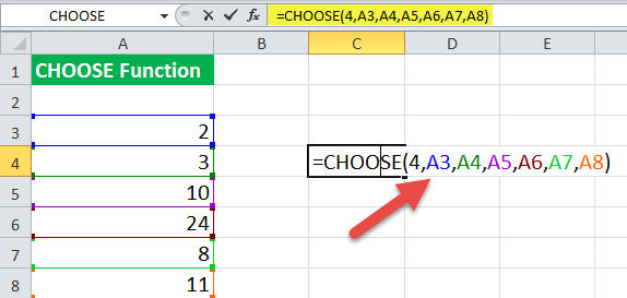
It returns the output 24. If A4 is selected as the index value, it returns 10. This is because A4 corresponds to 3. The third value in the dataset is A5, i.e., 10.

Example #2

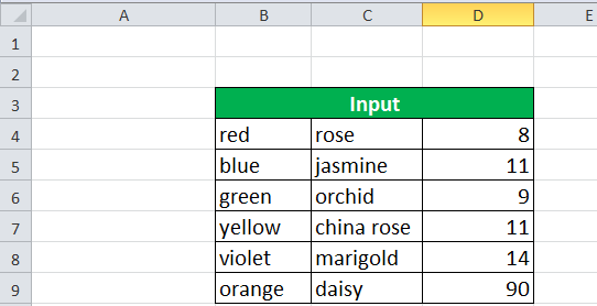
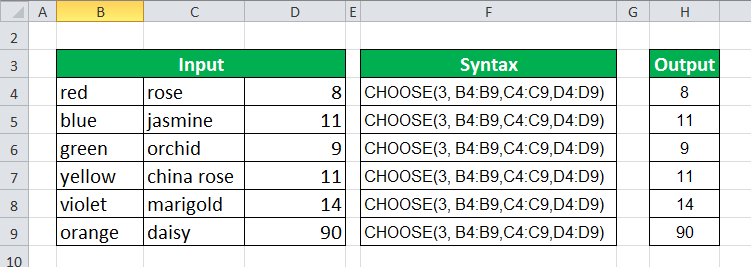
We have three columns containing a list of colors, flowers, and numbers. We want to choose a value from the array of values. We want to choose the third value.

We apply the following CHOOSE formula in Excel.

“=CHOOSE(3,B4:B9,C4:C9,D4:D9)”

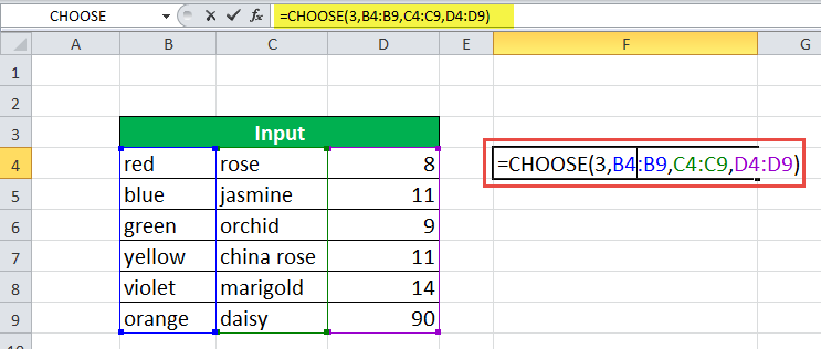
The third value is a list of values “D4:D9,” which is greater than or equal to the input values of column D (8,11,9,11,14,90). So, the output of the formula is the same as the list of values of “D4:D9.”

In a single cell, the formula returns only a single value as an output from the list. This selection is not random and depends on the position of the cell in which the answer is required.

In cell F4, the formula “=CHOOSE(3, B4:B9,C4:C9,D4:D9)” gives the output 8, which corresponds to the value in cell D4.

Similarly, in cell F5, the same input gives 11, which corresponds to the value in cell D5.

Example #3

Let us add one more column to our input of the previous example. We apply the following formula to choose the fourth value.

“=CHOOSE(4,A3:A8,B3:B8,C3:C8,D3:D8)”

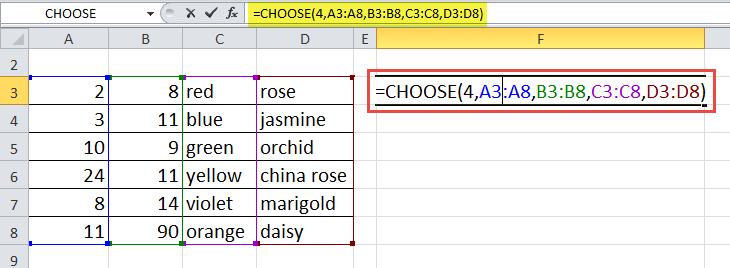
The output is shown in the succeeding image.

Example #4

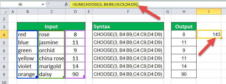
The CHOOSE function can be combined with other functions like the sum, average, mean, etc. Working on the data given in the previous example, we want a sum of “D4:D9.”

We apply the formula “=SUM(CHOOSE(3, B4:B9,C4:C9,D4:D9)).” It gives the sum of the third set of values corresponding to “D4:D9.”

The formula returns the output 143, as shown in the succeeding image.

CHOOSE Function for Random Data

At times, a random grouping of data is required, like in clinical studies, machine learning, and so on. The CHOOSE function can be used to group data randomly. The following example explains how to group data into different classes randomly.

Example #5

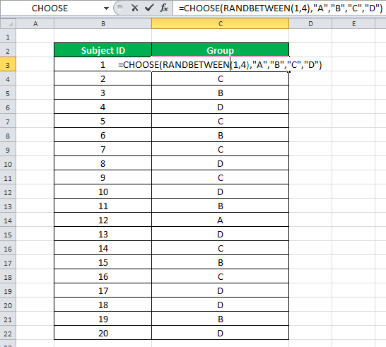
We have a list of 20 subject IDs. We want to group this data into classes–A, B, C, and D.

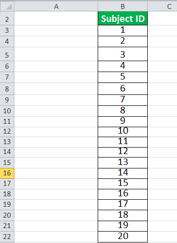
We apply the following formula for selecting the groups A, B, C, and D randomly. “=CHOOSE(RANDBETWEEN(1,4),”A”,”B”,”C”,”D”).”

The function “=RANDBETWEEN(1,4)” selects a random value between 1 to 4. This function is used here as an index value. So, the index value will be randomized from 1 to 4. This means if the index value is 1, it returns A. If the index value is 2, it returns B, and so on.

In this way, the data can be classified into any number of classes with the help of the RANDBETWEEN function of ExcelRANDBETWEEN excel formula determine random numbers between two extreme variables (bottom and top numbers). The user needs to fill in the bottom and top numbers in the syntax =RANDBETWEEN (bottom, top) to acquire the random integer.read more.

CHOOSE Function for Selecting Month

The CHOOSE function can be used to select a day or month from the given data. The following example explains how to extract and return the month from a date.

Example #6

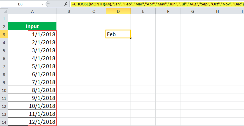
We have a list of dates in column A. The input values in “A3:A14” are shown in the succeeding image. We want to extract the month for the second date value (A4).

We apply the following formula.

“=CHOOSE(MONTH(A4),”Jan”,”Feb”,”Mar”,”Apr”,”May”,”Jun”,”Jul”,”Aug”,”Sep”,”Oct”,”Nov”,”Dec”)”

The formula returns “Feb,” as shown in the succeeding image.

CHOOSE Function With VLOOKUP

The CHOOSE function can be linked with the VLOOKUP function The VLOOKUP excel function searches for a particular value and returns a corresponding match based on a unique identifier. A unique identifier is uniquely associated with all the records of the database. For instance, employee ID, student roll number, customer contact number, seller email address, etc., are unique identifiers.
read moreto obtain the desired value.

Example #7

We have a list of student IDs (B6:B12), student names (C6:C12), and marks (D6:D12) as shown in the following image.

We apply the following formula to find the student’s name with the help of the corresponding ID.

“=VLOOKUP(ID,CHOOSE({1,2},B6:B12,C6:C12),2,0)”

Say we want the name corresponding to the ID in cell F6. So, we replace this ID with the cell reference, as shown in the following image.

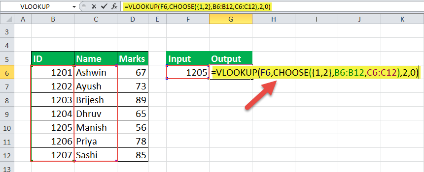
The formula returns the output “Manish.”

Similarly, the marks of a student can be retrieved with the help of the ID or the name. For this, we replace “C6:C12” with “D6:D12.” This returns the output 56.

Example #8

We have three cases with different growth percentages. The principal amount is $100,000. The current amount is “principal amount+(principal amount*growth).” We want the current amount for case 1.

We apply the following formula in Excel.

“=E6+(E6*VLOOKUP(B11,CHOOSE({1,2},A6:A8,B6:B8),2,0))”

This formula is a slight extension of the formula used in Example #7.

The formula returns the amount of $102,000 for case 1.

The Errors in the Usage of CHOOSE Function

1. It returns “#VALUE! error#VALUE! Error in Excel represents that the reference cell the user has either entered an incorrect formula or used a wrong data type (mostly numerical data). Sometimes, it is difficult to identify the kind of mistake behind this error.read more” if:

• the “index_num” argument is greater than the number of values to choose from
• the “index_num” argument does not correspond to a numeric value

1. It returns “#NAME? error” if:

• the value arguments are supplied as text arguments without quotes
• valid cell references are not provided as arguments

Frequently Asked Questions

Recommended Articles

This has been a guide to CHOOSE Function in Excel. Here we discuss the CHOOSE Excel Formula and how to use it along with practical examples and downloadable Excel templates. You can have a look at other articles on Excel functions –

• Excel Convert FunctionAs the word itself, the Excel CONVERT function defines that it can convert the numbers from one measurement system to another measurement system.read more
• Excel Mathematical FunctionMathematical functions in excel refer to the different expressions used to apply various forms of calculation. The seven frequently used mathematical functions in MS excel are SUM, AVERAGE, AVERAGEIF, COUNTA, COUNTIF, MOD, and ROUND.read more
• Max Formula in ExcelThe MAX Formula in Excel is used to calculate the maximum value from a set of data/array. It counts numbers but ignores empty cells, text, the logical values TRUE and FALSE, and text values.read more
• Find Errors in ExcelTo check for errors in a worksheet, go to the home tab> find & select option> go to special and then option> formulas and enable errors.read more