
A cell range in an Excel file is a collection of selected cells.A cell range can be referred to in a formula as well. In a spreadsheet, a cell range is defined by the reference of the upper left cell (minimum value) of the range and the reference of the lower right cell (maximum value) of the range.
Contents
- 1 What is cell range explain with example?
- 2 How do you find the range of cells in Excel?
- 3 What are cells and ranges of cells?
- 4 What is cell range?
- 5 What do you mean by range?
- 6 How do you find the range?
- 7 How do you use range in Excel?
- 8 What is difference between cell and cell range in excel?
- 9 What is range in spreadsheet?
- 10 What is difference between cell and range in excel?
- 11 What is cell range Class 9?
- 12 Why is it called range?
- 13 What does range mean in a passage?
- 14 Where is the range in a function?
- 15 What are the uses of range?
- 16 How do you find range of a function?
- 17 What is range explain with formula?
- 18 What is column range?
- 19 What is the difference between cell address and cell range?
- 20 Which of the following is an example of cell range?
What is cell range explain with example?
When referring to a spreadsheet, the range or cell range is a group of cells within a row or column. For example, in the formula =sum(A1:A10), the cells in column A1 through A10 are the range of cells that are added together.For example, in the formula =sum(A1+B2+C3), the cells A1, B2, and C3 are added together.
How do you find the range of cells in Excel?
Then, hold down CTRL while you click the names of other cells or ranges in the Name box. To select an unnamed cell reference or range, type the cell reference of the cell or range of cells that you want to select, and then press ENTER. For example, type B3 to select that cell, or type B1:B3 to select a range of cells.
What are cells and ranges of cells?
The location of a cell on a worksheet is given by its column letter and its row number (e.g. “A1”). This is often referred to as the Cell Address. All the cells on a worksheet are separated by grey lines, known as gridlines and a group of adjacent cells is known as a Range of cells.
A cell range in an Excel file is a collection of selected cells.In a spreadsheet, a cell range is defined by the reference of the upper left cell (minimum value) of the range and the reference of the lower right cell (maximum value) of the range.
What do you mean by range?
The difference between the lowest and highest values. In {4, 6, 9, 3, 7} the lowest value is 3, and the highest is 9, so the range is 9 − 3 = 6. Range can also mean all the output values of a function.
How do you find the range?
The range is the difference between the biggest and the smallest number.
- To find the range, subtract the lowest number from the biggest number.
- Eg 100 – 3 = 97.
- The range is 97.
How do you use range in Excel?
Another way to make a named range in Excel is this:
- Select the cell(s).
- On the Formulas tab, in the Define Names group, click the Define Name button.
- In the New Name dialog box, specify three things: In the Name box, type the range name.
- Click OK to save the changes and close the dialog box.
What is difference between cell and cell range in excel?
A cell is a single box in the excel spreadsheet which has only one row and one column address. In Excel, the rows are listed as numbers and the columns are named as letters.Cell is a unit and cell range refers to more than one cell. In other words cell is singular while cell range is plural. Hope it helps.
What is range in spreadsheet?
A range is a group or block of cells in a worksheet that are selected or highlighted. Also, a range can be a group or block of cell references that are entered as an argument for a function, used to create a graph, or used to bookmark data.
What is difference between cell and range in excel?
The main difference between the two cells is what they reference. Cells usually reference a single cell at a time, while Range references a group of cells at once. The format for this function is Cells(row, column).
What is cell range Class 9?
A cell range in Ms Excel is a collection of chosen cells. It can be referred to in a formula. This is defined in a spreadsheet with the reference of the upper-left cell as the minimum value of the range and the reference of the lower-right cell as the maximum value of the range.
Why is it called range?
“Range” meaning “stove” is actually one of the older senses of the word, first appearing in the early 15th century.Early ranges were so-called because they usually had more than one oven and usually at least two cooking spots on top, furnishing a “range” of places to cook.
What does range mean in a passage?
the extent to which or the limits between which variation is possible: the range of steel prices; a wide range of styles. the extent or scope of the operation or action of something: within range of vision.
Where is the range in a function?
The range of a function is the set of its possible output values. For example, for the function f(x)=x2 on the domain of all real numbers (x∈R), the range is the non-negative real numbers, which can be written as f(x)≥0 (or [0,∞) using interval notation).
What are the uses of range?
Range is typically used to characterize data spread. However, since it uses only two observations from the data, it is a poor measure of data dispersion, except when the sample size is large. Note that the range of Examples 1 and 2 earlier are both equal to 4.
How do you find range of a function?
Overall, the steps for algebraically finding the range of a function are:
- Write down y=f(x) and then solve the equation for x, giving something of the form x=g(y).
- Find the domain of g(y), and this will be the range of f(x).
- If you can’t seem to solve for x, then try graphing the function to find the range.
What is range explain with formula?
The Range is the difference between the lowest and highest values. Example: In {4, 6, 9, 3, 7} the lowest value is 3, and the highest is 9. So the range is 9 − 3 = 6. It is that simple!
What is column range?
The Column Range displays a range of data by plotting two Y values per data point. Each Y value used is drawn as the upper, and lower bounds of a column. Sometimes range charts are referred as “floating” column charts.
What is the difference between cell address and cell range?
The main difference between the two cells is what they reference. Cells usually reference a single cell at a time, while Range references a group of cells at once. The format for this function is Cells(row, column).
Which of the following is an example of cell range?
A group of cells is known as a cell range. Rather than a single cell address, you will refer to a cell range using the cell addresses of the first and last cells in the cell range, separated by a colon. For example, a cell range that included cells A1, A2, A3, A4, and A5 would be written as A1:A5.
Содержание
- Объект Range (Excel)
- Примечания
- Пример
- Методы
- Свойства
- См. также
- Поддержка и обратная связь
- Cell Range In Excel With Operations and Examples
- What is Cell Range in Excel
- Select Single Cell Range in Excel
- Regular Multiple Range Selection
- Irregular Multiple Range Selection
- Column Range Selection Using Mouse and Keyboard
- Row Cell Range Selection with Mouse and Keyboard
- Get Range Selection for A Function of Excel
- How to Autofill Numbers for the Selected Cell Range in Excel
- Copy Same Number to Certain Cell Range
- Autofill Number in Multiples of 2 to Certain Cell Range
- Autofill Dates in the Certain Cell Range in Excel
- Generate Sequence of Months in Cell Range in Excel
Объект Range (Excel)
Представляет ячейку, строку, столбец или группу ячеек, содержащую один или несколько смежных блоков ячеек или объемный диапазон.
Хотите создавать решения, которые расширяют возможности Office на разнообразных платформах? Ознакомьтесь с новой моделью надстроек Office. Надстройки Office занимают меньше места по сравнению с надстройками и решениями VSTO, и вы можете создавать их, используя практически любую технологию веб-программирования, например HTML5, JavaScript, CSS3 и XML.
Примечания
Элемент по умолчанию объекта Range направляет вызовы без параметров в свойство Value, а вызовы с параметрами — в элемент Item. Таким образом, someRange = someOtherRange соответствует someRange.Value = someOtherRange.Value , someRange(1) соответствует someRange.Item(1) и someRange(1,1) соответствует someRange.Item(1,1) .
В разделе Пример описаны следующие свойства и методы для возврата объекта Range:
- Свойства Range и Cells объекта Worksheet
- Свойства Range и Cells объекта Range
- Свойства Rows и Columns объекта Worksheet
- Свойства Rows и Columns объекта Range
- Свойство Offset объекта Range
- Метод Union объекта Application
Пример
Чтобы вернуть объект Range, представляющий одну ячейку или диапазон ячеек, используйте синтаксис Range ( arg ), где arg обозначает диапазон. В следующем примере значение ячейки A1 помещается в ячейку A5.
В следующем примере диапазон A1:H8 заполняется случайными числами путем задания формулы для каждой ячейки в диапазоне. При использовании без квалификатора объекта (объекта слева от точки) свойство Range возвращает диапазон на активном листе. Если активное окно не является листом, метод завершается с ошибкой.
Используйте метод Activate объекта Worksheet, чтобы активировать лист перед использованием свойства Range без явного квалификатора объекта.
В следующем примере очищается содержимое диапазона Criteria.
Если используется текстовый аргумент для адреса диапазона, необходимо указать адрес в нотации стиля A1 (нельзя использовать нотацию в стиле R1C1).
Чтобы получить диапазон, содержащий все отдельные ячейки листа, используйте свойство Cells на листе. Вы можете обращаться к отдельным ячейкам, используя синтаксис Item(строка, столбец), где строка — индекс строки, а столбец — индекс столбца. Свойство Item можно пропустить, так как вызов направляется к нему с помощью элемента по умолчанию объекта Range. В следующем примере на первом листе активной книги ячейке A1 присваивается значение 24, а в ячейке B1 — значение 42.
В следующем примере задается формула для ячейки A2.
Хотя также можно использовать Range(«A1») , чтобы вернуть значение ячейки A1, иногда свойство Cells может быть удобнее, так как позволяет использовать переменную для строки или столбца. В следующем примере создаются заголовки столбцов и строк на листе Sheet1. Обратите внимание, что после активации листа можно использовать свойство Cells без явного объявления листа (оно возвращает ячейку на активном листе).
Хотя для изменения ссылок в стиле A1 можно использовать строковые функции Visual Basic, проще (и лучше при программировании) использовать нотацию Cells(1, 1) .
Используйте синтаксис_выражение_.Cells, где выражение возвращает объект Range, чтобы получить диапазон с тем же адресом, состоящий из отдельных ячеек. В таком диапазоне отдельные ячейки доступны с помощью синтаксиса Item(строка, столбец) относительно левого верхнего угла первой области диапазона. Свойство Item можно пропустить, так как вызов направляется к нему с помощью элемента по умолчанию объекта Range. В следующем примере на первом листе активной книги в ячейках C5 и D5 указывается формула.
Чтобы вернуть объект Range, используйте синтаксис Range ( ячейка1, ячейка2 ), где ячейка1 и ячейка2 — это объекты Range, указывающие начальную и конечную ячейки. В следующем примере устанавливается тип линии границы для ячеек A1:J10.
Имейте в виду, что точка перед каждым появлением свойства Cells является обязательной, если результат предыдущего оператора With нужно применять к свойству Cells. В данном случае указано, что ячейки расположены на листе один (без точки свойство Cells будет возвращать ячейки активного листа).
Чтобы получить диапазон, содержащий все строки листа, используйте свойство Rows на листе. Вы можете обращаться к отдельным строкам с помощью синтаксиса Item(строка), где строка — это индекс строки. Свойство Item можно пропустить, так как вызов направляется к нему с помощью элемента по умолчанию объекта Range.
Недопустимо указывать второй параметр свойства Item для диапазонов, состоящих из строк. Сначала нужно преобразовать их в отдельные ячейки, используя свойство Cells.
В следующем примере удаляются строки 5 и 10 первого листа активной книги.
Чтобы получить диапазон, содержащий все столбцы листа, используйте свойство Columns на листе. Вы можете обращаться к отдельным столбцам с помощью синтаксиса Item(строка) [sic], где строка — это индекс столбца в виде числа или адреса столбца в формате А1. Свойство Item можно пропустить, так как вызов направляется к нему с помощью элемента по умолчанию объекта Range.
Недопустимо указывать второй параметр свойства Item для диапазонов, состоящих из столбцов. Сначала нужно преобразовать их в отдельные ячейки, используя свойство Cells.
В следующем примере удаляются столбцы B, C, E и J первого листа активной книги.
Используйте синтаксис_выражение_.Rows, где выражение возвращает объект Range, чтобы получить диапазон, состоящий из строк первой области диапазона. Вы можете обращаться к отдельным строкам с помощью синтаксиса Item(строка), где строка — это относительный индекс строки от верхнего края первой области диапазона. Свойство Item можно пропустить, так как вызов направляется к нему с помощью элемента по умолчанию объекта Range.
Недопустимо указывать второй параметр свойства Item для диапазонов, состоящих из строк. Сначала нужно преобразовать их в отдельные ячейки, используя свойство Cells.
В следующем примере удаляются диапазоны C8:D8 и C6:D6 первого листа активной книги.
Используйте синтаксис_выражение_.Columns, где выражение возвращает объект Range, чтобы получить диапазон, состоящий из столбцов первой области диапазона. Вы можете обращаться к отдельным столбцам с помощью синтаксиса Item(строка) [sic], где строка — это относительный индекс столбца от левого края первой области диапазона, указанный в виде числа или адреса столбца в формате A1. Свойство Item можно пропустить, так как вызов направляется к нему с помощью элемента по умолчанию объекта Range.
Недопустимо указывать второй параметр свойства Item для диапазонов, состоящих из столбцов. Сначала нужно преобразовать их в отдельные ячейки, используя свойство Cells.
В следующем примере удаляются диапазоны L2:L10, G2:G10, F2:F10 и D2:D10 первого листа активной книги.
Чтобы вернуть диапазон с указанным смещением относительно другого диапазона, используйте синтаксис Offset ( строка, столбец ), где строка и столбец — это смещения строк и столбцов. В следующем примере выделяются ячейки, расположенные на три строки вниз и на один столбец вправо от ячейки в левом верхнем углу текущего выделенного фрагмента. Нельзя выбрать ячейку, которая находится не на активном листе, поэтому сначала необходимо активировать лист.
Используйте синтаксис Union ( диапазон1, диапазон2, . ) для возврата диапазонов из нескольких областей, то есть диапазонов, состоящих из двух или более смежных блоков ячеек. В следующем примере создается объект, определенный как объединение диапазонов A1:B2 и C3:D4, а затем выбирается определенный диапазон.
При работе с выделенными фрагментами, содержащими несколько областей, удобно применять свойство Areas. Оно разделяет выделенный фрагмент с несколькими областями на отдельные объекты Range, а затем возвращает объекты в виде коллекции. Используйте свойство Count в возвращенной коллекции, чтобы убедиться, что выделение содержит более одной области, как показано в следующем примере.
В этом примере используется метод AdvancedFilter объекта Range для создания списка уникальных значений, а также количества появлений этих уникальных значений в диапазоне столбца A.
Методы
Свойства
См. также
Поддержка и обратная связь
Есть вопросы или отзывы, касающиеся Office VBA или этой статьи? Руководство по другим способам получения поддержки и отправки отзывов см. в статье Поддержка Office VBA и обратная связь.
Источник
Cell Range In Excel With Operations and Examples
In this tutorial, learn to use Cell Range In Excel with its different operations. A cell range is a collection of two or more cells to use in Excel formula. You can perform operations over single or multiple cells in MS Excel.
Table of Contents
What is Cell Range in Excel
A cell range is a group of cells you select to use in functions and perform certain operations. The cell you have to use for the range is the intersection of rows and columns.
You can select multiple cells in a regular and irregular manner. To use the range in any function of Excel, you have to select the cell range with the method given below. You may also like to read post on rows and columns to create a cell in MS Excel.
Select Single Cell Range in Excel
A single cell is the intersection of the row and column of excel. If you click on any cell of the Excel sheet, you can find that it contains a column name and row name.
Let us take an example for the image given below. The below-selected cell is the intersection of column B and row 3. You can read the cell as the combination of row and column name as B3.
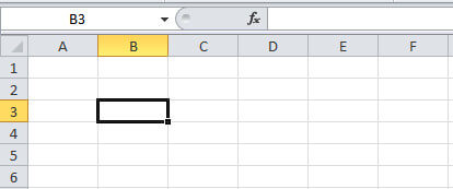
The same rule you have to follow the same naming rule when you select any cell.
Regular Multiple Range Selection
It the method of selecting multiple cells in a certain pattern like square, rectangular, etc. You can select the small and larger area of cells using this method.
To select your pattern, you have followed the steps given below.
Step 1: Go to start cell using mouse or keyboard.
Step 2: Hold ‘shift’ key of the keyboard.
Step 3: Click the last cell
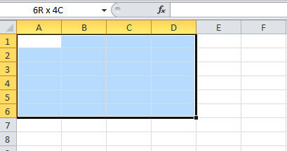
Example: Suppose you want to select the range (A1: D6) as you check in the above image. You have to first go to the cell A1 using your mouse or keyboard. Now, hold the keyboard ‘shift’ key and click the cell D6. This will select the required cell range as given in the above image.
Irregular Multiple Range Selection
An irregular selection is the selection of multiple cells without any patterns. You have to select any numbers of cells in Excel.
To select an irregular pattern, you have to follow the below-given steps:
Step 1: Click on the start cell using the mouse.
Step 2: Hold ‘ctrl’ key of your keyboard.
Step 3: Click the cells you want to select
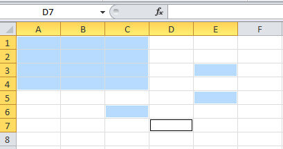
Example: Suppose you want to select the range (A1:C4,C6,E3,E5) given in the above image. Click the start cell or visit start cell using the arrow key of the keyboard. Now, hold the ‘ctrl’ key and click C4. Again click C6, E3, and E5 cells to select with the hold of the ‘ctrl’ keyboard key.
Column Range Selection Using Mouse and Keyboard
If you select all column cell, this also describes the range in Excel. To select all the cells of a column, you can use either your mouse or keyboard depend upon your choice. below are the methods to select all column cell.
Using Mouse
Step 1: Click the column cell name.
Using Keyboard
Step 1: Go the cell to select the column for.
Step 2: Hold ‘ctrl’ and press ‘space’ key of the keyboard.
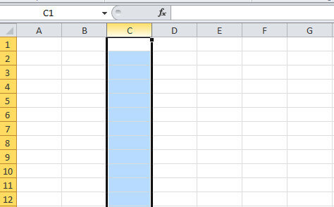
Example Suppose you want to select all the cells of column C given in the above image. You have to just click the column name C using the mouse.
If you want to select using the keyboard, you have to go the column C using arrow key. After that hold the ‘ctrl’ key and press the ‘space’ button of your keyboard. You may also like to read post on how to insert a new column in Excel using a keyboard.
Row Cell Range Selection with Mouse and Keyboard
To select all the cell range of a row, you can use a keyboard or mouse. For mouse use, you have to click the row name given to the left of the cell.
If you want to select all the row cell using only the keyboard, you have to follow the below-given steps.
Step 1: Go to the cell for the row you want using the arrow key.
Step 2: Hold the ‘shift’ key and press ‘space’ button of the keyboard to select the row.
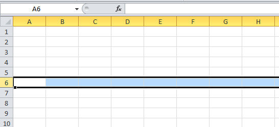
Example: If you want to select the row named 6 as given above. You have to click the name of the row using the mouse. You can also select a row using your keyboard shortcut. Go to any cell of row 6 using your keyboard arrow key. Now, hold the ‘shift’ key and push the ‘space’ bar of your keyboard.`
This will select the row with name 6. You may also like to read post on how to add a new row using MS Excel using the keyboard.
Get Range Selection for A Function of Excel
If you want to select the range from A1 to D7. Go to the cell A1 to start selecting the range. You have to select the range by pressing and holding the keyboard shift key. Now, click the cell D7 to complete the selection.
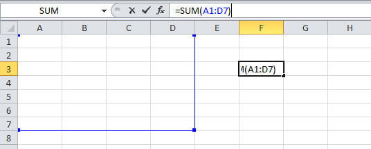
The range after selection showing in the function as SUM(A1:D7). See the image below showing the selection and the output of the sum function.
How to Autofill Numbers for the Selected Cell Range in Excel
Excel comes with many useful features to fill numbers in range. You can autofill range of number in multiple of 1, 2, 3, etc. You have to just grab the plus symbol creates when hovering over the cell. So, let’s create some useful autofill numbers in Excel.
Copy Same Number to Certain Cell Range
Step 1: Go to any cell( e.g.B2) and press the numeric 1 button.
Step 2: Mouse hovers over as indicated arrow location in the below image and holds the left mouse button. You will get a plus(+) sign in place of boxed mouse arrow sign. 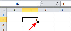
Step 3: Drag the mouse to B7 to get the copy of the number 1 from cell B2 to B7. 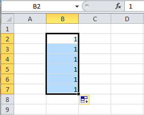
You can copy any number within a certain range using this method.
Autofill Number in Multiples of 2 to Certain Cell Range
Step 1: Go to cell B2, B3 and fill number by pressing button 2,4. In such a manner that 2 is in B2 and 4 is in B3. 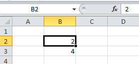
Step 2: Go to cell B2 and press and hold ‘shift’ key. Now, click the B3 cell while holding the ‘shift’ key. This selects the cell B2 and B3. 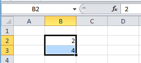
Step 3: Mouse hovers the indicated arrow location given below and holds the left button of the mouse. A plus(+) sign starts to appear in place of boxed mouse arrow sign. 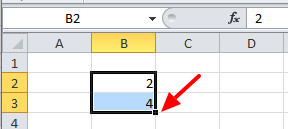
Step 4: Now, you have to just drag the mouse to B8 to get the multiples of 2 from B2 to B8. 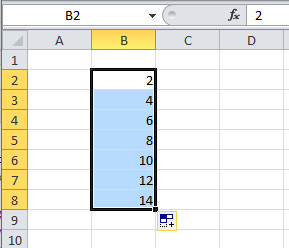
You can fill multiples of any number using the above method. All you have to do is to put the number in multiple first in step 1.
Autofill Dates in the Certain Cell Range in Excel
Step 1: Go to cell B2 and type 1-Aug-95.
Step 2: After typing date, hover over the indicated place given in the image and hold the mouse left button. plus(+) sign showing when you hover over the indicated place. 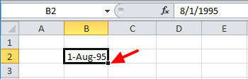
Step 3: Drag the mouse to B11 while holding the mouse left button. This will autofill the date range to a certain cell range. 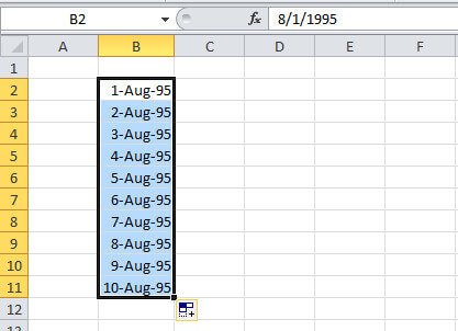
Generate Sequence of Months in Cell Range in Excel
In addition to the above date format, you can also autofill the months. To perform this task and autofill months, follow the given below step-by-step method.
Step 1: Click the cell B2 and type Feb.
Step 2: Now, take your mouse to indicated place as given in the image and hold the mouse left button. A plus(+) sign displays when hovering over the indicated place. 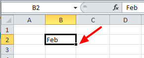
Step 3: You have to just drag the mouse down to the cell B11 with mouse left the button on hold. The selected cell range auto-filled with the sequence of months. 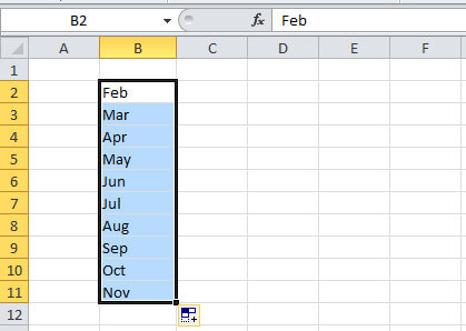
Hope, you like this post of cell range in excel with certain operations. If you have any query regarding the tutorial, please comment below.
Also tell me, what other operations you perform with the range in Excel
Источник
In this tutorial, learn to use Cell Range In Excel with its different operations. A cell range is a collection of two or more cells to use in Excel formula. You can perform operations over single or multiple cells in MS Excel.
What is Cell Range in Excel
A cell range is a group of cells you select to use in functions and perform certain operations. The cell you have to use for the range is the intersection of rows and columns.
You can select multiple cells in a regular and irregular manner. To use the range in any function of Excel, you have to select the cell range with the method given below. You may also like to read post on rows and columns to create a cell in MS Excel.
Select Single Cell Range in Excel
A single cell is the intersection of the row and column of excel. If you click on any cell of the Excel sheet, you can find that it contains a column name and row name.
Let us take an example for the image given below. The below-selected cell is the intersection of column B and row 3. You can read the cell as the combination of row and column name as B3.
The same rule you have to follow the same naming rule when you select any cell.
Regular Multiple Range Selection
It the method of selecting multiple cells in a certain pattern like square, rectangular, etc. You can select the small and larger area of cells using this method.
To select your pattern, you have followed the steps given below.
Step 1: Go to start cell using mouse or keyboard.
Step 2: Hold ‘shift’ key of the keyboard.
Step 3: Click the last cell
Example: Suppose you want to select the range (A1: D6) as you check in the above image. You have to first go to the cell A1 using your mouse or keyboard. Now, hold the keyboard ‘shift’ key and click the cell D6. This will select the required cell range as given in the above image.
Irregular Multiple Range Selection
An irregular selection is the selection of multiple cells without any patterns. You have to select any numbers of cells in Excel.
To select an irregular pattern, you have to follow the below-given steps:
Step 1: Click on the start cell using the mouse.
Step 2: Hold ‘ctrl’ key of your keyboard.
Step 3: Click the cells you want to select
Example: Suppose you want to select the range (A1:C4,C6,E3,E5) given in the above image. Click the start cell or visit start cell using the arrow key of the keyboard. Now, hold the ‘ctrl’ key and click C4. Again click C6, E3, and E5 cells to select with the hold of the ‘ctrl’ keyboard key.
Column Range Selection Using Mouse and Keyboard
If you select all column cell, this also describes the range in Excel. To select all the cells of a column, you can use either your mouse or keyboard depend upon your choice. below are the methods to select all column cell.
Using Mouse
Step 1: Click the column cell name.
Using Keyboard
Step 1: Go the cell to select the column for.
Step 2: Hold ‘ctrl’ and press ‘space’ key of the keyboard.
Example Suppose you want to select all the cells of column C given in the above image. You have to just click the column name C using the mouse.
If you want to select using the keyboard, you have to go the column C using arrow key. After that hold the ‘ctrl’ key and press the ‘space’ button of your keyboard. You may also like to read post on how to insert a new column in Excel using a keyboard.
Row Cell Range Selection with Mouse and Keyboard
To select all the cell range of a row, you can use a keyboard or mouse. For mouse use, you have to click the row name given to the left of the cell.
If you want to select all the row cell using only the keyboard, you have to follow the below-given steps.
Step 1: Go to the cell for the row you want using the arrow key.
Step 2: Hold the ‘shift’ key and press ‘space’ button of the keyboard to select the row.
Example: If you want to select the row named 6 as given above. You have to click the name of the row using the mouse. You can also select a row using your keyboard shortcut. Go to any cell of row 6 using your keyboard arrow key. Now, hold the ‘shift’ key and push the ‘space’ bar of your keyboard.`
This will select the row with name 6. You may also like to read post on how to add a new row using MS Excel using the keyboard.
Get Range Selection for A Function of Excel
If you want to select the range from A1 to D7. Go to the cell A1 to start selecting the range. You have to select the range by pressing and holding the keyboard shift key. Now, click the cell D7 to complete the selection.
The range after selection showing in the function as SUM(A1:D7). See the image below showing the selection and the output of the sum function.
How to Autofill Numbers for the Selected Cell Range in Excel
Excel comes with many useful features to fill numbers in range. You can autofill range of number in multiple of 1, 2, 3, etc. You have to just grab the plus symbol creates when hovering over the cell. So, let’s create some useful autofill numbers in Excel.
Copy Same Number to Certain Cell Range
Step 1: Go to any cell( e.g.B2) and press the numeric 1 button.
Step 2: Mouse hovers over as indicated arrow location in the below image and holds the left mouse button. You will get a plus(+) sign in place of boxed mouse arrow sign.
Step 3: Drag the mouse to B7 to get the copy of the number 1 from cell B2 to B7.
You can copy any number within a certain range using this method.
Autofill Number in Multiples of 2 to Certain Cell Range
Step 1: Go to cell B2, B3 and fill number by pressing button 2,4. In such a manner that 2 is in B2 and 4 is in B3.
Step 2: Go to cell B2 and press and hold ‘shift’ key. Now, click the B3 cell while holding the ‘shift’ key. This selects the cell B2 and B3.
Step 3: Mouse hovers the indicated arrow location given below and holds the left button of the mouse. A plus(+) sign starts to appear in place of boxed mouse arrow sign.
Step 4: Now, you have to just drag the mouse to B8 to get the multiples of 2 from B2 to B8.
You can fill multiples of any number using the above method. All you have to do is to put the number in multiple first in step 1.
Autofill Dates in the Certain Cell Range in Excel
Step 1: Go to cell B2 and type 1-Aug-95.
Step 2: After typing date, hover over the indicated place given in the image and hold the mouse left button. plus(+) sign showing when you hover over the indicated place.
Step 3: Drag the mouse to B11 while holding the mouse left button. This will autofill the date range to a certain cell range.
Generate Sequence of Months in Cell Range in Excel
In addition to the above date format, you can also autofill the months. To perform this task and autofill months, follow the given below step-by-step method.
Step 1: Click the cell B2 and type Feb.
Step 2: Now, take your mouse to indicated place as given in the image and hold the mouse left button. A plus(+) sign displays when hovering over the indicated place.
Step 3: You have to just drag the mouse down to the cell B11 with mouse left the button on hold. The selected cell range auto-filled with the sequence of months.
Hope, you like this post of cell range in excel with certain operations. If you have any query regarding the tutorial, please comment below.
Also tell me, what other operations you perform with the range in Excel
На чтение 18 мин. Просмотров 75.3k.

сэр Артур Конан Дойл
Это большая ошибка — теоретизировать, прежде чем кто-то получит данные
Эта статья охватывает все, что вам нужно знать об использовании ячеек и диапазонов в VBA. Вы можете прочитать его от начала до конца, так как он сложен в логическом порядке. Или использовать оглавление ниже, чтобы перейти к разделу по вашему выбору.
Рассматриваемые темы включают свойство смещения, чтение
значений между ячейками, чтение значений в массивы и форматирование ячеек.
Содержание
- Краткое руководство по диапазонам и клеткам
- Введение
- Важное замечание
- Свойство Range
- Свойство Cells рабочего листа
- Использование Cells и Range вместе
- Свойство Offset диапазона
- Использование диапазона CurrentRegion
- Использование Rows и Columns в качестве Ranges
- Использование Range вместо Worksheet
- Чтение значений из одной ячейки в другую
- Использование метода Range.Resize
- Чтение Value в переменные
- Как копировать и вставлять ячейки
- Чтение диапазона ячеек в массив
- Пройти через все клетки в диапазоне
- Форматирование ячеек
- Основные моменты
Краткое руководство по диапазонам и клеткам
| Функция | Принимает | Возвращает | Пример | Вид |
| Range | адреса ячеек |
диапазон ячеек |
.Range(«A1:A4») | $A$1:$A$4 |
| Cells | строка, столбец |
одна ячейка |
.Cells(1,5) | $E$1 |
| Offset | строка, столбец |
диапазон | .Range(«A1:A2») .Offset(1,2) |
$C$2:$C$3 |
| Rows | строка (-и) | одна или несколько строк |
.Rows(4) .Rows(«2:4») |
$4:$4 $2:$4 |
| Columns | столбец (-цы) |
один или несколько столбцов |
.Columns(4) .Columns(«B:D») |
$D:$D $B:$D |
Введение
Это третья статья, посвященная трем основным элементам VBA. Этими тремя элементами являются Workbooks, Worksheets и Ranges/Cells. Cells, безусловно, самая важная часть Excel. Почти все, что вы делаете в Excel, начинается и заканчивается ячейками.
Вы делаете три основных вещи с помощью ячеек:
- Читаете из ячейки.
- Пишите в ячейку.
- Изменяете формат ячейки.
В Excel есть несколько методов для доступа к ячейкам, таких как Range, Cells и Offset. Можно запутаться, так как эти функции делают похожие операции.
В этой статье я расскажу о каждом из них, объясню, почему они вам нужны, и когда вам следует их использовать.
Давайте начнем с самого простого метода доступа к ячейкам — с помощью свойства Range рабочего листа.
Важное замечание
Я недавно обновил эту статью, сейчас использую Value2.
Вам может быть интересно, в чем разница между Value, Value2 и значением по умолчанию:
' Value2
Range("A1").Value2 = 56

' Value
Range("A1").Value = 56

' По умолчанию используется значение
Range("A1") = 56
Использование Value может усечь число, если ячейка отформатирована, как валюта. Если вы не используете какое-либо свойство, по умолчанию используется Value.
Лучше использовать Value2, поскольку он всегда будет возвращать фактическое значение ячейки.
Свойство Range
Рабочий лист имеет свойство Range, которое можно использовать для доступа к ячейкам в VBA. Свойство Range принимает тот же аргумент, что и большинство функций Excel Worksheet, например: «А1», «А3: С6» и т.д.
В следующем примере показано, как поместить значение в ячейку с помощью свойства Range.
Sub ZapisVYacheiku()

    ' Запишите число в ячейку A1 на листе 1 этой книги
    ThisWorkbook.Worksheets("Лист1").Range("A1").Value2 = 67

    ' Напишите текст в ячейку A2 на листе 1 этой рабочей книги
    ThisWorkbook.Worksheets("Лист1").Range("A2").Value2 = "Иван Петров"

    ' Запишите дату в ячейку A3 на листе 1 этой книги
    ThisWorkbook.Worksheets("Лист1").Range("A3").Value2 = #11/21/2019#

End Sub
Как видно из кода, Range является членом Worksheets, которая, в свою очередь, является членом Workbook. Иерархия такая же, как и в Excel, поэтому должно быть легко понять. Чтобы сделать что-то с Range, вы должны сначала указать рабочую книгу и рабочий лист, которому она принадлежит.
В оставшейся части этой статьи я буду использовать кодовое имя для ссылки на лист.

Следующий код показывает приведенный выше пример с использованием кодового имени рабочего листа, т.е. Лист1 вместо ThisWorkbook.Worksheets («Лист1»).
Sub IspKodImya ()

    ' Запишите число в ячейку A1 на листе 1 этой книги
     Sheet1.Range("A1").Value2 = 67

    ' Напишите текст в ячейку A2 на листе 1 этой рабочей книги
    Sheet1.Range("A2").Value2 = "Иван Петров"

    ' Запишите дату в ячейку A3 на листе 1 этой книги
    Sheet1.Range("A3").Value2 = #11/21/2019#

End Sub
Вы также можете писать в несколько ячеек, используя свойство
Range
Sub ZapisNeskol()

    ' Запишите число в диапазон ячеек
    Sheet1.Range("A1:A10").Value2 = 67

    ' Написать текст в несколько диапазонов ячеек
    Sheet1.Range("B2:B5,B7:B9").Value2 = "Иван Петров"

End Sub
Свойство Cells рабочего листа
У Объекта листа есть другое свойство, называемое Cells, которое очень похоже на Range . Есть два отличия:
- Cells возвращают диапазон только одной ячейки.
- Cells принимает строку и столбец в качестве аргументов.
В приведенном ниже примере показано, как записывать значения
в ячейки, используя свойства Range и Cells.
Sub IspCells()

    ' Написать в А1
    Sheet1.Range("A1").Value2 = 10
    Sheet1.Cells(1, 1).Value2  = 10

    ' Написать в А10
    Sheet1.Range("A10").Value2 = 10
    Sheet1.Cells(10, 1).Value2  = 10

    ' Написать в E1
    Sheet1.Range("E1").Value2 = 10
    Sheet1.Cells(1, 5).Value2  = 10

End Sub
Вам должно быть интересно, когда использовать Cells, а когда Range. Использование Range полезно для доступа к одним и тем же ячейкам при каждом запуске макроса.
Например, если вы использовали макрос для вычисления суммы и
каждый раз записывали ее в ячейку A10, тогда Range подойдет для этой задачи.
Использование свойства Cells полезно, если вы обращаетесь к
ячейке по номеру, который может отличаться. Проще объяснить это на примере.
В следующем коде мы просим пользователя указать номер столбца. Использование Cells дает нам возможность использовать переменное число для столбца.
Sub ZapisVPervuyuPustuyuYacheiku()

    Dim UserCol As Integer

    ' Получить номер столбца от пользователя
    UserCol = Application.InputBox("Пожалуйста, введите номер столбца...", Type:=1)

    ' Написать текст в выбранный пользователем столбец
    Sheet1.Cells(1, UserCol).Value2 = "Иван Петров"

End Sub
В приведенном выше примере мы используем номер для столбца,
а не букву.
Чтобы использовать Range здесь, потребуется преобразовать эти значения в ссылку на
буквенно-цифровую ячейку, например, «С1». Использование свойства Cells позволяет нам
предоставить строку и номер столбца для доступа к ячейке.
Иногда вам может понадобиться вернуть более одной ячейки, используя номера строк и столбцов. В следующем разделе показано, как это сделать.
Использование Cells и Range вместе
Как вы уже видели, вы можете получить доступ только к одной ячейке, используя свойство Cells. Если вы хотите вернуть диапазон ячеек, вы можете использовать Cells с Range следующим образом:
Sub IspCellsSRange()

    With Sheet1
        ' Запишите 5 в диапазон A1: A10, используя свойство Cells
        .Range(.Cells(1, 1), .Cells(10, 1)).Value2 = 5

        ' Диапазон B1: Z1 будет выделен жирным шрифтом
        .Range(.Cells(1, 2), .Cells(1, 26)).Font.Bold = True

    End With

End Sub
Как видите, вы предоставляете начальную и конечную ячейку
диапазона. Иногда бывает сложно увидеть, с каким диапазоном вы имеете дело,
когда значением являются все числа. Range имеет свойство Address, которое
отображает буквенно-цифровую ячейку для любого диапазона. Это может
пригодиться, когда вы впервые отлаживаете или пишете код.
В следующем примере мы распечатываем адрес используемых нами
диапазонов.
Sub PokazatAdresDiapazona()

    ' Примечание. Использование подчеркивания позволяет разделить строки кода.
    With Sheet1

        ' Запишите 5 в диапазон A1: A10, используя свойство Cells
        .Range(.Cells(1, 1), .Cells(10, 1)).Value2 = 5
        Debug.Print "Первый адрес: " _
            + .Range(.Cells(1, 1), .Cells(10, 1)).Address

        ' Диапазон B1: Z1 будет выделен жирным шрифтом
        .Range(.Cells(1, 2), .Cells(1, 26)).Font.Bold = True
        Debug.Print "Второй адрес : " _
            + .Range(.Cells(1, 2), .Cells(1, 26)).Address

    End With

End Sub
В примере я использовал Debug.Print для печати в Immediate Window. Для просмотра этого окна выберите «View» -> «в Immediate Window» (Ctrl + G).


Свойство Offset диапазона
У диапазона есть свойство, которое называется Offset. Термин «Offset» относится к отсчету от исходной позиции. Он часто используется в определенных областях программирования. С помощью свойства «Offset» вы можете получить диапазон ячеек того же размера и на определенном расстоянии от текущего диапазона. Это полезно, потому что иногда вы можете выбрать диапазон на основе определенного условия. Например, на скриншоте ниже есть столбец для каждого дня недели. Учитывая номер дня (т.е. понедельник = 1, вторник = 2 и т.д.). Нам нужно записать значение в правильный столбец.

Сначала мы попытаемся сделать это без использования Offset.
' Это Sub тесты с разными значениями
Sub TestSelect()

    ' Понедельник
    SetValueSelect 1, 111.21
    ' Среда
    SetValueSelect 3, 456.99
    ' Пятница
    SetValueSelect 5, 432.25
    ' Воскресение
    SetValueSelect 7, 710.17

End Sub

' Записывает значение в столбец на основе дня
Public Sub SetValueSelect(lDay As Long, lValue As Currency)

    Select Case lDay
        Case 1: Sheet1.Range("H3").Value2 = lValue
        Case 2: Sheet1.Range("I3").Value2 = lValue
        Case 3: Sheet1.Range("J3").Value2 = lValue
        Case 4: Sheet1.Range("K3").Value2 = lValue
        Case 5: Sheet1.Range("L3").Value2 = lValue
        Case 6: Sheet1.Range("M3").Value2 = lValue
        Case 7: Sheet1.Range("N3").Value2 = lValue
    End Select

End Sub
Как видно из примера, нам нужно добавить строку для каждого возможного варианта. Это не идеальная ситуация. Использование свойства Offset обеспечивает более чистое решение.
' Это Sub тесты с разными значениями
Sub TestOffset()

    DayOffSet 1, 111.01
    DayOffSet 3, 456.99
    DayOffSet 5, 432.25
    DayOffSet 7, 710.17

End Sub

Public Sub DayOffSet(lDay As Long, lValue As Currency)

    ' Мы используем значение дня с Offset, чтобы указать правильный столбец
    Sheet1.Range("G3").Offset(, lDay).Value2 = lValue

End Sub
Как видите, это решение намного лучше. Если количество дней увеличилось, нам больше не нужно добавлять код. Чтобы Offset был полезен, должна быть какая-то связь между позициями ячеек. Если столбцы Day в приведенном выше примере были случайными, мы не могли бы использовать Offset. Мы должны были бы использовать первое решение.
Следует иметь в виду, что Offset сохраняет размер диапазона. Итак .Range («A1:A3»).Offset (1,1) возвращает диапазон B2:B4. Ниже приведены еще несколько примеров использования Offset.
Sub IspOffset()

    ' Запись в В2 - без Offset
    Sheet1.Range("B2").Offset().Value2 = "Ячейка B2"

    ' Написать в C2 - 1 столбец справа
    Sheet1.Range("B2").Offset(, 1).Value2 = "Ячейка C2"

    ' Написать в B3 - 1 строка вниз
    Sheet1.Range("B2").Offset(1).Value2 = "Ячейка B3"

    ' Запись в C3 - 1 столбец справа и 1 строка вниз
    Sheet1.Range("B2").Offset(1, 1).Value2 = "Ячейка C3"

    ' Написать в A1 - 1 столбец слева и 1 строка вверх
    Sheet1.Range("B2").Offset(-1, -1).Value2 = "Ячейка A1"

    ' Запись в диапазон E3: G13 - 1 столбец справа и 1 строка вниз
    Sheet1.Range("D2:F12").Offset(1, 1).Value2 = "Ячейки E3:G13"

End Sub
Использование диапазона CurrentRegion
CurrentRegion возвращает диапазон всех соседних ячеек в данный диапазон. На скриншоте ниже вы можете увидеть два CurrentRegion. Я добавил границы, чтобы прояснить CurrentRegion.

Строка или столбец пустых ячеек означает конец CurrentRegion.
Вы можете вручную проверить
CurrentRegion в Excel, выбрав диапазон и нажав Ctrl + Shift + *.
Если мы возьмем любой диапазон
ячеек в пределах границы и применим CurrentRegion, мы вернем диапазон ячеек во
всей области.
Например:
Range («B3»). CurrentRegion вернет диапазон B3:D14
Range («D14»). CurrentRegion вернет диапазон B3:D14
Range («C8:C9»). CurrentRegion вернет диапазон B3:D14 и так далее
Как пользоваться
Мы получаем CurrentRegion следующим образом
' CurrentRegion вернет B3:D14 из приведенного выше примера
Dim rg As Range
Set rg = Sheet1.Range("B3").CurrentRegion
Только чтение строк данных
Прочитать диапазон из второй строки, т.е. пропустить строку заголовка.
' CurrentRegion вернет B3:D14 из приведенного выше примера
Dim rg As Range
Set rg = Sheet1.Range("B3").CurrentRegion

' Начало в строке 2 - строка после заголовка
Dim i As Long
For i = 2 To rg.Rows.Count
    ' текущая строка, столбец 1 диапазона
    Debug.Print rg.Cells(i, 1).Value2
Next i
Удалить заголовок
Удалить строку заголовка (т.е. первую строку) из диапазона. Например, если диапазон — A1:D4, это возвратит A2:D4
' CurrentRegion вернет B3:D14 из приведенного выше примера
Dim rg As Range
Set rg = Sheet1.Range("B3").CurrentRegion

' Удалить заголовок
Set rg = rg.Resize(rg.Rows.Count - 1).Offset(1)

' Начните со строки 1, так как нет строки заголовка
Dim i As Long
For i = 1 To rg.Rows.Count
    ' текущая строка, столбец 1 диапазона
    Debug.Print rg.Cells(i, 1).Value2
Next i
Использование Rows и Columns в качестве Ranges
Если вы хотите что-то сделать со всей строкой или столбцом,
вы можете использовать свойство «Rows и
Columns» на рабочем листе. Они оба принимают один параметр — номер строки
или столбца, к которому вы хотите получить доступ.
Sub IspRowIColumns()

    ' Установите размер шрифта столбца B на 9
    Sheet1.Columns(2).Font.Size = 9

    ' Установите ширину столбцов от D до F
    Sheet1.Columns("D:F").ColumnWidth = 4

    ' Установите размер шрифта строки 5 до 18
    Sheet1.Rows(5).Font.Size = 18

End Sub
Использование Range вместо Worksheet
Вы также можете использовать Cella, Rows и Columns, как часть Range, а не как часть Worksheet. У вас может быть особая необходимость в этом, но в противном случае я бы избегал практики. Это делает код более сложным. Простой код — твой друг. Это уменьшает вероятность ошибок.
Код ниже выделит второй столбец диапазона полужирным. Поскольку диапазон имеет только две строки, весь столбец считается B1:B2
Sub IspColumnsVRange()

    ' Это выделит B1 и B2 жирным шрифтом.
    Sheet1.Range("A1:C2").Columns(2).Font.Bold = True

End Sub
Чтение значений из одной ячейки в другую
В большинстве примеров мы записали значения в ячейку. Мы
делаем это, помещая диапазон слева от знака равенства и значение для размещения
в ячейке справа. Для записи данных из одной ячейки в другую мы делаем то же
самое. Диапазон назначения идет слева, а диапазон источника — справа.
В следующем примере показано, как это сделать:
Sub ChitatZnacheniya()

    ' Поместите значение из B1 в A1
    Sheet1.Range("A1").Value2 = Sheet1.Range("B1").Value2

    ' Поместите значение из B3 в лист2 в ячейку A1
    Sheet1.Range("A1").Value2 = Sheet2.Range("B3").Value2

    ' Поместите значение от B1 в ячейки A1 до A5
    Sheet1.Range("A1:A5").Value2 = Sheet1.Range("B1").Value2

    ' Вам необходимо использовать свойство «Value», чтобы прочитать несколько ячеек
    Sheet1.Range("A1:A5").Value2 = Sheet1.Range("B1:B5").Value2

End Sub
Как видно из этого примера, невозможно читать из нескольких ячеек. Если вы хотите сделать это, вы можете использовать функцию копирования Range с параметром Destination.
Sub KopirovatZnacheniya()

    ' Сохранить диапазон копирования в переменной
    Dim rgCopy As Range
    Set rgCopy = Sheet1.Range("B1:B5")

    ' Используйте это для копирования из более чем одной ячейки
    rgCopy.Copy Destination:=Sheet1.Range("A1:A5")

    ' Вы можете вставить в несколько мест назначения
    rgCopy.Copy Destination:=Sheet1.Range("A1:A5,C2:C6")

End Sub
Функция Copy копирует все, включая формат ячеек. Это тот же результат, что и ручное копирование и вставка выделения. Подробнее об этом вы можете узнать в разделе «Копирование и вставка ячеек»
Использование метода Range.Resize
При копировании из одного диапазона в другой с использованием присваивания (т.е. знака равенства) диапазон назначения должен быть того же размера, что и исходный диапазон.
Использование функции Resize позволяет изменить размер
диапазона до заданного количества строк и столбцов.
Например:
Sub ResizePrimeri()

    ' Печатает А1
    Debug.Print Sheet1.Range("A1").Address

    ' Печатает A1:A2
    Debug.Print Sheet1.Range("A1").Resize(2, 1).Address

    ' Печатает A1:A5
    Debug.Print Sheet1.Range("A1").Resize(5, 1).Address

    ' Печатает A1:D1
    Debug.Print Sheet1.Range("A1").Resize(1, 4).Address

    ' Печатает A1:C3
    Debug.Print Sheet1.Range("A1").Resize(3, 3).Address

End Sub
Когда мы хотим изменить наш целевой диапазон, мы можем
просто использовать исходный размер диапазона.
Другими словами, мы используем количество строк и столбцов
исходного диапазона в качестве параметров для изменения размера:
Sub Resize()

    Dim rgSrc As Range, rgDest As Range

    ' Получить все данные в текущей области
    Set rgSrc = Sheet1.Range("A1").CurrentRegion

      ' Получить диапазон назначения
    Set rgDest = Sheet2.Range("A1")
    Set rgDest = rgDest.Resize(rgSrc.Rows.Count, rgSrc.Columns.Count)

    rgDest.Value2 = rgSrc.Value2

End Sub
Мы можем сделать изменение размера в одну строку, если нужно:
Sub Resize2()

    Dim rgSrc As Range

    ' Получить все данные в ткущей области
    Set rgSrc = Sheet1.Range("A1").CurrentRegion

    With rgSrc
        Sheet2.Range("A1").Resize(.Rows.Count, .Columns.Count) = .Value2
    End With

End Sub
Чтение Value в переменные
Мы рассмотрели, как читать из одной клетки в другую. Вы также можете читать из ячейки в переменную. Переменная используется для хранения значений во время работы макроса. Обычно вы делаете это, когда хотите манипулировать данными перед тем, как их записать. Ниже приведен простой пример использования переменной. Как видите, значение элемента справа от равенства записывается в элементе слева от равенства.
Sub IspVar()

    ' Создайте
    Dim val As Integer

    ' Читать число из ячейки
    val = Sheet1.Range("A1").Value2

    ' Добавить 1 к значению
    val = val + 1

    ' Запишите новое значение в ячейку
    Sheet1.Range("A2").Value2 = val

End Sub
Для чтения текста в переменную вы используете переменную
типа String.
Sub IspVarText()

    ' Объявите переменную типа string
    Dim sText As String

    ' Считать значение из ячейки
    sText = Sheet1.Range("A1").Value2

    ' Записать значение в ячейку
    Sheet1.Range("A2").Value2 = sText

End Sub
Вы можете записать переменную в диапазон ячеек. Вы просто
указываете диапазон слева, и значение будет записано во все ячейки диапазона.
Sub VarNeskol()

    ' Считать значение из ячейки
    Sheet1.Range("A1:B10").Value2 = 66

End Sub
Вы не можете читать из нескольких ячеек в переменную. Однако
вы можете читать массив, который представляет собой набор переменных. Мы
рассмотрим это в следующем разделе.
Как копировать и вставлять ячейки
Если вы хотите скопировать и вставить диапазон ячеек, вам не
нужно выбирать их. Это распространенная ошибка, допущенная новыми пользователями
VBA.
Вы можете просто скопировать ряд ячеек, как здесь:
Range("A1:B4").Copy Destination:=Range("C5")
При использовании этого метода копируется все — значения,
форматы, формулы и так далее. Если вы хотите скопировать отдельные элементы, вы
можете использовать свойство PasteSpecial
диапазона.
Работает так:
Range("A1:B4").Copy
Range("F3").PasteSpecial Paste:=xlPasteValues
Range("F3").PasteSpecial Paste:=xlPasteFormats
Range("F3").PasteSpecial Paste:=xlPasteFormulas
В следующей таблице приведен полный список всех типов вставок.
| Виды вставок |
| xlPasteAll |
| xlPasteAllExceptBorders |
| xlPasteAllMergingConditionalFormats |
| xlPasteAllUsingSourceTheme |
| xlPasteColumnWidths |
| xlPasteComments |
| xlPasteFormats |
| xlPasteFormulas |
| xlPasteFormulasAndNumberFormats |
| xlPasteValidation |
| xlPasteValues |
| xlPasteValuesAndNumberFormats |
Чтение диапазона ячеек в массив
Вы также можете скопировать значения, присвоив значение
одного диапазона другому.
Range("A3:Z3").Value2 = Range("A1:Z1").Value2
Значение диапазона в этом примере считается вариантом массива. Это означает, что вы можете легко читать из диапазона ячеек в массив. Вы также можете писать из массива в диапазон ячеек. Если вы не знакомы с массивами, вы можете проверить их в этой статье.
В следующем коде показан пример использования массива с
диапазоном.
Sub ChitatMassiv()

    ' Создать динамический массив
    Dim StudentMarks() As Variant

    ' Считать 26 значений в массив из первой строки
    StudentMarks = Range("A1:Z1").Value2

    ' Сделайте что-нибудь с массивом здесь

    ' Запишите 26 значений в третью строку
    Range("A3:Z3").Value2 = StudentMarks

End Sub
Имейте в виду, что массив, созданный для чтения, является
двумерным массивом. Это связано с тем, что электронная таблица хранит значения
в двух измерениях, то есть в строках и столбцах.
Пройти через все клетки в диапазоне
Иногда вам нужно просмотреть каждую ячейку, чтобы проверить значение.
Вы можете сделать это, используя цикл For Each, показанный в следующем коде.
Sub PeremeschatsyaPoYacheikam()

    ' Пройдите через каждую ячейку в диапазоне
    Dim rg As Range
    For Each rg In Sheet1.Range("A1:A10,A20")
        ' Распечатать адрес ячеек, которые являются отрицательными
        If rg.Value < 0 Then
            Debug.Print rg.Address + " Отрицательно."
        End If
    Next

End Sub
Вы также можете проходить последовательные ячейки, используя
свойство Cells и стандартный цикл For.
Стандартный цикл более гибок в отношении используемого вами
порядка, но он медленнее, чем цикл For Each.
Sub PerehodPoYacheikam()

    ' Пройдите клетки от А1 до А10
    Dim i As Long
    For i = 1 To 10
        ' Распечатать адрес ячеек, которые являются отрицательными
        If Range("A" & i).Value < 0 Then
            Debug.Print Range("A" & i).Address + " Отрицательно."
        End If
    Next

    ' Пройдите в обратном порядке, то есть от A10 до A1
    For i = 10 To 1 Step -1
        ' Распечатать адрес ячеек, которые являются отрицательными
        If Range("A" & i) < 0 Then
            Debug.Print Range("A" & i).Address + " Отрицательно."
        End If
    Next

End Sub
Форматирование ячеек
Иногда вам нужно будет отформатировать ячейки в электронной
таблице. Это на самом деле очень просто. В следующем примере показаны различные
форматы, которые можно добавить в любой диапазон ячеек.
Sub FormatirovanieYacheek()

    With Sheet1

        ' Форматировать шрифт
        .Range("A1").Font.Bold = True
        .Range("A1").Font.Underline = True
        .Range("A1").Font.Color = rgbNavy

        ' Установите числовой формат до 2 десятичных знаков
        .Range("B2").NumberFormat = "0.00"
        ' Установите числовой формат даты
        .Range("C2").NumberFormat = "dd/mm/yyyy"
        ' Установите формат чисел на общий
        .Range("C3").NumberFormat = "Общий"
        ' Установить числовой формат текста
        .Range("C4").NumberFormat = "Текст"

        ' Установите цвет заливки ячейки
        .Range("B3").Interior.Color = rgbSandyBrown

        ' Форматировать границы
        .Range("B4").Borders.LineStyle = xlDash
        .Range("B4").Borders.Color = rgbBlueViolet

    End With

End Sub
Основные моменты
Ниже приводится краткое изложение основных моментов
- Range возвращает диапазон ячеек
- Cells возвращают только одну клетку
- Вы можете читать из одной ячейки в другую
- Вы можете читать из диапазона ячеек в другой диапазон ячеек.
- Вы можете читать значения из ячеек в переменные и наоборот.
- Вы можете читать значения из диапазонов в массивы и наоборот
- Вы можете использовать цикл For Each или For, чтобы проходить через каждую ячейку в диапазоне.
- Свойства Rows и Columns позволяют вам получить доступ к диапазону ячеек этих типов
Appearance of a Cell Range
A symmetrical cell range can appear as below. The notation for this range is (A1:C6); from upper left cell A1 to bottom right cell C6.

Irregular Cell Ranges
Irregular cell ranges, like in the image below, also occur. The notation for this range is (A1:C6;E2;E6;C7;C9).

A Cell Range Within a Formula
A cell range can be used inside a formula, for example to calculate the sum of the values within the selected cells. The notation for the sum of all values in cell range (A1:C6) is =SUM(A1:C6).

Range Issues
Larger spreadsheets are usually stuffed with formulas based on cell ranges. When spreadsheets are edited or expanded over time, different types of range issues may occur. These issues are usually hard to detect, but they can be very risky! We’ve seen big numbers and large sums of money ‘disappear’ because of range issues.
PerfectXL detects different types of range issues, like references to empty cells, interrupted formula ranges, merged cells, references to merged cells, unexpected ranges and ranges in which unexpected shifts occur.