
Содержание
- Define and use names in formulas
- Name a cell
- Define names from a selected range
- Use names in formulas
- Manage names in your workbook with Name Manager
- Name a cell
- Define names from a selected range
- Use names in formulas
- Manage names in your workbook with Name Manager
- Need more help?
- What is a cell in Excel?
- Which data can enter into cell
- How to identify cell number?
- Enter data into the cell
- Delete cell data
- Delete cell
- Cell range
- How to select multiple cells
- 1. Continues selection
- 2. Scattered selection
- Cut, copy, and paste the cells data
- Copy and paste the cell data
- Cut and paste the cell data
- How to increase the size of cell
- Feedback
- Help Others, Please Share
- Learn Latest Tutorials
- Preparation
- Trending Technologies
- B.Tech / MCA
- Javatpoint Services
- Training For College Campus
- Naming cells in Microsoft Office Excel
- Why name cells in Excel
- How to name cells in Excel
- Changing a cell name in the name box:
- Defining a cell name:
Define and use names in formulas
By using names, you can make your formulas much easier to understand and maintain. You can define a name for a cell range, function, constant, or table. Once you adopt the practice of using names in your workbook, you can easily update, audit, and manage these names.

Name a cell
In the Name Box, type a name.
To reference this value in another table, type th equal sign (=) and the Name, then select Enter.
Define names from a selected range
Select the range you want to name, including the row or column labels.
Select Formulas > Create from Selection.
In the Create Names from Selection dialog box, designate the location that contains the labels by selecting the Top row, Left column, Bottom row, or Right column check box.
Excel names the cells based on the labels in the range you designated.
Use names in formulas
Select a cell and enter a formula.
Place the cursor where you want to use the name in that formula.
Type the first letter of the name, and select the name from the list that appears.
Or, select Formulas > Use in Formula and select the name you want to use.
Manage names in your workbook with Name Manager
On the ribbon, go to Formulas > Name Manager. You can then create, edit, delete, and find all the names used in the workbook.
Name a cell
In the Name Box, type a name.
Define names from a selected range
Select the range you want to name, including the row or column labels.
Select Formulas > Create from Selection.
In the Create Names from Selection dialog box, designate the location that contains the labels by selecting the Top row, Left column, Bottom row, or Right column check box.
Excel names the cells based on the labels in the range you designated.
Use names in formulas
Select a cell and enter a formula.
Place the cursor where you want to use the name in that formula.
Type the first letter of the name, and select the name from the list that appears.
Or, select Formulas > Use in Formula and select the name you want to use.
Manage names in your workbook with Name Manager
On the Ribbon, go to Formulas > Defined Names > Name Manager. You can then create, edit, delete, and find all the names used in the workbook.
In Excel for the web, you can use the named ranges you’ve defined in Excel for Windows or Mac. Select a name from the Name Box to go to the range’s location, or use the Named Range in a formula.
For now, creating a new Named Range in Excel for the web is not available.
Need more help?
You can always ask an expert in the Excel Tech Community or get support in the Answers community.
Источник
What is a cell in Excel?
A cell is an essential part of MS-Excel. It is an object of Excel worksheets. Whenever you open Excel, the Excel worksheet contains cells to store the information in them. You enter content and your data into these cells. Cells are the building blocks of the Excel worksheet. So, you should know every single point about it.
In the Excel worksheet, a cell is a rectangular-shaped box. It is a small unit of the Excel spreadsheet. There are around 17 billion cells in an Excel worksheet, which are united together in horizontal and vertical lines.
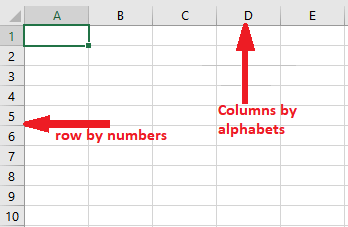
An Excel worksheet contains cells in rows and columns. Rows are labeled as numbers and columns as alphabets. It means the rows are identified by numbers and columns by alphabets.
Which data can enter into cell
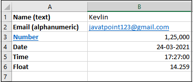
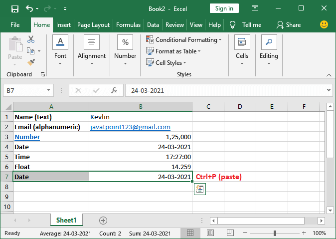
Excel consists of a group of cells in a worksheet. You can enter data in any of these cells. Excel allows the user to enter any type of data in Excel cells, such as numeric, text, date, and time data. Whatever you enter in a cell, it appears inside the cell and as well as in the formula bar.
Double-tap on any of a cell to make it editable and write the data in it. In Excel, you can enter any type of data in Excel cells, such as number, string, text, date, time, etc. In addition, the users can also perform operations on it.
How to identify cell number?
In Excel, you can easily identify the cell number you are currently in. You can either find the cell number inside the Name box or also from row and column headers.
The highlighted row and column in the header is the cell number when a cell is selected. See the screenshot below:
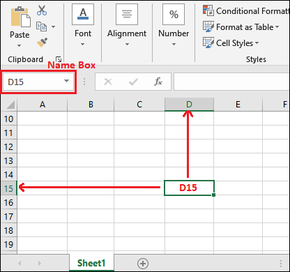
Else see the cell number inside the Name box of the currently selected cell and get the cell number, e.g., D15.
Enter data into the cell
To enter the data/information into a cell, double-tap on any cell to make it editable and write the data in it. Let’s understand with an example.
Delete cell data
Select the cell along with data inside it and either press Backspace or Delete button to delete the content of the cell. It will delete one letter at a time means 1 tap backspace/delete will delete only one letter of that cell.
You can also delete cell data in one go. For this, select the cell data and then either press the Backspace or Delete button. The selected cell content will be deleted.
You can also use this Delete button to delete the content of multiple cells. For this, you have to select cells with data whose data you want to delete and press the Delete key on your keyboard. The data of the selected cells will be deleted.
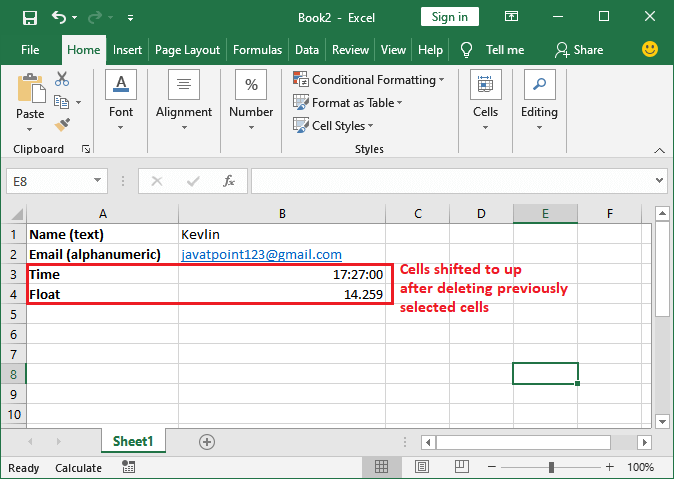
Delete cell
There is a huge difference between deleting the cell data or deleting a cell itself. So, don’t be confused between them. To delete the cells, you have to perform a bit different steps, as we are discussing below:
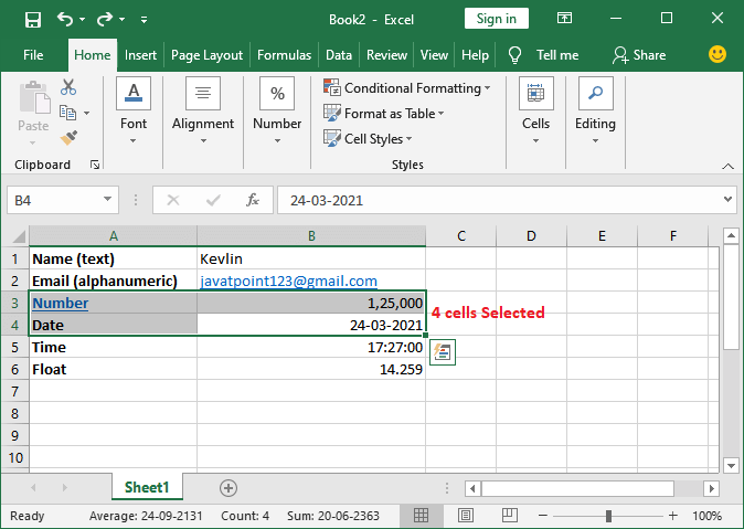
Step 1: Select one or more cells, which you want to delete. E.g., A3, A4, and B3, B4.
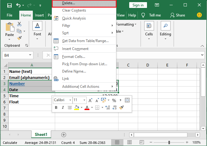
Step 2: Right-click any of the selected cells and click on the Delete command present inside the list.
Step 3: Mark the relevant radio button and click on the OK button. We have chosen to Shift cells up option to shift the remaining cells data of the selected column to the upper row.
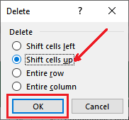
Step 4: The selected cells will be deleted and the remaining cells will shift up at the place of deleted cells.
Cell range
Cell range is one, which has a starting and ending point. When the multiple cells are selected in a sequence, it is called as cell range. Cell range shows from start cell to end cell. Selected cells must be in sequence without any gap in selection.
For example,
Cell range A1:A8
Cell A1 to A8 is selected in this range. It means that total 8 cells are selected.
Cell range A1:B8
Cell A1 to A8 and B1 to B8 are selected in this cell range. It means that total 16 cells are selected.
How to select multiple cells
Sometimes, there is a need to select a large range of cell data in an Excel sheet. You can easily select a larger group of cells or a cell range in two ways. Either with mouse or shift and arrow key.
1. Continues selection
Firstly, we will show you a contiguous selection of multiple cells using both methods.
- Select cells with mouse
Click on a cell, hold the mouse left key and drag until you got select all needed cells.
- Select cells with Shift and arrow key
There is one more way selecting multiple cells at one time. You can use the Shift key with arrow keys (choose direction) to select multiple cells.
Firstly, click on one cell in the Excel worksheet. Keep pressing the shift key and use the required arrow key with it according to selection to select the multiple cells.
2. Scattered selection
Excel also allows to select multiple cells from different rows and columns without following any contiguous selection range process as above. We can do it only using the Ctrl key.
- Select scattered cells with the CTRL key
Excel provides a way to select two or more cells of different rows and different columns. You can use the CTRL key to hold the selection and then choose the cells to select.
Remember that only those cells will be selected which has some data. Blank cells cannot be selected even using the Ctrl key.
Cut, copy, and paste the cells data
Cut, copy, and paste are the most used operations of every tool. Excel allows its users to copy or cut the content from one place and paste it to another cell in Excel.
Excel also provides shortcut commands for these operations. CTRL + C for copy, CTRL + P for paste the copied content, and CTRL + X for cut is used in Excel. These shortcut keys are the same for almost every tool.
Copy and paste the cell data
Step 1: Select the cell whose data you want to copy and press the CTRL+C command to copy the data.
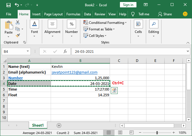
Step 2: Now, go to that where you want to paste the copied data and press the CTRL+P shortcut command to place the data there.
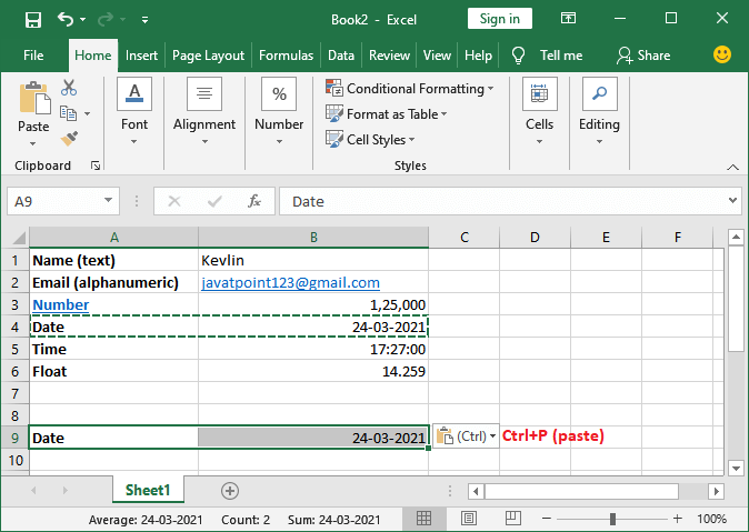
Step 3: Your data has been copied from one cell and pasted to another one.
Cut and paste the cell data
Step 1: Select the cell whose data you want to cut and press the CTRL+X command.
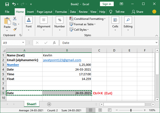
Step 2: Now, go to the cell where you want to paste the cut data and press the CTRL+P shortcut command to place the data there.
Step 3: Your data has been placed from one cell and pasted to another one.
How to increase the size of cell
In Excel, you can increase the size of cells in following ways:
- Increase the height of the row from row header
- Increase the width of the column from column header
- Merge the two or more cells to enhance the cell size
- Increase the font size to make the cell bigger
You can use any of these methods accordingly as needed.
Feedback


Learn Latest Tutorials
Python Design Patterns
Preparation


Trending Technologies
B.Tech / MCA
Javatpoint Services
JavaTpoint offers too many high quality services. Mail us on [email protected], to get more information about given services.
- Website Designing
- Website Development
- Java Development
- PHP Development
- WordPress
- Graphic Designing
- Logo
- Digital Marketing
- On Page and Off Page SEO
- PPC
- Content Development
- Corporate Training
- Classroom and Online Training
- Data Entry
Training For College Campus
JavaTpoint offers college campus training on Core Java, Advance Java, .Net, Android, Hadoop, PHP, Web Technology and Python. Please mail your requirement at [email protected]
Duration: 1 week to 2 week
Источник
Naming cells in Microsoft Office Excel
 Microsoft Office is a suite of office applications that was initially released in 1990. One of these applications included in the suite is Excel, which is a spreadsheet program that is commonly used for data management, as well as for creating graphs and tables. Did you know that the cells that make up a spreadsheet in Excel can be named for easy identification? This feature is available on all versions of Excel, including Office Web Apps and the versions that come with Office 365.
Like other spreadsheet applications, Microsoft Excel documents are based on cells that can be arranged into rows and columns. It is within these cells that data is entered when creating a worksheet for various functions including data management and computations, etc. Each cell in the spreadsheet has a corresponding name, which is identified by its column letter and row number.
For instance, the cell under column A that belongs to row 1 has the default name A1. You will see this in the name box, which is located on the upper left side of the spreadsheet, next to the formula bar. This name can actually be changed however.
Why name cells in Excel
As mentioned, the default name for each cell in an Excel spreadsheet is based on the relevant column and row. One of the reasons why you may want to change this name is to make it easier to find what you are looking for, especially when there’s a lot of information in a particular spreadsheet. For instance, if you name a particular cell ‘Total’, searching for this word is much faster than scrolling through the spreadsheet to find the correct cell or trying to remember its specific column and row.
This is also the case when creating formulas for computations. Instead of using the cells’ column letter and row number, it’s more convenient to use a name that you can easily understand. For example, naming one cell ‘GrossIncome’ and the other one ‘Deductions’ makes it easier for you to compute net income by subtracting Deductions from GrossIncome for the result.
Another benefit of naming cells is that it is easier for other users to understand. If you are sharing the spreadsheet or workbook with other colleagues or business associates, using cell names that are easy for everyone to identify reduces potential confusion.
How to name cells in Excel
Naming cells in Excel can be done in two ways. The first is by changing the name directly on the name box and the other one is by defining names under the Formulas menu. The difference is that when naming a cell through the define name feature of the menu you can select its specific scope.
This determines where the specific name will be recognized as having the same value, such as in the entire workbook or in a specific spreadsheet only. Changing the name in the name box will automatically determine the workbook as its scope rather than the whole spreadsheet.
Changing a cell name in the name box:
- Select the cell that you want to name.
- Go to the name box and type the name you prefer.
- Hit enter on your keyboard.
Defining a cell name:
- Select the cell that you wish to name.
- Click the Formulas menu.
- Choose Define Name.
- Type the name of the cell in the new window that pops up.
- Select the Scope.
- Click OK.
Remember that a cell name should not contain any spaces. The uppercase and lowercase letters R and C are also not available as cell names, since they represent column and row. Furthermore, aside from letters, the first character of a cell name can also be a backslash or an underscore. The rest can be a combination of letters, underscores, periods and numbers, which can be up to 255 characters.
If you have further questions about changing the cell name in Excel, please don’t hesitate to give us a call.
Источник
A cell reference or cell address is a combination of a column letter and a row number that identifies a cell on a worksheet. For example, A1 refers to the cell at the intersection of column A and row 1; B2 refers to the second cell in column B, and so on.
Contents
- 1 What is the function of cell address?
- 2 What is the cell address in a formula called?
- 3 What is the cell address of the first cell in Excel?
- 4 What is cell address give example?
- 5 What is a cell reference?
- 6 What are the three types of cell references in Excel?
- 7 How do you reference a cell reference in Excel?
- 8 What is the cell address of the last cell in a worksheet?
- 9 Is the address of column 27 and 30?
- 10 What is the first and last cell address in Excel?
- 11 What is cell address explain its types?
- 12 What is the difference between cell and cell address?
- 13 What is a cell reference class 9?
- 14 What is cell referencing Class 7?
- 15 What is cell and cell reference?
- 16 What is address example?
- 17 How is an address formatted?
- 18 What is referencing and its types?
- 19 What is B $3 in Excel?
- 20 What are Excel cell references by default?
What is the function of cell address?
The ADDRESS function returns the address for a cell based on a given row and column number. For example, =ADDRESS(1,1) returns $A$1. ADDRESS can return a relative, mixed, or absolute reference, and can be used to construct a cell reference inside a formula.
What is the cell address in a formula called?
cell reference
Answer. The cell address in a formula is also called cell reference.
What is the cell address of the first cell in Excel?
=ADDRESS(1,1) – returns the address of the first cell (i.e. the cell at the intersection of the first row and first column) as an absolute cell reference $A$1. =ADDRESS(1,1,4) – returns the address of the first cell as a relative cell reference A1.
What is cell address give example?
A reference is a cell’s address. It identifies a cell or range of cells by referring to the column letter and row number of the cell(s). For example, A1 refers to the cell at the intersection of column A and row 1. The reference tells Formula One for Java to use the contents of the referenced cell(s) in the formula.
What is a cell reference?
A cell reference refers to a cell or a range of cells on a worksheet and can be used in a formula so that Microsoft Office Excel can find the values or data that you want that formula to calculate.
What are the three types of cell references in Excel?
Relative, Absolute and Mixed
A key element of a formula is the cell reference, and there are three types: Relative. Absolute. Mixed.
How do you reference a cell reference in Excel?
Use cell references in a formula
- Click the cell in which you want to enter the formula.
- In the formula bar. , type = (equal sign).
- Do one of the following, select the cell that contains the value you want or type its cell reference.
- Press Enter.
What is the cell address of the last cell in a worksheet?
Answer: The intersection of row 1048576 and column XFD is called XFD1048576.
Is the address of column 27 and 30?
So, it will be called AA33.
What is the first and last cell address in Excel?
Answer: =ADDRESS(1,1) – returns the address of the first cell (i.e. the cell at the intersection of the first row and first column) as an absolute cell reference $A$1. =ADDRESS(1,1,4) – returns the address of the first cell as a relative cell reference A1.
What is cell address explain its types?
There are two types of cell references: relative and absolute. Relative and absolute references behave differently when copied and filled to other cells. Relative references change when a formula is copied to another cell. Absolute references, on the other hand, remain constant no matter where they are copied.
What is the difference between cell and cell address?
A cell is a single box in the excel spreadsheet which has only one row and one column address. In Excel, the rows are listed as numbers and the columns are named as letters.For example, if we select a 3×3 area in excel starting from the cell B2, the address of the cell range will be shown as B2:D4.
What is a cell reference class 9?
Cell Reference
A reference identifies a cell or a range of cells on a worksheet and tells MS Excel where to look for value or data to be used in a formula. Using reference, we can use data present in different parts of a worksheet or on a different worksheet or another workbook.
What is cell referencing Class 7?
Cell referencing helps us to identify the behaviour of a cell address in a formula when it is copied from one to another cell. The three types of the referencing are: i. RELATIVE REFERENCING: In this type of referencing both parts of the cell address are not fixed. For example: B3*C3.
What is cell and cell reference?
A cell reference in Excel refers to the value of a different cell or cell range on the current worksheet or a different worksheet within the spreadsheet. A cell reference can be used as a variable in a formula.
What is address example?
Frequency: The definition of an address is a written or verbal statement, or the physical location of something. An example of an address is the President’s Inaugural speech. 123 Main Street, New York, NY 10030 is an example of an address.
How is an address formatted?
The name of the sender should be placed on the first line. If you’re sending from a business, you would list the company name on the next line. Next, you should write out the building number and street name. The final line should have the city, state and ZIP code for the address.
What is referencing and its types?
Explanation:
- Relative referencing : In relative referencing, both column part and row part are not fixed .
- Absolute referencing : In absolute referencing, both column part and row part are fixed.
- Mixed referencing : In mixed referencing,either column part or row part is fixed.
Otherwise, it does change. That is, the $ sign “anchors” a row number or column letter when you copy it.
How to Use Absolute and Relative Cell References in Excel Formulas.
| =B3 | tap {F4} to get: |
|---|---|
| =B$3 | tap {F4} to get: |
| =$B3 | tap {F4} to get: |
| =B3 | (etc) |
What are Excel cell references by default?
By default, a cell reference is a relative reference, which means that the reference is relative to the location of the cell. If, for example, you refer to cell A2 from cell C2, you are actually referring to a cell that is two columns to the left (C minus A)—in the same row (2).
![]()
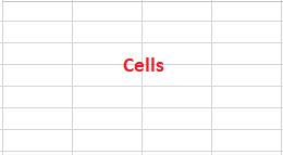
Excel Cell

Cell is an Object of Excel Sheet to enter information. It represents with Column Name followed by Row Number. The address of the First Cell in the Excel Sheet is A1 (A is the First Column and 1 is the first Row in Excel sheet). The format of an Excel spread sheet looks like a Table and the intersection of Rows and Columns formats blocks (boxes), each of these small blocks are called Cells in Excel.
How to enter data in a Cell
You can select any Cell in the Excel and press F2 function key to make the Cell editable. Then enter the data using your keyboard in the Cell. You can also double click on a Cell to make it to data entry mode.
What kind of information we can enter in a Cell
We can enter text, numbers, dates, formulas, images, chars, icons and special characters in Excel Cells. We can perform mathematical and logical operations based on our requirements. We can also format the Cell with font styles, colors, number formats,etc.
| Type of Data | Approach to Enter in Excel |
|---|---|
| Enter Date in excel | Use Shortcut key CTRL+ ; (Control and Semicolon) to enter date in Excel. |
| Enter formula in excel | Double Click on any Cell and start with = and enter your formula expression. |
| Enter time in excel | You can use TIMEVALUE(time_text) function to accept the Time. Or you can formate the cell into required time format “h:mm:ss AM/PM”, and enter time value in the cell. |
| Enter today’s date in excel | You can use Ctrl+ ; Shortcut key to enter todats Date in Excel. |
| Enter a checkmark in excel | You can use Char(252) function or Alt+0252 to enter Check Box Character and Change Font of the Cell to Wingdings. |
| Enter a drop down list in excel | Goto Data tab in the Ribbon menu and Clcik on the Data Validation Command to enter Drop down List. |
| Enter 20 digit number in excel | Start with ‘ (apostrophe) and enter the number or format the cell as Text, the number will save as string. |
| Enter a checkbox in excel | Use alt code 0252 and format font to Wingdings. Alternatively, use Symbol command in Insert menu. |
Merge Split (Un Merge) Cells
We have following options and tools in the Excel to merge and unmerge (split) the cells in Excel. You use it based on your requirement.
How to Merge Cells in Excel ?
Follow the below steps to merge the Cells in Excel:
- Select the required range of cells in the sheet
- Go to Home tab in the Ribbon Menu
- Press the ‘Merge Cells‘ Command to merge the Cells.
How to Split Merged Cells in Excel?
Follow the below steps to split the merged Cells in Excel:
- Select the merged cell in the sheet
- Go to Home tab in the Ribbon Menu
- Press the ‘Merge Cells‘ Command to split the cells.
How to Merge Data in Two or More Cells in Excel?
Follow the below steps to merge the data in multiple Cells in Excel:
- You can use the Concatenate Formula to Merge the Cells. For example, =Concatenate(A1,B1)
- You can use concatenate operator & to merge the cell data. For example, =A1&B1
How to Change Excel Cell Size?
You can follow the one of the method to increase the size of the cell in Excel.
- By increasing the width of the column
- Increase the height of the Row
- Increase the font size to make the cell bigger
- merge multiple Cells to make one large size cell
How to Split Data in a Cell in Excel?
Follow the below steps to split the data in a Cell into multiple Cells and Columns:
- Select the required Cell or Column to Split
- Go to Data tab in the Excel Ribbon menu
- Click on the ‘Text to Column’ command in the Data tools group
- Choose and Delimited character or fixed with option to split the data.
How to Extract the Text from Excel Cell?
Follow the below steps to split the data in a Cell into multiple Cells and Columns:
- Select the required Cell or Column to Split
- Go to Data tab in the Excel Ribbon menu
- Click on the ‘Text to Column’ command in the Data tools group
- Choose and Delimited character or fixed with option to split the data.
Lock and Unlock Cells in Excel
We need to protect our data in Excel to hide it from others users. We can use built in Excel tools to lock and unlock the Cells.
How to Lock Excel Cells?
You can lock entire sheet or specific range of cells in the Excel. Follow the below steps to lock the required Cells in the Excel.
- Select the required range of cells to lock (By default Excel cells are locked)
- Then Go to Review Tab in the Excel Ribbon menu
- Click on the ‘Protect Sheet’ command available in the Protect Group.
- Choose the Required things to restrict and enter the password to protect
- And confirm it and press OK to lock it.
How to Un Lock Excel Cells?
Follow the below steps to unlock the cells in Excel. Make sure you have the password to unlock the sheet.
- Go to Review Tab in the Excel Ribbon menu
- Click on the ‘Unprotect Sheet’ command available in the Protect Group.
- Enter the password to un lock the sheet
- Select the required range of cells to un lock.
- Right Click on it and press Format Cells command
- Un select the Locked check mark in the Protection Tab
- Now you can reset the password (if required)
Removing Text from Cells
You can select the required cells to remove the text, press delete key on your keyboard. Excel stores verity of data in Cells, you can follow the below methods to remove the required data from Cells.
| Data | Approach to remove |
|---|---|
| Text | Click Delete Button or Press the Clear Contents command from Editing Tools in Home Tab. |
| Format | Press Clear Formats command from Editiong tools to delete only Formats of the Cells. |
| Comments | Press Clear Comments command from Editiong tools to delete only Comments in the Cells. |
| Delete Everything | Press Clear All command from Editiong tools to delete everything in Cells. |
How to Remove Specific Text From Excel Cell
You can follow the one the following methods to remove specific text from Excel Cells.
- One Cell: You can double click on the cell and select the required text and press delete button from your keyboard.
- Multiple Cells or Columns: You can select entire range of cells and use find and Replace Dialog (Ctrl+H) to remove the specific text (Find What:= your text, Leave blank in the Replace with: text box)
- Part Of Text Criteria: You can use formulas (Mid, Find,Len,Trim) to remove the text based on specific criteria or to Remove Part Of Text From Excel Cell.
How to New Line In Excel Cell
Press Alt+Enter to add new line in Excel. You can use Char(10) with Excel Formula.
Fill Color in Excel Cells
You can fill single or multiple color to set the background colors of the Excel Cells. You fill Solid color or Gradients Color.
- Standard Colors: You can select any cell and go to the Home tab and click on the fill color control (color bucket icon) to set the standard colors in Excel.
- Theme Colors: You can use the one of the colors from Excel Theme Styles, All the cells will change automatically when you change color theme.
- Gradient Colors: You can set Multiple color shading within a single cell using Gradient Effects in Excel. Click on the Format Cells command from the right click menu. And go to Fill Tab and press the Fill effects to set the Cells gradient colors. You can use this option to Split a cell in excel with two or three colors
Cell in Excel Object Model
Cell is a child object of Worksheet. Worksheet is a collection of all cells in the worksheet. Portion of the spreadsheet (One or group of Cells) is called Range in Excel. Here is the Object Model of Excel Cell.

How to Refer a Cell
We use Column Name followed by Row Number to refer a Cell in Excel. For example, C5 is the intersection area of Column C and Row 5. Here C5 is called the address of the Cell. There are two types of methods we can use to refer a Cell.
- Relative Reference: The address of the Cell will change relatively while performing the Excel Operations. It is the default reference type and we can refer as A1 to refer the first cell of a sheet.
- Absolute Reference: The address of the Cell will be fixed and will not change while performing Excel Operations like Copying, Dragging and Auto filling the Cells. We can put $ symbol to make the Row or Column Absolute. For Example, $C$5 is the absolute reference of the cell A5.
We refer the cells to use the data of any cell in other cells and objects. We can use Relative reference, Absolute reference or both combined based on our requirement.
For Example:
=$D$5: will lock both Column and Row, Both Column and Rows are Absolute.
=$D5: will lock Column and will not lock the Row, Column is Absolute and Row is Relative.
=D$5: will lock Row and will not lock the Column, Row is Absolute and Column is Relative.
= D5: Both Column and Rows are Relative.
What is an Active Cell?
A Cell which is currently selected in the Active Sheet of the Active Window is called Active Cell. ActiveCell is an Object of the Worksheet Object , we can use ActiveCell to deal with the currently selected cell of the active worksheet.
For Example:
- We can Enter the data in the Active Cell by typing from keyboard. You can use ActiveCell.Value=10 in Excel Macros.
- We can Format the Active Cell using builtin tools, You can format using Excel Macros like ActiveCell.Font.Bold

© Copyright 2012 – 2020 | Excelx.com | All Rights Reserved
Page load link
 Microsoft Office is a suite of office applications that was initially released in 1990. One of these applications included in the suite is Excel, which is a spreadsheet program that is commonly used for data management, as well as for creating graphs and tables. Did you know that the cells that make up a spreadsheet in Excel can be named for easy identification? This feature is available on all versions of Excel, including Office Web Apps and the versions that come with Office 365.
Like other spreadsheet applications, Microsoft Excel documents are based on cells that can be arranged into rows and columns. It is within these cells that data is entered when creating a worksheet for various functions including data management and computations, etc. Each cell in the spreadsheet has a corresponding name, which is identified by its column letter and row number.
For instance, the cell under column A that belongs to row 1 has the default name A1. You will see this in the name box, which is located on the upper left side of the spreadsheet, next to the formula bar. This name can actually be changed however.
Why name cells in Excel
As mentioned, the default name for each cell in an Excel spreadsheet is based on the relevant column and row. One of the reasons why you may want to change this name is to make it easier to find what you are looking for, especially when there’s a lot of information in a particular spreadsheet. For instance, if you name a particular cell ‘Total’, searching for this word is much faster than scrolling through the spreadsheet to find the correct cell or trying to remember its specific column and row.
This is also the case when creating formulas for computations. Instead of using the cells’ column letter and row number, it’s more convenient to use a name that you can easily understand. For example, naming one cell ‘GrossIncome’ and the other one ‘Deductions’ makes it easier for you to compute net income by subtracting Deductions from GrossIncome for the result.
Another benefit of naming cells is that it is easier for other users to understand. If you are sharing the spreadsheet or workbook with other colleagues or business associates, using cell names that are easy for everyone to identify reduces potential confusion.
How to name cells in Excel
Naming cells in Excel can be done in two ways. The first is by changing the name directly on the name box and the other one is by defining names under the Formulas menu. The difference is that when naming a cell through the define name feature of the menu you can select its specific scope.
This determines where the specific name will be recognized as having the same value, such as in the entire workbook or in a specific spreadsheet only. Changing the name in the name box will automatically determine the workbook as its scope rather than the whole spreadsheet.
Changing a cell name in the name box:
- Select the cell that you want to name.
- Go to the name box and type the name you prefer.
- Hit enter on your keyboard.
Defining a cell name:
- Select the cell that you wish to name.
- Click the Formulas menu.
- Choose Define Name.
- Type the name of the cell in the new window that pops up.
- Select the Scope.
- Click OK.
Remember that a cell name should not contain any spaces. The uppercase and lowercase letters R and C are also not available as cell names, since they represent column and row. Furthermore, aside from letters, the first character of a cell name can also be a backslash or an underscore. The rest can be a combination of letters, underscores, periods and numbers, which can be up to 255 characters.
If you have further questions about changing the cell name in Excel, please don’t hesitate to give us a call.
Updated: 12/31/2020 by
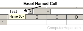
To create a named cell in Microsoft Excel, select the cell and click the Name Box next to the formula bar, as shown in the image. This bar has the current cell location printed in it. For example, if you’re in cell A1, it should currently say A1 in the Name Box. In the Name Box, type the name you want to name the cell and press Enter.
Once a cell is named, you can refer to this cell in a formula, chart, or anything else that uses cell references. For example, let’s assume you named a cell profits. When creating a new formula, you could type =sum(B10+profits) to add cell B10 plus the value in the profits cell.
Tip
When naming a cell or range, it can only be one word with no spaces.
Tip
In Excel, use the shortcut key Ctrl+F3 to open the Name Manager. In the Name Manager, you can create, edit, and delete any Excel names. Once a name is created, you can use the shortcut key F3 to insert any name.
Why is it beneficial to name cells in a spreadsheet?
It is easier to use the name of a cell instead of the cell reference. For example, it’s easier to remember «profits» (as mentioned earlier) instead of the cell containing the profits value.