
Excel for Microsoft 365 Excel for Microsoft 365 for Mac Excel for the web Excel 2021 Excel 2021 for Mac Excel 2019 Excel 2019 for Mac Excel 2016 Excel 2016 for Mac Excel 2013 Excel for iPad Excel for iPhone Excel for Android tablets Excel 2010 Excel 2007 Excel for Mac 2011 Excel for Android phones Excel Starter 2010 More…Less
The CELL function returns information about the formatting, location, or contents of a cell. For example, if you want to verify that a cell contains a numeric value instead of text before you perform a calculation on it, you can use the following formula:
=IF(CELL(«type»,A1)=»v»,A1*2,0)
This formula calculates A1*2 only if cell A1 contains a numeric value, and returns 0 if A1 contains text or is blank.
Note: Formulas that use CELL have language-specific argument values and will return errors if calculated using a different language version of Excel. For example, if you create a formula containing CELL while using the Czech version of Excel, that formula will return an error if the workbook is opened using the French version. If it is important for others to open your workbook using different language versions of Excel, consider either using alternative functions or allowing others to save local copies in which they revise the CELL arguments to match their language.
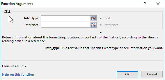
Syntax
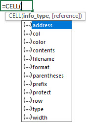
CELL(info_type, [reference])
The CELL function syntax has the following arguments:
|
Argument |
Description |
|---|---|
|
info_type Required |
A text value that specifies what type of cell information you want to return. The following list shows the possible values of the Info_type argument and the corresponding results. |
|
reference Optional |
The cell that you want information about. If omitted, the information specified in the info_type argument is returned for cell selected at the time of calculation. If the reference argument is a range of cells, the CELL function returns the information for active cell in the selected range. Important: Although technically reference is optional, including it in your formula is encouraged, unless you understand the effect its absence has on your formula result and want that effect in place. Omitting the reference argument does not reliably produce information about a specific cell, for the following reasons:
|
info_type values
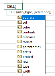
The following list describes the text values that can be used for the info_type argument. These values must be entered in the CELL function with quotes (» «).
|
info_type |
Returns |
|---|---|
|
«address» |
Reference of the first cell in reference, as text. |
|
«col» |
Column number of the cell in reference. |
|
«color» |
The value 1 if the cell is formatted in color for negative values; otherwise returns 0 (zero). Note: This value is not supported in Excel for the web, Excel Mobile, and Excel Starter. |
|
«contents» |
Value of the upper-left cell in reference; not a formula. |
|
«filename» |
Filename (including full path) of the file that contains reference, as text. Returns empty text («») if the worksheet that contains reference has not yet been saved. Note: This value is not supported in Excel for the web, Excel Mobile, and Excel Starter. |
|
«format» |
Text value corresponding to the number format of the cell. The text values for the various formats are shown in the following table. Returns «-» at the end of the text value if the cell is formatted in color for negative values. Returns «()» at the end of the text value if the cell is formatted with parentheses for positive or all values. Note: This value is not supported in Excel for the web, Excel Mobile, and Excel Starter. |
|
«parentheses» |
The value 1 if the cell is formatted with parentheses for positive or all values; otherwise returns 0. Note: This value is not supported in Excel for the web, Excel Mobile, and Excel Starter. |
|
«prefix» |
Text value corresponding to the «label prefix» of the cell. Returns single quotation mark (‘) if the cell contains left-aligned text, double quotation mark («) if the cell contains right-aligned text, caret (^) if the cell contains centered text, backslash () if the cell contains fill-aligned text, and empty text («») if the cell contains anything else. Note: This value is not supported in Excel for the web, Excel Mobile, and Excel Starter. |
|
«protect» |
The value 0 if the cell is not locked; otherwise returns 1 if the cell is locked. Note: This value is not supported in Excel for the web, Excel Mobile, and Excel Starter. |
|
«row» |
Row number of the cell in reference. |
|
«type» |
Text value corresponding to the type of data in the cell. Returns «b» for blank if the cell is empty, «l» for label if the cell contains a text constant, and «v» for value if the cell contains anything else. |
|
«width» |
Returns an array with 2 items. The 1st item in the array is the column width of the cell, rounded off to an integer. Each unit of column width is equal to the width of one character in the default font size. The 2nd item in the array is a Boolean value, the value is TRUE if the column width is the default or FALSE if the width has been explicitly set by the user. Note: This value is not supported in Excel for the web, Excel Mobile, and Excel Starter. |
CELL format codes
The following list describes the text values that the CELL function returns when the Info_type argument is «format» and the reference argument is a cell that is formatted with a built-in number format.
|
If the Excel format is |
The CELL function returns |
|---|---|
|
General |
«G» |
|
0 |
«F0» |
|
#,##0 |
«,0» |
|
0.00 |
«F2» |
|
#,##0.00 |
«,2» |
|
$#,##0_);($#,##0) |
«C0» |
|
$#,##0_);[Red]($#,##0) |
«C0-« |
|
$#,##0.00_);($#,##0.00) |
«C2» |
|
$#,##0.00_);[Red]($#,##0.00) |
«C2-« |
|
0% |
«P0» |
|
0.00% |
«P2» |
|
0.00E+00 |
«S2» |
|
# ?/? or # ??/?? |
«G» |
|
m/d/yy or m/d/yy h:mm or mm/dd/yy |
«D4» |
|
d-mmm-yy or dd-mmm-yy |
«D1» |
|
d-mmm or dd-mmm |
«D2» |
|
mmm-yy |
«D3» |
|
mm/dd |
«D5» |
|
h:mm AM/PM |
«D7» |
|
h:mm:ss AM/PM |
«D6» |
|
h:mm |
«D9» |
|
h:mm:ss |
«D8» |
Note: If the info_type argument in the CELL function is «format» and you later apply a different format to the referenced cell, you must recalculate the worksheet (press F9) to update the results of the CELL function.
Examples
Need more help?
You can always ask an expert in the Excel Tech Community or get support in the Answers community.
See Also
Change the format of a cell
Create or change a cell reference
ADDRESS function
Add, change, find or clear conditional formatting in a cell
Need more help?
Want more options?
Explore subscription benefits, browse training courses, learn how to secure your device, and more.
Communities help you ask and answer questions, give feedback, and hear from experts with rich knowledge.
Содержание
- CELL function
- Syntax
- info_type values
- CELL format codes
- CELL Function Examples – Excel & Google Sheets
- CELL Function Overview
- CELL function Syntax and inputs:
- How to use the CELL Function in Excel
- Overall View of Info_types
- Color Info_type
- Format Info_type
- Parentheses Info_type
- Prefix Info_type
- Protect Info_type
- Type Info_type
- Create Hyperlink to Lookup Using Address
- Retrieve File Path
- Retrieve File Name
- Retrieve Sheet Name
- CELL Function in Google Sheets
- Additional Notes
- Excel CELL function with formula examples
- Excel CELL function — syntax and basic uses
- Info_type values
- Format codes
- How to use the CELL function in Excel — formula examples
- Get address of the lookup result
- Make a hyperlink to the lookup result (first match)
- Get different parts of the file path
- Workbook name
- Worksheet name
- Path to the file
- Path and file name
CELL function
The CELL function returns information about the formatting, location, or contents of a cell. For example, if you want to verify that a cell contains a numeric value instead of text before you perform a calculation on it, you can use the following formula:
This formula calculates A1*2 only if cell A1 contains a numeric value, and returns 0 if A1 contains text or is blank.
Note: Formulas that use CELL have language-specific argument values and will return errors if calculated using a different language version of Excel. For example, if you create a formula containing CELL while using the Czech version of Excel, that formula will return an error if the workbook is opened using the French version. If it is important for others to open your workbook using different language versions of Excel, consider either using alternative functions or allowing others to save local copies in which they revise the CELL arguments to match their language.
Syntax
The CELL function syntax has the following arguments:
A text value that specifies what type of cell information you want to return. The following list shows the possible values of the Info_type argument and the corresponding results.
The cell that you want information about.
If omitted, the information specified in the info_type argument is returned for cell selected at the time of calculation. If the reference argument is a range of cells, the CELL function returns the information for active cell in the selected range.
Important: Although technically reference is optional, including it in your formula is encouraged, unless you understand the effect its absence has on your formula result and want that effect in place. Omitting the reference argument does not reliably produce information about a specific cell, for the following reasons:
In automatic calculation mode, when a cell is modified by a user the calculation may be triggered before or after the selection has progressed, depending on the platform you’re using for Excel. For example, Excel for Windows currently triggers calculation before selection changes, but Excel for the web triggers it afterward.
When Co-Authoring with another user who makes an edit, this function will report your active cell rather than the editor’s.
Any recalculation, for instance pressing F9, will cause the function to return a new result even though no cell edit has occurred.
info_type values
The following list describes the text values that can be used for the info_type argument. These values must be entered in the CELL function with quotes (» «).
Reference of the first cell in reference, as text.
Column number of the cell in reference.
The value 1 if the cell is formatted in color for negative values; otherwise returns 0 (zero).
Note: This value is not supported in Excel for the web, Excel Mobile, and Excel Starter.
Value of the upper-left cell in reference; not a formula.
Filename (including full path) of the file that contains reference, as text. Returns empty text («») if the worksheet that contains reference has not yet been saved.
Note: This value is not supported in Excel for the web, Excel Mobile, and Excel Starter.
Text value corresponding to the number format of the cell. The text values for the various formats are shown in the following table. Returns «-» at the end of the text value if the cell is formatted in color for negative values. Returns «()» at the end of the text value if the cell is formatted with parentheses for positive or all values.
Note: This value is not supported in Excel for the web, Excel Mobile, and Excel Starter.
The value 1 if the cell is formatted with parentheses for positive or all values; otherwise returns 0.
Note: This value is not supported in Excel for the web, Excel Mobile, and Excel Starter.
Text value corresponding to the «label prefix» of the cell. Returns single quotation mark (‘) if the cell contains left-aligned text, double quotation mark («) if the cell contains right-aligned text, caret (^) if the cell contains centered text, backslash () if the cell contains fill-aligned text, and empty text («») if the cell contains anything else.
Note: This value is not supported in Excel for the web, Excel Mobile, and Excel Starter.
The value 0 if the cell is not locked; otherwise returns 1 if the cell is locked.
Note: This value is not supported in Excel for the web, Excel Mobile, and Excel Starter.
Row number of the cell in reference.
Text value corresponding to the type of data in the cell. Returns «b» for blank if the cell is empty, «l» for label if the cell contains a text constant, and «v» for value if the cell contains anything else.
Returns an array with 2 items.
The 1st item in the array is the column width of the cell, rounded off to an integer. Each unit of column width is equal to the width of one character in the default font size.
The 2nd item in the array is a Boolean value, the value is TRUE if the column width is the default or FALSE if the width has been explicitly set by the user.
Note: This value is not supported in Excel for the web, Excel Mobile, and Excel Starter.
CELL format codes
The following list describes the text values that the CELL function returns when the Info_type argument is «format» and the reference argument is a cell that is formatted with a built-in number format.
Источник
CELL Function Examples – Excel & Google Sheets
Download the example workbook
This Tutorial demonstrates how to use the Excel CELL Function in Excel to get information about a cell.
CELL Function Overview
The CELL Function Returns information about a cell. Color, filename, contents, format, row, etc.
To use the CELL Excel Worksheet Function, select a cell and type:
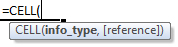
(Notice how the formula inputs appear)
CELL function Syntax and inputs:
info_type – Text indicating what cell information you would like to return.
reference – The cell reference that you want information about.
How to use the CELL Function in Excel
The CELL Function returns information about the formatting, location, or contents of cell.
As seen above, the CELL Function returns all kinds of information from cell B3.
If you type =CELL(, you will be able to see 12 different types of information to retrieve.
Here are additional outputs of the CELL Function:
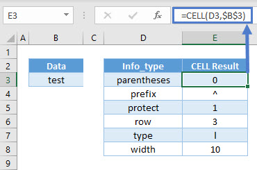
Overall View of Info_types
Some of the info_types are pretty straightforward and retrieves what you asked for, while the rest will be explained in the next few sections because of the complexity.
| Info_type | What it retrieves? |
| “address” | The cell reference/address. |
| “col” | The column number. |
| “color” | * |
| “contents” | The value itself or result of the formula. |
| “filename” | The full path, filename, and extension in square brackets, and sheet name. |
| “format” | * |
| “parentheses” | * |
| “prefix” | * |
| “protect” | * |
| “row” | The row number. |
| “type” | * |
| “width” | The column width rounded to the nearest integer. |
* Explained in the next few sections.
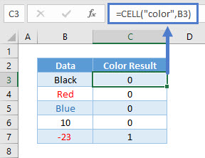
Color Info_type
Color will show all results as 0 unless the cell is formatted with color for negative values. The latter will show as 1.
Format Info_type
Format shows the number format of the cell, but it might not be what you expect.
There are many kinds of different variations with formatting, but here are some guidelines to figure it out:
- “G” is for General, “C” for Currency, “P” for Percentage, “S” for Scientific (not shown above), “D” for Date.
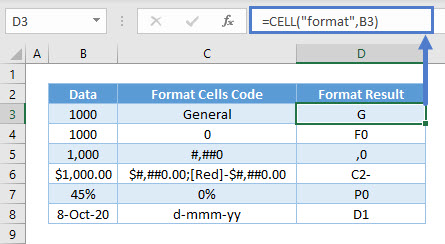
- If the digits are with numbers, currencies, and percentages; it represents the decimal places. Eg. “F0” means 0 decimals in cell D4, and “C2-” means 2 decimals in cell D6. “D1” in cell D8 is simply a type of date format (there are D1 to D9 for different kinds of date and time formats).
- A comma at the beginning is for thousand separators (“,0” in cell D5 for eg).
- A minus sign is for formatting negative values with a color (“C2-” in cell D6 for eg).
Here are other examples of date formats and for scientific.
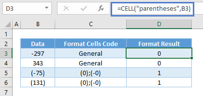
Parentheses Info_type
Parentheses shows 1 if the cell is formatted with parentheses (either or both positive and negative). Otherwise, it shows 0.
Prefix Info_type
Prefix results in various symbols depending on how the text is aligned in the cell.
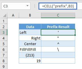
As seen above, a left alignment of the text is a single quote in cell C3.
A right alignment of the text shows double quotes in cell C4.
A center alignment of the text shows caret in cell C5.
A fill alignment of the text shows backslash in cell C6.
Numbers (cell C7 and C8) show as blank regardless of alignment.
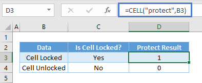
Protect Info_type
Protect results in 1 if the cell is locked, and 0 if it’s unlocked.
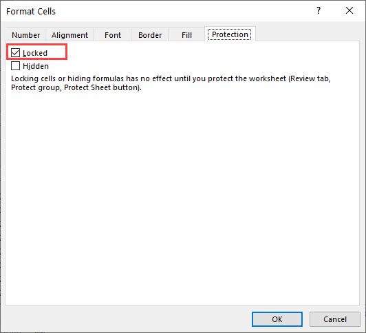
Do note that all cells are locked by default. That is why you can’t edit any cells after you protect it. To unlock it, right-click on a cell and choose Format Cells.
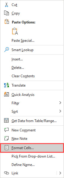
Go to the Protection tab and you can uncheck “Locked” to unlock the cell.
Type Info_type
Type results in three different alphabets dependent on the data type in the cell.
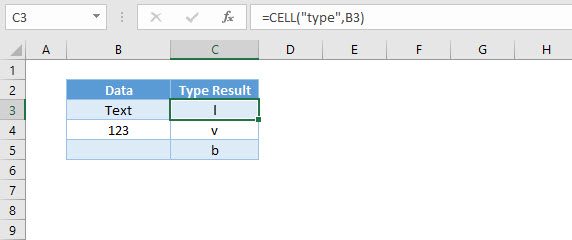
“l” stands for label in cell C3.
“v” stands for value in cell C4.
“b” stands for blank in cell C5.
Create Hyperlink to Lookup Using Address
You can use the CELL Function along with HYPERLINK and INDEX / MATCH to hyperlink to a lookup result:
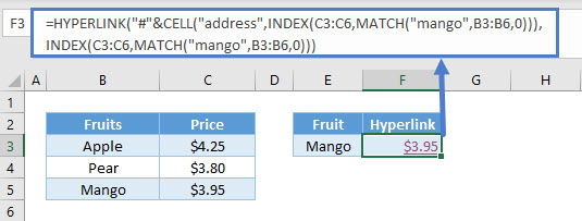
The INDEX and MATCH formula retrieves the price of Mango in cell C5: $3.95. The CELL Function, with “address” returns the cell location. The HYPERLINK function then creates the hyperlink.
Retrieve File Path
To retrieve the file path where the particular file is stored, you can use:
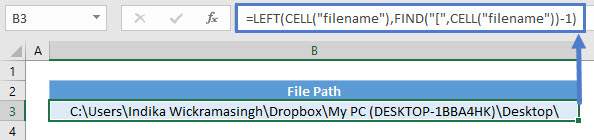
Since the filename will be the same using any cell reference, you can omit it. Use FIND function to obtain the position where “[“ starts and minus 1 to allow LEFT function to retrieve the characters before that.
Retrieve File Name
To retrieve the file name, you can use:
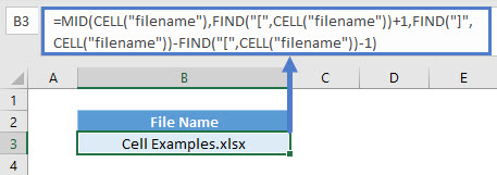
This uses a similar concept as above where FIND function obtains the position where “[“ starts and retrieves the characters after that. To know how many characters to extract, it uses the position of “]” minus “[“ and minus 1 as it includes the position of “]”.
Retrieve Sheet Name
To retrieve the sheet name, you can use:
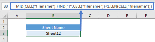
Again, it’s similar to the above where FIND function obtains the position where “]“ starts and retrieves the characters after that. To know how many characters to extract, it uses the total length of what “filename” info_type returns.
CELL Function in Google Sheets
The CELL function works similarly in Google Sheets. It just doesn’t have the full range of info_type. It only includes “address”, “col”, “color”, “contents”, “prefix”, “row”, “type”, and “width”.
Additional Notes
The CELL Function returns information about a cell. The information that can be returned relates to cell location, formatting and contents.
Enter the type of information you want then enter the cell reference for the cell you want information about.
Источник
Excel CELL function with formula examples
 by Svetlana Cheusheva, updated on March 16, 2023
The tutorial shows how to use the CELL function in Excel to retrieve various information about a cell such as cell address, contents, formatting, location, and more.
How do you usually get specific information about a cell in Excel? Someone would check it visually with their own eyes, others would use the ribbon options. But a faster and more reliable way is to use the Excel CELL function. Among other things, it can tell you whether a cell is protected or not, bring a number format and column width, show a full path to the workbook that contains the cell, and a lot more.
Excel CELL function — syntax and basic uses
The CELL function in Excel returns various information about a cell such as cell contents, formatting, location, etc.
The syntax of the CELL function is as follows:
- info_type (required) — the type of information to return about the cell.
- reference (optional) — the cell for which to retrieve information. Typically, this argument is a single cell. If supplied as a range of cells, the formula returns information about the upper left cell of the range. If omitted, the information is returned for the last changed cell on the sheet.
Info_type values
The following table shows all possible values for the info_type argument accepted by the Excel CELL function.
| Info_type | Description |
| «address» | The address of the cell, returned as text. |
| «col» | The column number of the cell. |
| «color» | The number 1 if the cell is color-formatted for negative values; otherwise 0 (zero). |
| «contents» | The value of the cell. If the cell contains a formula, its calculated value is returned. |
| «filename» | The filename and full path to the workbook that contains the cell, returned as text. If the workbook containing the cell has not been saved yet, an empty string («») is returned. |
| «format» | A special code that corresponds to the number format of the cell. For more information, please see Format codes. |
| «parentheses» | The number 1 if the cell is formatted with parentheses for positive or all values; otherwise 0. |
| «prefix» | One of the following values depending on how text is aligned in the cell:
For numeric values, an empty string (blank cell) is returned regardless of the alignment. |
| «protect» | The number 1 if the cell is locked; 0 if the cell is not locked.
Please note, «locked» is not the same as «protected». The Locked attributed is pre-selected for all cells in Excel by default. To protect a cell from editing or deleting, you need to protect the worksheet. |
| «row» | The row number of the cell. |
| «type» | One of the following text values corresponding to the data type in the cell:
|
| «width» | The column width of the cell rounded to the nearest integer. Please see Excel column width for more information about the width units. |
- All info_types retrieve information about the first (upper-left) cell in the reference argument.
- The «filename», «format», «parentheses», «prefix», «protect» and «width» values are not supported in Excel Online, Excel Mobile, and Excel Starter.
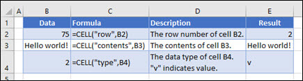
As an example, let’s use the Excel CELL function to return different properties of cell A2 that contains the text value in the General format:
| A | B | C | D | |
|---|---|---|---|---|
| 1 | Data | Formula | Result | Description |
| 2 | Apple | =CELL(«address», $A$2) | $A$2 | Cell address as an absolute reference |
| 3 | =CELL(«col», $A$2) | 1 | Column 1 | |
| 4 | =CELL(«color», $A$2) | 0 | Cell is not formatted with color | |
| 5 | =CELL(«contents», $A$2) | Apple | Cell value | |
| 6 | =CELL(«format»,$A$2) | G | General format | |
| 7 | =CELL(«parentheses», $A$2) | 0 | The cell is not formatted with parentheses | |
| 8 | =CELL(«prefix», $A$2) | ^ | Centered text | |
| 9 | =CELL(«protect», $A$2) | 1 | The cell is locked (the default state) | |
| 10 | =CELL(«row», $A$2) | 2 | Row 2 | |
| 11 | =CELL(«type», $A$2) | l | A text constant | |
| 12 | =CELL(«width», $A$2) | 3 | Column width rounded to an integer |
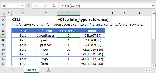
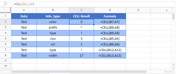
The screenshot shows the results of another Excel CELL formula, which returns different information about cell A2 based on the info_type value in column B. For this, we enter the following formula in C2 and then drag it down to copy the formula to other cells:
=CELL(B2, $A$2) 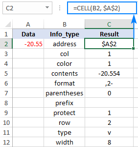
With the information you already know, you should have no difficulties with interpreting the formula results, maybe except the format type. And this leads us nicely to the next section of our tutorial.
Format codes
The below table lists the most typical values that can be returned by a CELL formula with the info_type argument set to «format».
| Format | Returned value |
| General | G |
| 0 | F0 |
| 0.00 | F2 |
| #,##0 | ,0 |
| #,##0.00 | ,2 |
| Currency with no decimal places
$#,##0 or $#,##0_);($#,##0) |
C0 |
| Currency with 2 decimal places
$#,##0.00 or $#,##0.00_);($#,##0.00) |
C2 |
| Percentage with no decimal places
0% |
P0 |
| Percentage with 2 decimal places
0.00% |
P2 |
| Scientific notation
0.00E+00 |
S2 |
| Fraction # ?/? or # ??/?? |
G |
| m/d/yy or m/d/yy h:mm or mm/dd/yy | D4 |
| d-mmm-yy or dd-mmm-yy | D1 |
| d-mmm or dd-mmm | D2 |
| mmm-yy | D3 |
| mm/dd | D5 |
| h:mm AM/PM | D7 |
| h:mm:ss AM/PM | D6 |
| h:mm | D9 |
| h:mm:ss | D8 |
For custom Excel number formats, the CELL function may return other values, and the following tips will help you to interpret them:
- The letter is usually the first letter in the format name, e.g. «G» stands for «General «, «C» for «Currency», «P» for «Percentage», «S» for «Scientific «, and «D» for «Date».
- With numbers, currencies and percentages, the digit indicates the number of displayed decimal places. For example, if the custom number format displays 3 decimal places, like 0.###, the CELL function returns «F3».
- Comma (,) is added to the beginning of the returned value if a number format has a thousands separator. For instance, for the format #,###.#### a CELL formula returns «,4» indicating that the cell is formatted as a number with 4 decimal places and a thousands separator.
- Minus sign (-) is added to the end of the returned value if the cell is formatted in color for negative values.
- Parentheses () is added to the end of the returned value if the cell is formatted with parentheses for positive or all values.
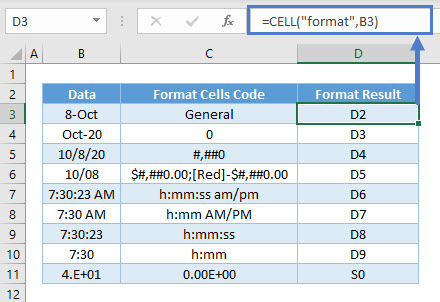
To gain more understanding of the format codes, please take a look at the results of the following formula, which is copied across column D:
=CELL(«format»,B3) 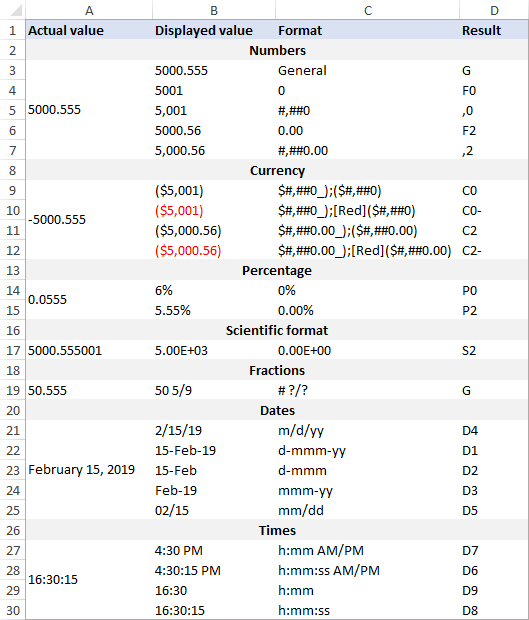
Note. If you later apply a different format to the referenced cell, you must recalculate the worksheet to update the result of a CELL formula. To recalculate the active worksheet, press Shift + F9 or use any other method described in How to recalculate Excel worksheets.
How to use the CELL function in Excel — formula examples
With the inbuilt info_types, the CELL function can return total 12 different parameters about a cell. In combination with other Excel functions, it is capable of much more. The following examples demonstrate some of the advanced capabilities.
Get address of the lookup result
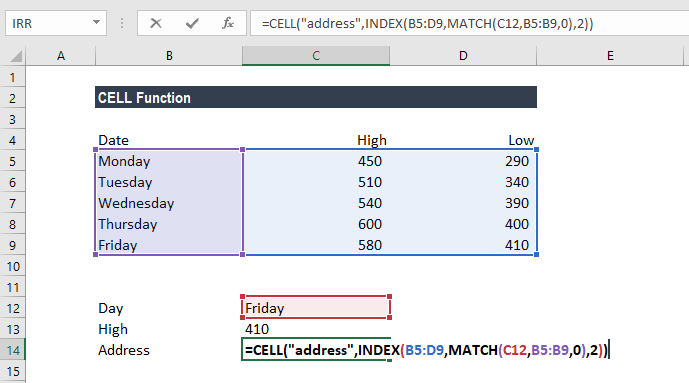
To look up a certain value in one column and return a matching value from another column, you usually use the VLOOKUP function or a more powerful INDEX MATCH combination. In case you also want to know the address of the returned value, put the Index/Match formula in the reference argument of CELL like shown below:
With the lookup value in E2, lookup range A2:A7, and return range B2:B7, the real formula goes as follows:
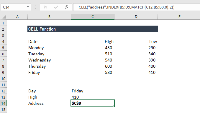
=CELL(«address», INDEX(B2:B7, MATCH(E1,A2:A7,0)))
And returns the absolute cell reference of the lookup result: 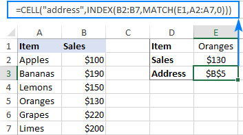
Please note that embedding the VLOOKUP function won’t work because it returns a cell value, not a reference. The INDEX function also normally displays a cell value, but it returns a cell reference underneath, which the CELL function is able to understand and process.
Make a hyperlink to the lookup result (first match)
If you wish not only to get the address of the first match, but also to jump to that match, create a hyperlink to the lookup result by using this generic formula:
In this formula, we again use the classic Index/Match combination to get the first matching value and the CELL function to extract its address. Then, we concatenate the address with the «#» character to tell HYPERLINK that the target cell is in the current sheet.
For our sample dataset, we use the same Index/Match formula as in the previous example and only need to add the desired link name, for example, this one:
=HYPERLINK(«#»&CELL(«address», INDEX(B2:B7, MATCH(E1,A2:A7,0))), «Go to lookup result») 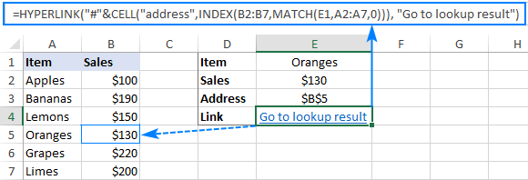
Instead to creating a hyperlink in a separate cell, you can actually turn the address into a clickable link. For this, embed the same CELL(«address», INDEX(…,MATCH()) formula into the last argument of HYPERLINK:
=HYPERLINK(«#»&CELL(«address», INDEX(B2:B7, MATCH(E1,A2:A7,0))), CELL(«address», INDEX(B2:B7, MATCH(E1,A2:A7,0))))
And make sure this lengthy formula produces a laconic and explicit result: 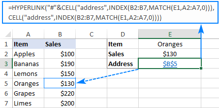
Get different parts of the file path
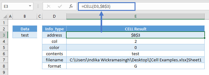
To return a full path to the workbook that contains a referenced cell, use a simple Excel CELL formula with «filename» in the info_type argument:
This will return the file path in this format: Drive:path[workbook.xlsx]sheet
To return only a specific part of the path, use the SEARCH function to determine the starting position and one of the Text functions such as LEFT, RIGHT and MID to extract the required part.
Note. All of the below formulas return the address of the current workbook and worksheet, i.e. the sheet where the formula is located.
Workbook name
To output just the file name, use the following formula:
=MID(CELL(«filename»), SEARCH(«[«, CELL(«filename»))+1, SEARCH(«]», CELL(«filename»)) — SEARCH(«[«, CELL(«filename»))-1) 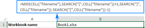
How the formula works:
The file name returned by the Excel CELL function is enclosed in square brackets, and you use the MID function to extract it.
The starting point is the position of the opening square bracket plus 1: SEARCH («[«,CELL(«filename»))+1.
The number of characters to extract corresponds to the number of characters between the opening and closing brackets, which is calculated with this formula: SEARCH(«]», CELL(«filename»)) — SEARCH(«[«, CELL(«filename»))-1
Worksheet name
To return the sheet name, use one of the following formulas:
=RIGHT(CELL(«filename»), LEN(CELL(«filename»)) — SEARCH(«]», CELL(«filename»)))
=MID(CELL(«filename»), SEARCH(«]», CELL(«filename»))+1, 31) 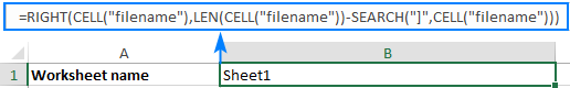
How the formulas work:
Formula 1: Working from the inside out, we calculate the number of characters in the worksheet name by subtracting the position of the closing bracket returned by SEARCH from the total path length calculated with LEN. Then, we feed this number to the RIGHT function instructing it to pull that many characters from the end of the text string returned by CELL.
Formula 2: We use the MID function to extract just the sheet name beginning with the first character after the closing bracket. The number of characters to extract is supplied as 31, which is the maximum number of characters in worksheet names allowed by the Excel UI (though Excel’s xlsx file format permits up to 255 characters in sheet names).
Path to the file
This formula will bring you the file path without the workbook and sheet names:
=LEFT(CELL(«filename»), SEARCH(«[«, CELL(«filename»))-1) 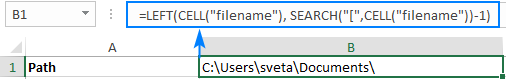
How the formula works:
First, you locate the position of the opening square bracket «[» with the SEARCH function and subtract 1. This gives you the number of characters to extract. And then, you use the LEFT function to pull that many characters from the beginning of the text string returned by CELL.
Path and file name
With this formula, you can get a full path to the file including the workbook name, but without the sheet name:
=SUBSTITUTE(LEFT(CELL(«filename»), SEARCH(«]», CELL(«filename»))-1), «[«, «») 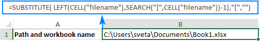
How the formula works:
The SEARCH function calculates the position of the closing square bracket, from which you subtract 1, and then get the LEFT function to extract that many characters from the beginning of the text string returned by CELL. This effectively cuts off the sheet name, but the opening square bracket remains. To get rid of it, you substitute «[» with an empty string («»).
That’s how you use the CELL function in Excel. To have a closer look at the formulas discussed in this tutorial, I invite you to download our sample Workbook below. Thank you for reading and hope to see you on our blog next week!
Источник
Get information about a cell
What is the CELL Function?
The CELL Function[1] is an Excel Information function that will extract information about a cell’s location, contents, or formatting. The CELL function takes two arguments, one that determines the type of information to be extracted and the other that is which cell it will be checking.
As a financial analyst, the CELL function is useful as it can help verify if a cell contains a numeric value instead of text before we perform a calculation on it. If we import data from an external source, we can verify that all cells with numbers are used for calculations.
Formula
=CELL(info_type, [reference])
The CELL function uses the following arguments:
- Info_type (required argument) – This is a text value specifying the type of cell information that we want to return. It can either be of the following:
| Info_type | Description |
|---|---|
| Address | It will return the address of the first cell in a reference as text. |
| Col | It will return the column number of the first cell in a reference. |
| Color | It will return the value 1 if the first cell in a reference is formatted using color for negative values, or zero if not. |
| Contents | It will return the value of the upper-left cell in a reference. Formulas are not returned. Instead, the result of the formula is returned. |
| Filename | It will return the file name and full path as text. If the worksheet that contains reference has not yet been saved, an empty string is returned. |
| Format | It will return a code that corresponds to the number format of the cell. |
| Parentheses | It will return 1 if the first cell in the reference is formatted with parentheses and 0 if not. |
| Prefix | It will return a text value corresponding to the ‘label prefix’ of the cell. |
| Protect | It will return 1 if the cell is locked, otherwise, 0. |
| Row | It will return the row number of a cell. |
| Type | It will return a text value corresponding to the type of data in the cell. It can either be «b» for blank (or empty); «l» for label (i.e. text constant), or «v» for value (for any other data type). |
| Width | It will return the column’s width. |
For the info_type format, the number format codes are as shown below:
| Format code returned | Format code meaning |
|---|---|
| G | General |
| F0 | 0 |
| ,0 | #,##0 |
| F2 | 0 |
| ,2 | #,##0.00 |
| C0 | $#,##0_);($#,##0) |
| C0- | $#,##0_);[Red]($#,##0) |
| C2 | $#,##0.00_);($#,##0.00) |
| C2- | $#,##0.00_);[Red]($#,##0.00) |
| P0 | 0% |
| P2 | 0.00% |
| S2 | 0.00E+00 |
| G | # ?/? or # ??/?? |
| D1 | d-mmm-yy or dd-mmm-yy |
| D2 | d-mmm or dd-mmm |
| D3 | mmm-yy |
| D4 | m/d/yy or m/d/yy h:mm or mm/dd/yy |
| D5 | Mm/dd |
| D6 | h:mm:ss AM/PM |
| D7 | h:mm AM/PM |
| D8 | h:mm:ss |
- Reference (optional argument) – This is the cell with the information to be returned for.
- If a range of cells is supplied, the returned information relates to the top left cell of the range.
- If the reference is omitted, the returned information relates to the last cell that was changed.
How to use the CELL function in Excel?
To understand the uses of the CELL function, let’s consider a few examples:
Example – Finding a certain value
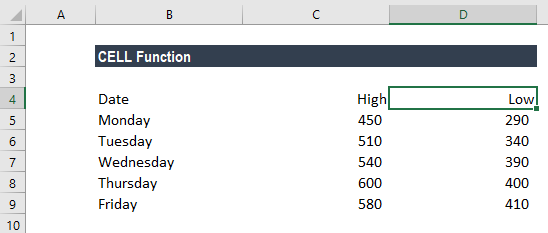
Suppose we are given the following data on stock price highs and lows. To get the address of a lookup result obtained with the INDEX function, we can use the CELL function.
The formula to use will be:
The INDEX function will display the value of a cell at a given index, but the function underneath it actually returns a reference. So, by wrapping INDEX into the ADDRESS function, we can see the address of the cell returned by the lookup.
We get the result below:
Things to remember
- #VALUE! error – Occurs when the given info_type argument is not one of the recognized types.
- The given index_num is less than 1 or is greater than the given number of values.
- The given index_num argument is non-numeric.
- #NAME? error – Occurs when the value arguments are text values that are not enclosed in quotes and are not valid cell references.
Click here to download the sample Excel file
Additional Resources
Thanks for reading CFI’s guide to important Excel functions! By taking the time to learn and master these functions, you’ll significantly speed up your financial analysis. To learn more, check out these additional CFI resources:
- Excel Functions for Finance
- Advanced Excel Formulas Course
- Advanced Excel Formulas You Must Know
- Compare Finance Certifications
- See all Excel resources
Article Sources
- CELL Function
Use the CELL function to return a wide range of information about a reference. The type of information returned is given as info_type, which must be enclosed in double quotes («»). CELL can return a cell’s address, the filename and path for a workbook, and information about the formatting used in the cell. See below for a full list of info types and format codes.
CELL is a volatile function, and can cause performance issues in large or complex worksheets.
The CELL function takes two arguments: info_type and reference. Info_type is a text string that indicates the type of information requested. See the table below for a full list of info types. Reference is a cell reference. Reference is typically a single cell. If reference refers to more than one cell, CELL returns information about the first cell in reference. For certain kinds of information (like filename) the cell address used for reference is optional and can be omitted. However, if reference is not supplied, CELL will return the name of the current «active sheet» which may or may not be the sheet where the formula exists, and might even be in a different workbook. To avoid confusion, use A1 for reference.
Note: the CELL function is a volatile function and may cause performance issues in large or complex worksheets.
Examples
For example, to get the column number for C10:
=CELL("col", C10) // returns 3
To get the address of A1 as text:
=CELL("address",A1) // returns "$A$1"
To get the full path and workbook name for the current worksheet:
=CELL("filename",A1) // path + filename
CELL can also return format code information. For example, if A1 contains the number 100 with the currency number format applied, the CELL function will return «C2»:
=CELL("format",A1) // returns "C2"
When requesting the info_type «format» or «parentheses», a set of empty parentheses «()» is appended to the format returned if the number format uses parentheses for all values or for positive values. For example, if A1 uses the custom number format (0), then:
=CELL("format",A1) // returns "F0()"
Info types
The following info_types can be used with the CELL function:
| Info_type | Description |
|---|---|
| address | returns the address of the first cell in reference (as text). |
| col | returns the column number of the first cell in reference. |
| color | returns the value 1 if the first cell in reference is formatted using color for negative values; or zero if not. |
| contents | returns the value of the upper-left cell in reference. Formulas are not returned. Instead, the result of the formula is returned. |
| filename | returns the file name and full path as text. If the worksheet that contains reference has not yet been saved, an empty string is returned. |
| format | returns a code that corresponds to the number format of the cell. See below for a list of number format codes. If the first cell in reference is formatted with color for values < 0, then «-» is appended to the code. If the cell is formatted with parentheses, returns «() — at the end of the code value. |
| parentheses | returns 1 if the first cell in reference is formatted with parentheses and 0 if not. |
| prefix | returns a text value that corresponds to the label prefix — of the cell: a single quotation mark (‘) if the cell text is left-aligned, a double quotation mark («) if the cell text is right-aligned, a caret (^) if the cell text is centered text, a backslash () if the cell text is fill-aligned, and an empty string if the label prefix is anything else. |
| protect | returns 1 if the first cell in reference is locked or 0 if not. |
| row | returns the row number of the first cell in reference. |
| type | returns a text value that corresponds to the type of data in the first cell in reference: «b» for blank when the cell is empty, «l» for label if the cell contains a text constant, and «v» for value if the cell contains anything else. |
| width | returns the column width of the cell, rounded to the nearest integer. A unit of column width is equal to the width of one character in the default font size. Note: this value comes back as an array with two values {width,default} where width is the column width and default is a boolean value that indicates if the width is the default column width. |
Format codes
The table below shows the text codes returned by CELL when «format» is used for info_type.
| Format code returned | Format code meaning |
|---|---|
| G | General |
| F0 | 0 |
| ,0 | #,##0 |
| F2 | 0 |
| ,2 | #,##0.00 |
| C0 | $#,##0_);($#,##0) |
| C0- | $#,##0_);[Red]($#,##0) |
| C2 | $#,##0.00_);($#,##0.00) |
| C2- | $#,##0.00_);[Red]($#,##0.00) |
| P0 | 0% |
| P2 | 0.00% |
| S2 | 0.00E+00 |
| G | # ?/? or # ??/?? |
| D1 | d-mmm-yy or dd-mmm-yy |
| D2 | d-mmm or dd-mmm |
| D3 | mmm-yy |
| D4 | m/d/yy or m/d/yy h:mm or mm/dd/yy |
| D5 | mm/dd |
| D6 | h:mm:ss AM/PM |
| D7 | h:mm AM/PM |
| D8 | h:mm:ss |
Notes
- The CELL function is a volatile function and may cause performance issues in large or complex worksheets.
- Reference is optional for some info types, but use an address like A1 to avoid unexpected behavior.
Very often, when working in Excel, you need to use data about addressing cells in a spreadsheet. For this was provided the function CELL. Consider its use on specific examples.
Function CELL value and properties in Excel
It should be noted that Excel uses several functions for addressing cells:
- — ROW;
- — COLUMN and others.
CELL function return information about the formatting, address, or contents of a cell. The function can return detailed information about the cell format, thereby eliminating the need to use VBA in some cases. The function is especially useful if you need to display the full path of the file in the cells.
How does the CELL function in Excel work?
Function in its work uses the syntax that consists of two arguments:
=CELL(info_type,[reference])
- Info_type is a text value that specifies the type of cell information that is required. When you enter a function manually, a drop-down list is displayed where all possible values of the “information type” argument are shown:
- [Reference] is an optional argument. The cell for which you want to receive information. If this argument is omitted, the information specified in the information_type argument is returned for the last cell changed. If the link argument points to a range of cells, function returns information only for the upper-left value of the range.
Examples of using the CELL function in Excel
Example 1. Given the table of accounting work of employees of the organization of the form:
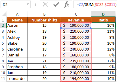
It is necessary with the help of the CELL function to calculate in which row and column the salary is in the amount of 235,000 dollars.
To do this, we introduce the following formula:
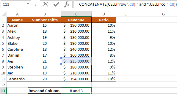
here:
- — «row» and «column» — output parameter;
- — C8 — address data with a salary.
As a result of the calculations, we obtain: row №8 and column № 3 (C).
How to know width of an Excel spreadsheet?
Example 2. It is necessary to calculate the width of the table in characters. Immediately it should be noted that in Excel, by default, the width of columns and cells is measured in the number of characters that they fit in their value are available for display in a cell without a line break.
Note. The height of lines and cells in Excel is by default measured in units of the basic font — in (pt) points. The larger the font, the higher the line for full display of characters in height.
Let’s enter into C14 the formula for calculating the sum of the width of each column of the table:
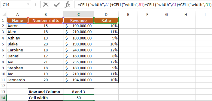
here:
- — «width» is a function parameter;
- — A1 — the width of a specific column.
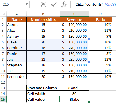
How to get the value of the first value in the range
Example 3. In the condition of example 1, you need to display the contents of only the first (upper left) value from the range A5:C8.
We introduce the formula for calculating:
Download examples CELL function in Excel
Description of the formula is similar to the previous two examples.