
Содержание
- Select cell contents in Excel
- Select one or more cells
- Select one or more rows and columns
- Select table, list or worksheet
- Need more help?
- What Can A Cell Contain In Excel?
- What are cell in Excel?
- Can a cell only contain a number in Excel?
- What is a cell?
- What are the basics of cell?
- What is cell content?
- How can I tell if a cell contains numbers?
- How do you check if a cell contains only alphabets in Excel?
- What is cell and its components?
- What is cell and its organelles?
- What does it mean to be made of cells?
- What is a typical cell?
- What are the five main functions of a cell?
- What are the 3 basic types of cells?
- How many characters can a cell contain?
- Where is cell in Excel?
- How do I identify a cell in Excel?
- Is Google sheet a number?
- What is Excel VLOOKUP?
- How does a VLOOKUP work?
- How do I identify alphabets in Excel?
- Excel —
- Cell Basics
- Excel: Cell Basics
- Lesson 5: Cell Basics
- Introduction
- Understanding cells
- To select a cell:
- To select a cell range:
- Cell content
- To insert content:
- To delete (or clear) cell content:
- To delete cells:
- To copy and paste cell content:
- To access additional paste options:
- To cut and paste cell content:
- To drag and drop cells:
- To use the fill handle:
- To continue a series with the fill handle:
Select cell contents in Excel
In Excel, you can select cell contents of one or more cells, rows and columns.

Note: If a worksheet has been protected, you might not be able to select cells or their contents on a worksheet.
Select one or more cells
Click on a cell to select it. Or use the keyboard to navigate to it and select it.
To select a range, select a cell, then with the left mouse button pressed, drag over the other cells.
Or use the Shift + arrow keys to select the range.
To select non-adjacent cells and cell ranges, hold Ctrl and select the cells.
Select one or more rows and columns
Select the letter at the top to select the entire column. Or click on any cell in the column and then press Ctrl + Space.
Select the row number to select the entire row. Or click on any cell in the row and then press Shift + Space.
To select non-adjacent rows or columns, hold Ctrl and select the row or column numbers.
Select table, list or worksheet
To select a list or table, select a cell in the list or table and press Ctrl + A.
To select the entire worksheet, click the Select All button at the top left corner.

Note: In some cases, selecting a cell may result in the selection of multiple adjacent cells as well. For tips on how to resolve this issue, see this post How do I stop Excel from highlighting two cells at once? in the community.
Click the cell, or press the arrow keys to move to the cell.
A range of cells
Click the first cell in the range, and then drag to the last cell, or hold down SHIFT while you press the arrow keys to extend the selection.
You can also select the first cell in the range, and then press F8 to extend the selection by using the arrow keys. To stop extending the selection, press F8 again.
A large range of cells
Click the first cell in the range, and then hold down SHIFT while you click the last cell in the range. You can scroll to make the last cell visible.
All cells on a worksheet
Click the Select All button.
To select the entire worksheet, you can also press CTRL+A.
Note: If the worksheet contains data, CTRL+A selects the current region. Pressing CTRL+A a second time selects the entire worksheet.
Nonadjacent cells or cell ranges
Select the first cell or range of cells, and then hold down CTRL while you select the other cells or ranges.
You can also select the first cell or range of cells, and then press SHIFT+F8 to add another nonadjacent cell or range to the selection. To stop adding cells or ranges to the selection, press SHIFT+F8 again.
Note: You cannot cancel the selection of a cell or range of cells in a nonadjacent selection without canceling the entire selection.
An entire row or column
Click the row or column heading.
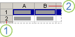
2. Column heading
You can also select cells in a row or column by selecting the first cell and then pressing CTRL+SHIFT+ARROW key (RIGHT ARROW or LEFT ARROW for rows, UP ARROW or DOWN ARROW for columns).
Note: If the row or column contains data, CTRL+SHIFT+ARROW key selects the row or column to the last used cell. Pressing CTRL+SHIFT+ARROW key a second time selects the entire row or column.
Adjacent rows or columns
Drag across the row or column headings. Or select the first row or column; then hold down SHIFT while you select the last row or column.
Nonadjacent rows or columns
Click the column or row heading of the first row or column in your selection; then hold down CTRL while you click the column or row headings of other rows or columns that you want to add to the selection.
The first or last cell in a row or column
Select a cell in the row or column, and then press CTRL+ARROW key (RIGHT ARROW or LEFT ARROW for rows, UP ARROW or DOWN ARROW for columns).
The first or last cell on a worksheet or in a Microsoft Office Excel table
Press CTRL+HOME to select the first cell on the worksheet or in an Excel list.
Press CTRL+END to select the last cell on the worksheet or in an Excel list that contains data or formatting.
Cells to the last used cell on the worksheet (lower-right corner)
Select the first cell, and then press CTRL+SHIFT+END to extend the selection of cells to the last used cell on the worksheet (lower-right corner).
Cells to the beginning of the worksheet
Select the first cell, and then press CTRL+SHIFT+HOME to extend the selection of cells to the beginning of the worksheet.
More or fewer cells than the active selection
Hold down SHIFT while you click the last cell that you want to include in the new selection. The rectangular range between the active cell and the cell that you click becomes the new selection.
Need more help?
You can always ask an expert in the Excel Tech Community or get support in the Answers community.
Источник
What Can A Cell Contain In Excel?
Each cell can contain different types of content, including text, formatting, formulas, and functions. Cells can contain text, such as letters, numbers, and dates. Cells can contain formatting attributes that change the way letters, numbers, and dates are displayed. For example, percentages can appear as 0.15 or 15%.
What are cell in Excel?
Cells are the boxes you see in the grid of an Excel worksheet, like this one. Each cell is identified on a worksheet by its reference, the column letter and row number that intersect at the cell’s location. This cell is in column D and row 5, so it is cell D5. The column always comes first in a cell reference.
Can a cell only contain a number in Excel?
Note: Excel has several built-in data validation rules for numbers. This page explains how to create a your own validation rule based on a custom formula. To allow only numbers in a cell, you can use data validation with a custom formula based on the ISNUMBER function.
What is a cell?
In biology, the smallest unit that can live on its own and that makes up all living organisms and the tissues of the body. A cell has three main parts: the cell membrane, the nucleus, and the cytoplasm.Parts of a cell. A cell is surrounded by a membrane, which has receptors on the surface.
What are the basics of cell?
Cells are the basic building blocks of all living things. The human body is composed of trillions of cells. They provide structure for the body, take in nutrients from food, convert those nutrients into energy, and carry out specialized functions.
What is cell content?
Cell content. Any information you enter into a spreadsheet will be stored in a cell. Each cell can contain different types of content, including text, formatting, formulas, and functions. Text. Cells can contain text, such as letters, numbers, and dates.
How can I tell if a cell contains numbers?
To test if a cell (or any text string) contains a number, you can use the FIND function together with the COUNT function. In the generic form of the formula (above), A1 represents the cell you are testing. The numbers to be checked (numbers between 0-9) are supplied as an array.
How do you check if a cell contains only alphabets in Excel?
You’ll need to open your Excel spreadsheet. Press Alt + F11 and create a new module. The AlphaNumeric function will return TRUE if all of the values in the string are alphanumeric. Otherwise, it will return FALSE.
What is cell and its components?
A cell consists of three parts: the cell membrane, the nucleus, and, between the two, the cytoplasm. Within the cytoplasm lie intricate arrangements of fine fibers and hundreds or even thousands of miniscule but distinct structures called organelles.
What is cell and its organelles?
An organelle is a subcellular structure that has one or more specific jobs to perform in the cell, much like an organ does in the body. Among the more important cell organelles are the nuclei, which store genetic information; mitochondria, which produce chemical energy; and ribosomes, which assemble proteins.
What does it mean to be made of cells?
The first characteristic of a living thing is that they are made up of cells. A cell is the basic building block of all organisms. It is the smallest unit of organization in a living thing. They contain the organism’s hereditary information (DNA) and can make copies of themselves in a process called mitosis.
What is a typical cell?
Answer: A typical cell is a generalized cell diagram which represents all the different cell organelles that exist in an animal cell or a plant cell.
What are the five main functions of a cell?
They provide structure and support, facilitate growth through mitosis, allow passive and active transport, produce energy, create metabolic reactions and aid in reproduction.
What are the 3 basic types of cells?
Basic Types of Cells
- Epithelial Cells. These cells are tightly attached to one another.
- Nerve Cells. These cells are specialized for communication.
- Muscle Cells. These cells are specialized for contraction.
- Connective Tissue Cells.
How many characters can a cell contain?
Total number of characters that a cell can contain 32,767 characters.
Where is cell in Excel?
In Microsoft Excel, a cell is a rectangular box that occurs at the intersection of a vertical column and a horizontal row in a worksheet.
How do I identify a cell in Excel?
Go to the Formulas tab and select More Functions > Information > TYPE. Select a cell in the worksheet to enter the cell reference. Select OK to complete the function.
Is Google sheet a number?
The ISNUMBER function is fairly simple. It checks if a value is a number and returns a corresponding Boolean value. If the value is a number, the function returns TRUE. if not, it returns FALSE.
What is Excel VLOOKUP?
VLOOKUP stands for ‘Vertical Lookup’. It is a function that makes Excel search for a certain value in a column (the so called ‘table array’), in order to return a value from a different column in the same row.
How does a VLOOKUP work?
The VLOOKUP function performs a vertical lookup by searching for a value in the first column of a table and returning the value in the same row in the index_number position. The VLOOKUP function is a built-in function in Excel that is categorized as a Lookup/Reference Function.
How do I identify alphabets in Excel?
To use the function, enter =LEN(cell) in the formula bar and press Enter. In these examples, cell is the cell you want to count, such as B1. To count the characters in more than one cell, enter the formula, and then copy and paste the formula to other cells.
Источник
Excel —
Cell Basics


Excel: Cell Basics
Lesson 5: Cell Basics
Introduction
Whenever you work with Excel, you’ll enter information—or content—into cells. Cells are the basic building blocks of a worksheet. You’ll need to learn the basics of cells and cell content to calculate, analyze, and organize data in Excel.
Watch the video below to learn more about the basics of working with cells.
Understanding cells
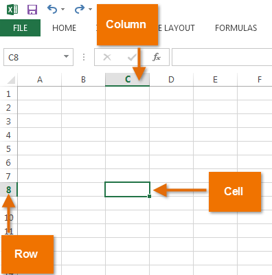
Every worksheet is made up of thousands of rectangles, which are called cells. A cell is the intersection of a row and a column. In other words, it’s where a row and column meet.
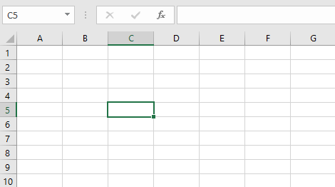
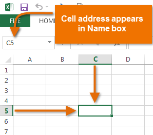
Columns are identified by letters (A, B, C), while rows are identified by numbers (1, 2, 3). Each cell has its own name—or cell address—based on its column and row. In the example below, the selected cell intersects column C and row 5, so the cell address is C5.
Note that the cell address also appears in the Name box in the top-left corner, and that a cell’s column and row headings are highlighted when the cell is selected.
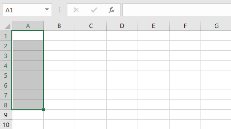
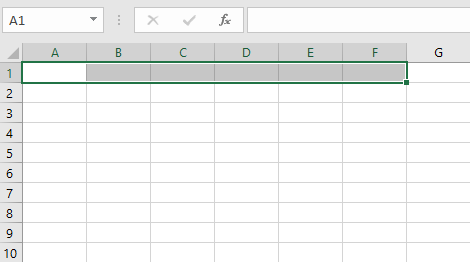
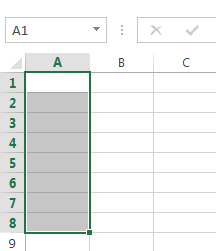
You can also select multiple cells at the same time. A group of cells is known as a cell range. Rather than a single cell address, you will refer to a cell range using the cell addresses of the first and last cells in the cell range, separated by a colon. For example, a cell range that included cells A1, A2, A3, A4, and A5 would be written as A1:A5. Take a look at the different cell ranges below:
- Cell range A1:A8
Cell range A1:F1
If the columns in your spreadsheet are labeled with numbers instead of letters, you’ll need to change the default reference style for Excel. Review our Extra on What are Reference Styles? to learn how.
To select a cell:
To input or edit cell content, you’ll first need to select the cell.
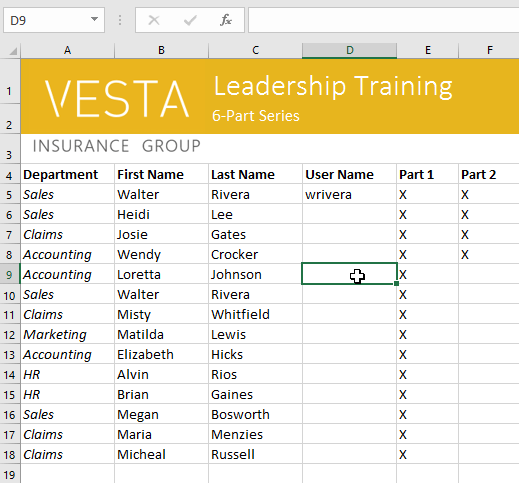
- Click a cell to select it. In our example, we’ll select cell D9.
- A border will appear around the selected cell, and the column heading and row heading will be highlighted. The cell will remain selected until you click another cell in the worksheet.
You can also select cells using the arrow keys on your keyboard.
To select a cell range:
Sometimes you may want to select a larger group of cells, or a cell range.
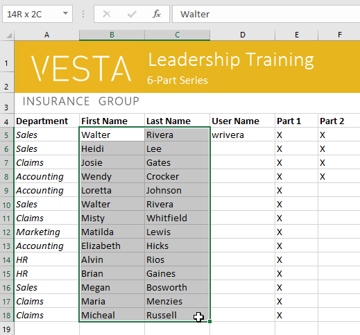
- Click and drag the mouse until all of the adjoiningcells you want to select are highlighted. In our example, we’ll select the cell range B5:C18.
- Release the mouse to select the desired cell range. The cells will remain selected until you click another cell in the worksheet.
Cell content
Any information you enter into a spreadsheet will be stored in a cell. Each cell can contain different types of content, including text, formatting, formulas, and functions.
- Text: Cells can contain text, such as letters, numbers, and dates.
To insert content:
- Click a cell to select it. In our example, we’ll select cell F9.
To delete (or clear) cell content:
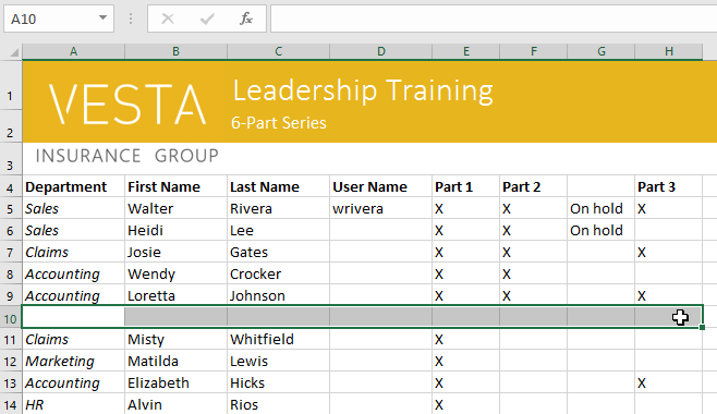
- Select the cell(s) with content you want to delete. In our example, we’ll select the cell range A10:H10.
![]()
![]()
![]()
You can also use the Delete key on your keyboard to delete content from multiple cells at once. The Backspace key will only delete content from one cell at a time.
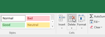
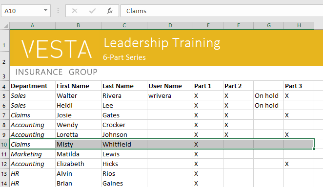
To delete cells:
There is an important difference between deleting the content of a cell and deleting the cell itself. If you delete the entire cell, the cells below it will shift to fill in the gaps and replace the deleted cells.
- Select the cell(s) you want to delete. In our example, we’ll select A10:H10.
Select the Delete command from the Home tab on the Ribbon.
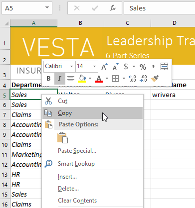
To copy and paste cell content:
Excel allows you to copy content that is already entered into your spreadsheet and paste this content to other cells, which can save you time and effort.
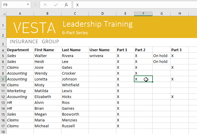
- Select the cell(s) you want to copy. In our example, we’ll select F9.
To access additional paste options:
You can also access additional paste options, which are especially convenient when working with cells that contain formulas or formatting. Just click the drop-down arrow on the Paste command to see these options.
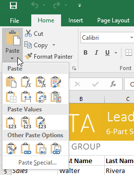
Instead of choosing commands from the Ribbon, you can access commands quickly by right-clicking. Simply select the cell(s) you want to format, then right-click the mouse. A drop-down menu will appear, where you’ll find several commands that are also located on the Ribbon.
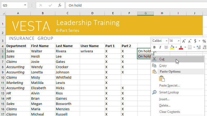
To cut and paste cell content:
Unlike copying and pasting, which duplicates cell content, cutting allows you to move content between cells.
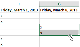
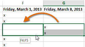
- Select the cell(s) you want to cut. In our example, we’ll select G5:G6.
- Right-click the mouse and select the Cut command. You can also use the command on the Home tab, or press Ctrl+X on your keyboard.
To drag and drop cells:
Instead of cutting, copying, and pasting, you can drag and drop cells to move their contents.
- Select the cell(s) you want to move. In our example, we’ll select H4:H12.
- Hover the mouse over the border of the selected cell(s) until the mouse changes to a pointer with four arrows.
To use the fill handle:
If you’re copying cell content to adjacent cells in the same row or column, the fill handle is a good alternative to the copy and paste commands.
- Select the cell(s) containing the content you want to use, then hover the mouse over the lower-right corner of the cell so the fill handle appears.
To continue a series with the fill handle:
The fill handle can also be used to continue a series. Whenever the content of a row or column follows a sequential order, like numbers (1, 2, 3) or days (Monday, Tuesday, Wednesday), the fill handle can guess what should come next in the series. In most cases, you will need to select multiple cells before using the fill handle to help Excel determine the series order. Let’s take a look at an example:
- Select the cell range that contains the series you want to continue. In our example, we’ll select E4:G4.
- Click and drag the fill handle to continue the series.
You can also double-click the fill handle instead of clicking and dragging. This can be useful with larger spreadsheets, where clicking and dragging may be awkward.
Watch the video below to see an example of double-clicking the fill handle.
Источник
![]()
What is Contents in Excel?

The information or Objects used in Excel Workbooks to visualize the data is called Contents in Excel. All the Objects in a Workbook or information stored in an Excel Object are Contents in Excel. For example: Excel Charts and Shapes are the contents in the Excel Sheets. We can able to visualize the data using these Container or Objects in Excel. Excel Cells contests are the text or any data entered in a Cell is called Cell Contents.
Excel Cell Contents:
All the information entered or stored in a Cell is called Cell Contents. We perform verity of operations using Cell contents. For example, we can refer the content from another Cell, or from another sheet. We can refer the Cell content from one sheet to another sheet. We can put the cell contents in a Shape or Chart Titles.
Clear Contents Command:
Excel is provided with ready to use command to Clear the Cell Contents. We can use this command to clear only the content of the Selected Cells and remain the formatting and comments as it is. Follow the below steps to execute the Clear Contents commands
- Select the Cell
- Go to Home Tab
- Click on Clear commands (this will display the List of Commands to Clear)
- Click on the Clear Contents to Clear the Cell Contents
Similarly, you can select Charts, Shapes in the Excel Sheets to Clear it.
Using the Excel Functions to Deal with Cell Contents:
The following formula can be used in Excel to deal with Cell Contents
- CONCATENATE: To combine the Cell contents from multiple cells into to one Cell
- LEN: To find the Length of Cell Contents
- TRIM: To remove the extra spaces from Cell Contents
- SUM: To find the Total of Range of Cell Contents
- COUNT: To Count the number of Cells with Cell Contents
Share This Story, Choose Your Platform!
© Copyright 2012 – 2020 | Excelx.com | All Rights Reserved
Page load link
Select cell contents in Excel
In Excel, you can select cell contents of one or more cells, rows and columns.
Note: If a worksheet has been protected, you might not be able to select cells or their contents on a worksheet.
Select one or more cells
-
Click on a cell to select it. Or use the keyboard to navigate to it and select it.
-
To select a range, select a cell, then with the left mouse button pressed, drag over the other cells.
Or use the Shift + arrow keys to select the range.
-
To select non-adjacent cells and cell ranges, hold Ctrl and select the cells.
Select one or more rows and columns
-
Select the letter at the top to select the entire column. Or click on any cell in the column and then press Ctrl + Space.
-
Select the row number to select the entire row. Or click on any cell in the row and then press Shift + Space.
-
To select non-adjacent rows or columns, hold Ctrl and select the row or column numbers.
Select table, list or worksheet
-
To select a list or table, select a cell in the list or table and press Ctrl + A.
-
To select the entire worksheet, click the Select All button at the top left corner.

Note: In some cases, selecting a cell may result in the selection of multiple adjacent cells as well. For tips on how to resolve this issue, see this post How do I stop Excel from highlighting two cells at once? in the community.
|
To select |
Do this |
|---|---|
|
A single cell |
Click the cell, or press the arrow keys to move to the cell. |
|
A range of cells |
Click the first cell in the range, and then drag to the last cell, or hold down SHIFT while you press the arrow keys to extend the selection. You can also select the first cell in the range, and then press F8 to extend the selection by using the arrow keys. To stop extending the selection, press F8 again. |
|
A large range of cells |
Click the first cell in the range, and then hold down SHIFT while you click the last cell in the range. You can scroll to make the last cell visible. |
|
All cells on a worksheet |
Click the Select All button.
To select the entire worksheet, you can also press CTRL+A. Note: If the worksheet contains data, CTRL+A selects the current region. Pressing CTRL+A a second time selects the entire worksheet. |
|
Nonadjacent cells or cell ranges |
Select the first cell or range of cells, and then hold down CTRL while you select the other cells or ranges. You can also select the first cell or range of cells, and then press SHIFT+F8 to add another nonadjacent cell or range to the selection. To stop adding cells or ranges to the selection, press SHIFT+F8 again. Note: You cannot cancel the selection of a cell or range of cells in a nonadjacent selection without canceling the entire selection. |
|
An entire row or column |
Click the row or column heading.
1. Row heading 2. Column heading You can also select cells in a row or column by selecting the first cell and then pressing CTRL+SHIFT+ARROW key (RIGHT ARROW or LEFT ARROW for rows, UP ARROW or DOWN ARROW for columns). Note: If the row or column contains data, CTRL+SHIFT+ARROW key selects the row or column to the last used cell. Pressing CTRL+SHIFT+ARROW key a second time selects the entire row or column. |
|
Adjacent rows or columns |
Drag across the row or column headings. Or select the first row or column; then hold down SHIFT while you select the last row or column. |
|
Nonadjacent rows or columns |
Click the column or row heading of the first row or column in your selection; then hold down CTRL while you click the column or row headings of other rows or columns that you want to add to the selection. |
|
The first or last cell in a row or column |
Select a cell in the row or column, and then press CTRL+ARROW key (RIGHT ARROW or LEFT ARROW for rows, UP ARROW or DOWN ARROW for columns). |
|
The first or last cell on a worksheet or in a Microsoft Office Excel table |
Press CTRL+HOME to select the first cell on the worksheet or in an Excel list. Press CTRL+END to select the last cell on the worksheet or in an Excel list that contains data or formatting. |
|
Cells to the last used cell on the worksheet (lower-right corner) |
Select the first cell, and then press CTRL+SHIFT+END to extend the selection of cells to the last used cell on the worksheet (lower-right corner). |
|
Cells to the beginning of the worksheet |
Select the first cell, and then press CTRL+SHIFT+HOME to extend the selection of cells to the beginning of the worksheet. |
|
More or fewer cells than the active selection |
Hold down SHIFT while you click the last cell that you want to include in the new selection. The rectangular range between the active cell and the cell that you click becomes the new selection. |
Need more help?
You can always ask an expert in the Excel Tech Community or get support in the Answers community.
See Also
Select specific cells or ranges
Add or remove table rows and columns in an Excel table
Move or copy rows and columns
Transpose (rotate) data from rows to columns or vice versa
Freeze panes to lock rows and columns
Lock or unlock specific areas of a protected worksheet
Need more help?
Cell contents returns only the value in the cell. This is often the only thing you need, and in many formulae it would be fine to use the =X in your example (the Cell function also gives you access to a lot more information about the cell though, eg type, etc).
However indirect lets you do more, as rather than just passing the value from a cell, it creates a reference to the cell, which could then be used in formulae. Cell contents won’t let you do this.
Cell would let you do this:
A1="thing I'm looking up"
=vlookup(cell.contents("contents",A1), myRange,1,false)
or even this:
A1="B2"
B2="thing i'm looking up"
=vlookup(cell.contents("contents",indirect(A1)), myRange,1,false)
But it won’t let you do this:
A1="B3:C5"
vlookup("thing I'm looking up in " & A1, indirect(A1), 1, false)
where you could use the address stored in A1 as a reference to be used in a formula. Cell only lets you use the value, and not as a reference.
Lesson 7: Cell Basics
/en/excel2013/saving-and-sharing-workbooks/content/
Introduction
Whenever you work with Excel, you’ll enter information—or content—into cells. Cells are the basic building blocks of a worksheet. You’ll need to learn the basics of cells and cell content to calculate, analyze, and organize data in Excel.
Optional: Download our practice workbook.
Understanding cells
Every worksheet is made up of thousands of rectangles, which are called cells. A cell is the intersection of a row and a column. Columns are identified by letters (A, B, C), while rows are identified by numbers (1, 2, 3).
 A cell
Each cell has its own name—or cell address—based on its column and row. In this example, the selected cell intersects column C and row 5, so the cell address is C5. The cell address will also appear in the Name box. Note that a cell’s column and row headings are highlighted when the cell is selected.
 Cell C5
You can also select multiple cells at the same time. A group of cells is known as a cell range. Rather than a single cell address, you will refer to a cell range using the cell addresses of the first and last cells in the cell range, separated by a colon. For example, a cell range that included cells A1, A2, A3, A4, and A5 would be written as A1:A5.
In the images below, two different cell ranges are selected:
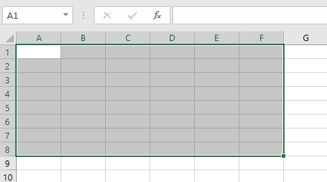
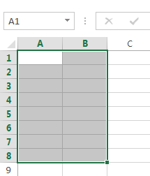
- Cell range A1:A8
Cell range A1:A8
- Cell range A1:B8
Cell range A1:B8
If the columns in your spreadsheet are labeled with numbers instead of letters, you’ll need to change the default reference style for Excel. Review our Extra on What are Reference Styles? to learn how.
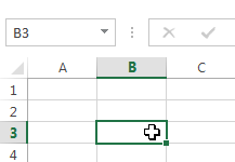
To select a cell:
To input or edit cell content, you’ll first need to select the cell.
- Click a cell to select it.
- A border will appear around the selected cell, and the column heading and row heading will be highlighted. The cell will remain selected until you click another cell in the worksheet.
 Selecting a single cell
 will appear around the selected cell, and the column heading and row heading will be highlighted. The cell will remain selected until you click another cell in the worksheet.
You can also select cells using the arrow keys on your keyboard.
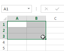
To select a cell range:
Sometimes you may want to select a larger group of cells, or a cell range.
- Click, hold, and drag the mouse until all of the adjoining cells you want to select are highlighted.
- Release the mouse to select the desired cell range. The cells will remain selected until you click another cell in the worksheet.
 Selecting a cell range
Cell content
Any information you enter into a spreadsheet will be stored in a cell. Each cell can contain different types of content, including text, formatting, formulas, and functions.
- Text
Cells can contain text, such as letters, numbers, and dates. Cell text
 - Formatting attributes
Cells can contain formatting attributes that change the way letters, numbers, and dates are displayed. For example, percentages can appear as 0.15 or 15%. You can even change a cell’s background color. Cell formatting
 - Formulas and functions
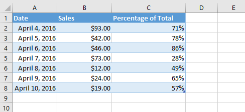
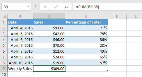
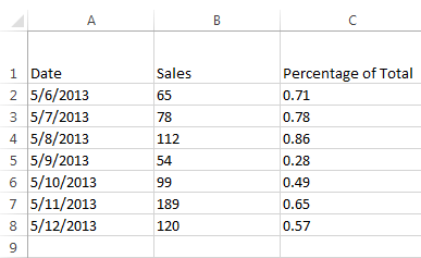
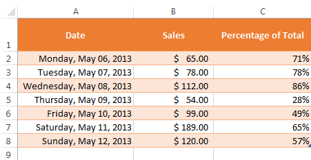
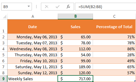
Cells can contain formulas and functions that calculate cell values. In our example, SUM(B2:B8) adds the value of each cell in cell range B2:B8 and displays the total in cell B9. Cell formulas
To insert content:
- Click a cell to select it.
 Selecting cell A1
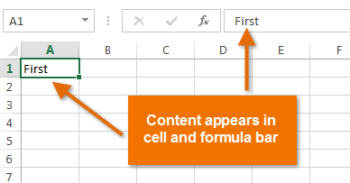
 - Type content into the selected cell, then press Enter on your keyboard. The content will appear in the cell and the formula bar. You can also input and edit cell content in the formula bar.
 Inserting cell content
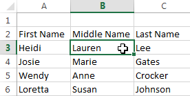
To delete cell content:
- Select the cell with content you want to delete.
 Selecting a cell
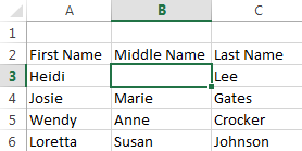
 - Press the Delete or Backspace key on your keyboard. The cell’s contents will be deleted.
 Deleting cell content
You can use the Delete key on your keyboard to delete content from multiple cells at once. The Backspace key will only delete one cell at a time.
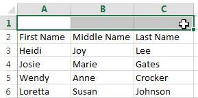
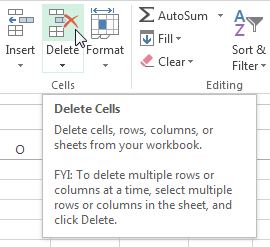
To delete cells:
There is an important difference between deleting the content of a cell and deleting the cell itself. If you delete the entire cell, the cells below it will shift up and replace the deleted cells.
- Select the cell(s) you want to delete.
 Selecting a cell to delete
 - Select the Delete command from the Home tab on the Ribbon.
 Clicking the Delete command
 - The cells below will shift up.
 Cells shifted to replace the deleted cell
To copy and paste cell content:
Excel allows you to copy content that is already entered into your spreadsheet and paste that content to other cells, which can save you time and effort.
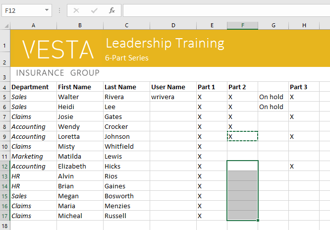
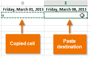
- Select the cell(s) you want to copy.
 Selecting a cell to copy
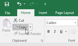
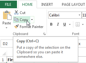
 - Click the Copy command on the Home tab, or press Ctrl+C on your keyboard.
 Clicking the Copy command
 - Select the cell(s) where you want to paste the content. The copied cells will now have a dashed box around them.
 Pasting cells
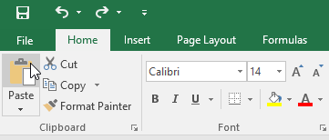
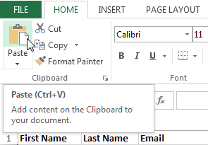
 - Click the Paste command on the Home tab, or press Ctrl+V on your keyboard.
 Clicking the Paste command
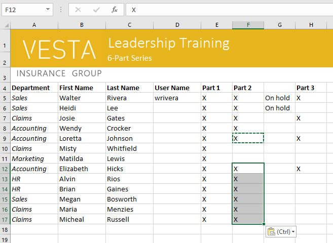
 - The content will be pasted into the selected cells.
 The pasted cell content
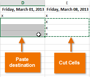
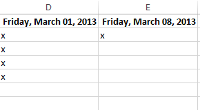
To cut and paste cell content:
Unlike copying and pasting, which duplicates cell content, cutting allows you to move content between cells.
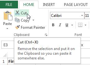
- Select the cell(s) you want to cut.
 Selecting a cell range to cut
 - Click the Cut command on the Home tab, or press Ctrl+X on your keyboard.
 Clicking the Cut command
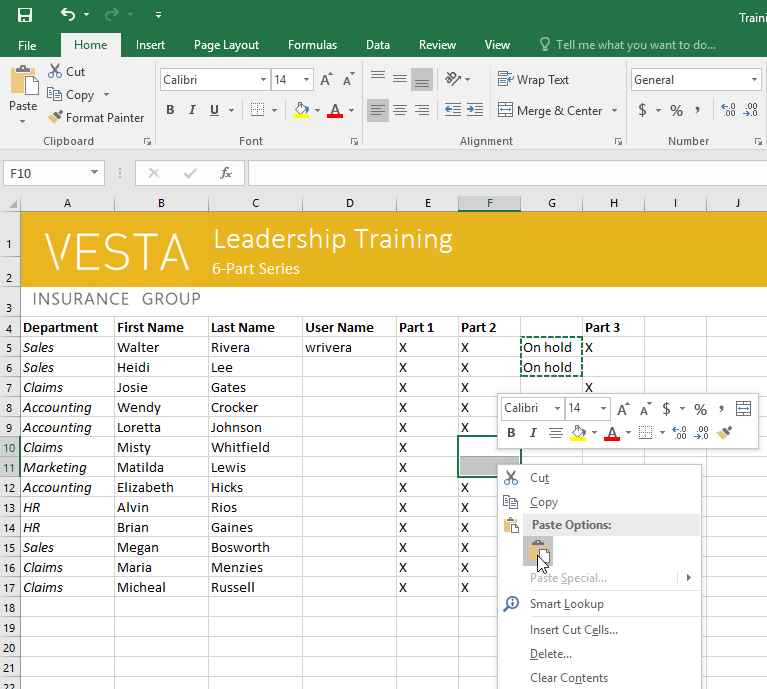
 - Select the cells where you want to paste the content. The cut cells will now have a dashed box around them.
 Pasting cells
 - Click the Paste command on the Home tab, or press Ctrl+V on your keyboard.
Clicking the Paste command
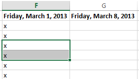
- The cut content will be removed from the original cells and pasted into the selected cells.
 The cut and pasted cells
To access more paste options:
You can also access additional paste options, which are especially convenient when working with cells that contain formulas or formatting.
- To access more paste options, click the drop-down arrow on the Paste command.
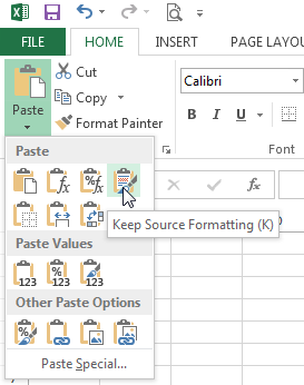 Additional Paste options
Rather than choose commands from the Ribbon, you can access commands quickly by right-clicking. Simply select the cell(s) you want to format, then right-click the mouse. A drop-down menu will appear, where you’ll find several commands that are also located on the Ribbon.
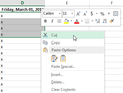 Right-clicking to access formatting options
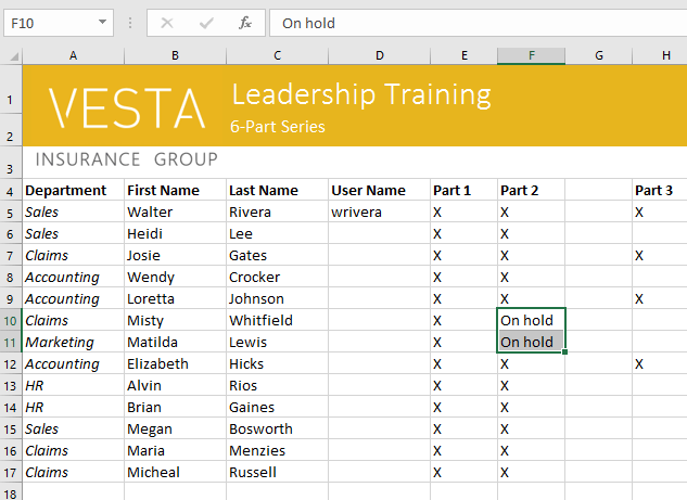
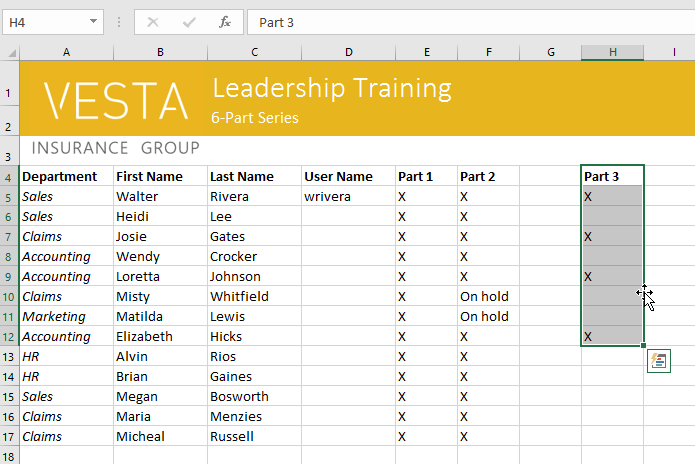
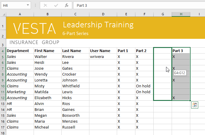
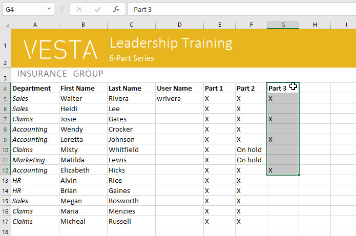
To drag and drop cells:
Rather than cutting, copying, and pasting, you can drag and drop cells to move their contents.
- Select the cell(s) you want to move.
- Hover the mouse over the border of the selected cell(s) until the cursor changes from a white cross to a black cross with four arrows.
 Hovering over the cell border
 - Click, hold, and drag the cells to the desired location.
 Dragging the selected cells
 - Release the mouse, and the cells will be dropped in the selected location.
 The dropped cells
 to a black cross with four arrows
 .
.
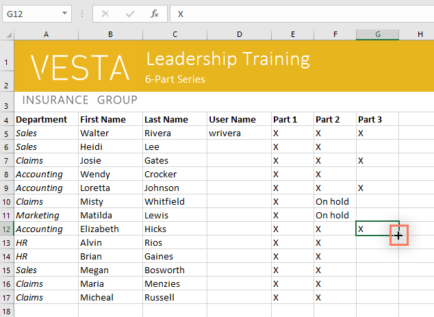
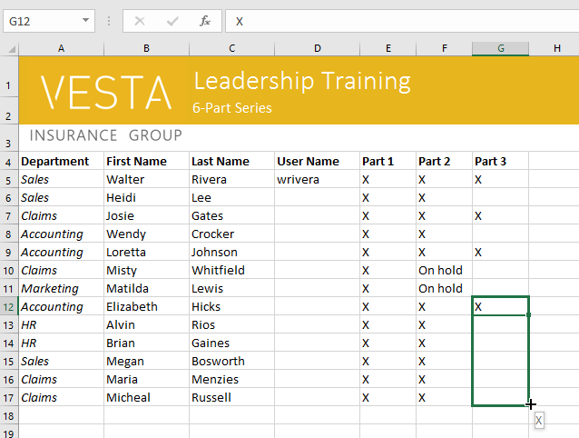
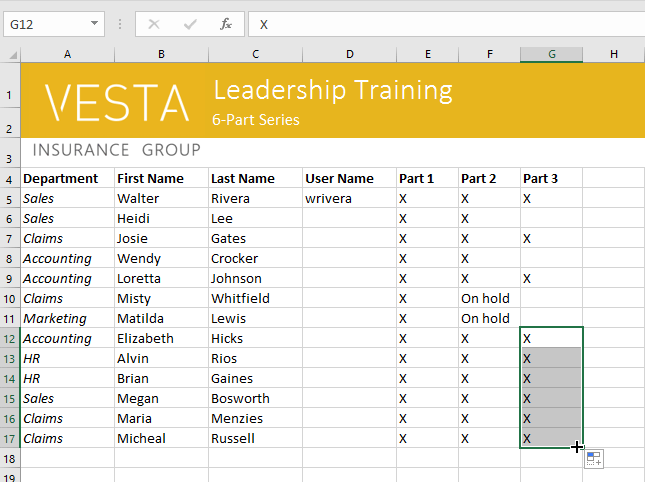
To use the fill handle:
There may be times when you need to copy the content of one cell to several other cells in your worksheet. You could copy and paste the content into each cell, but this method would be time consuming. Instead, you can use the fill handle to quickly copy and paste content to adjacent cells in the same row or column.
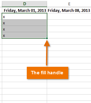
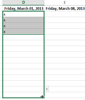
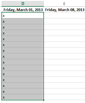
- Select the cell(s) containing the content you want to use. The fill handle will appear as a small square in the bottom-right corner of the selected cell(s).
 Locating the fill handle
 - Click, hold, and drag the fill handle until all of the cells you want to fill are selected.
 Dragging the fill handle
 - Release the mouse to fill the selected cells.
 The filled cells
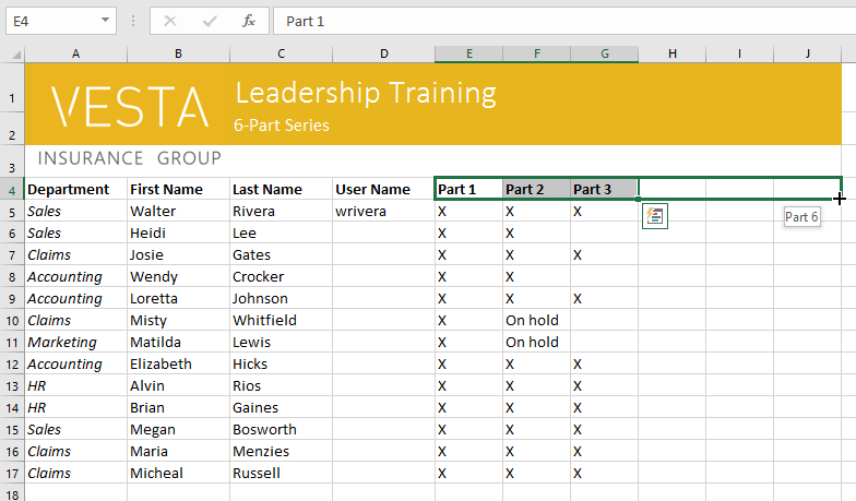
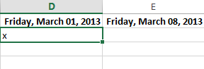
To continue a series with the fill handle:
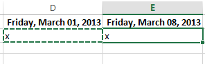
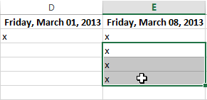
The fill handle can also be used to continue a series. Whenever the content of a row or column follows a sequential order, like numbers (1, 2, 3) or days (Monday, Tuesday, Wednesday), the fill handle can guess what should come next in the series. In many cases, you may need to select multiple cells before using the fill handle to help Excel determine the series order. In our example below, the fill handle is used to extend a series of dates in a column.
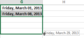 Using the fill handle to extend a series
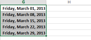 The extended series
You can also double-click the fill handle instead of clicking and dragging. This can be useful with larger spreadsheets, where clicking and dragging may be awkward.
Watch the video below to see an example of double-clicking the fill handle.
To use Flash Fill:
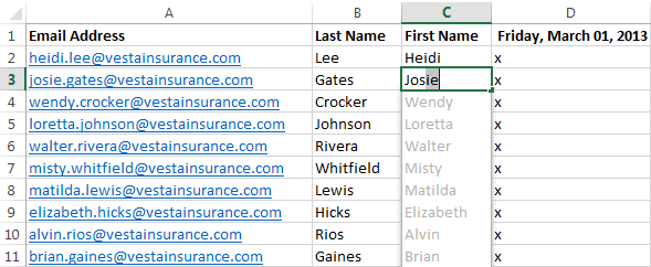
A new feature in Excel 2013, Flash Fill can enter data automatically into your worksheet, saving you time and effort. Just like the fill handle, Flash Fill can guess what type of information you’re entering into your worksheet. In the example below, we’ll use Flash Fill to create a list of first names using a list of existing email addresses.
- Enter the desired information into your worksheet. A Flash Fill preview will appear below the selected cell whenever Flash Fill is available.
 Previewing Flash Fill data
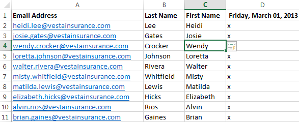
 - Press Enter. The Flash Fill data will be added to the worksheet.
 The entered Flash Fill data
To modify or undo Flash Fill, click the Flash Fill button next to recently added Flash Fill data.
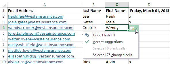 Clicking the Flash Fill button
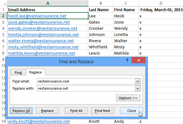
Find and Replace
When working with a lot of data in Excel, it can be difficult and time consuming to locate specific information. You can easily search your workbook using the Find feature, which also allows you to modify content using the Replace feature.
To find content:
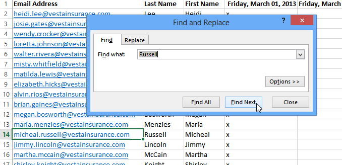
In our example, we’ll use the Find command to locate a specific name in a long list of employees.
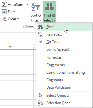
- From the Home tab, click the Find and Select command, then select Find… from the drop-down menu.
 Clicking the Find command
 - The Find and Replace dialog box will appear. Enter the content you want to find. In our example, we’ll type the employee’s name.
- Click Find Next. If the content is found, the cell containing that content will be selected.
 Clicking Find Next
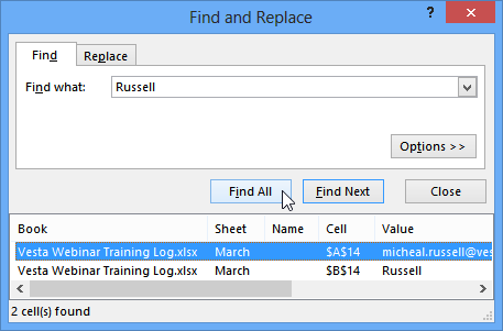
 - Click Find Next to find further instances or Find All to see every instance of the search term.
 Clicking Find All
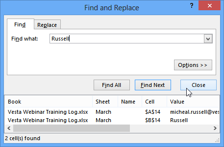
 - When you are finished, click Close to exit the Find and Replace dialog box.
Closing the Find and Replace dialog box
You can also access the Find command by pressing Ctrl+F on your keyboard.
Click Options to see advanced search criteria in the Find and Replace dialog box.
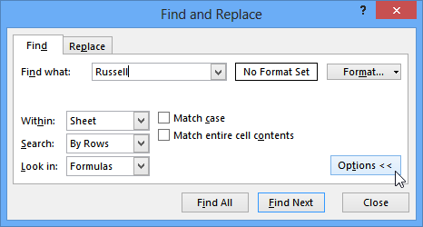 Clicking Options
To replace cell content:
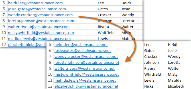
At times, you may discover that you’ve repeatedly made a mistake throughout your workbook (such as misspelling someone’s name), or that you need to exchange a particular word or phrase for another. You can use Excel’s Find and Replace feature to make quick revisions. In our example, we’ll use Find and Replace to correct a list of email addresses.
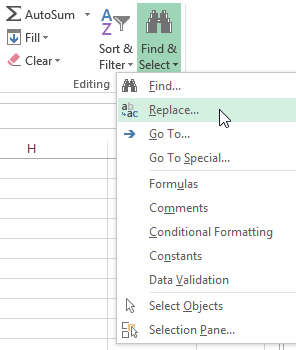
- From the Home tab, click the Find and Select command, then select Replace… from the drop-down menu.
 Clicking the Replace command
 - The Find and Replace dialog box will appear. Type the text you want to find in the Find what: field.
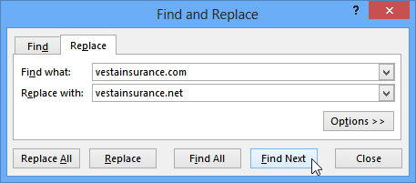
- Type the text you want to replace it with in the Replace with: field, then click Find Next.
 Clicking Find Next
 - If the content is found, the cell containing that content will be selected.
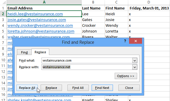
- Review the text to make sure you want to replace it.
- If you want to replace it, select one of the replace options:
- Replace will replace individual instances.
- Replace All will replace every instance of the text throughout the workbook. In our example, we’ll choose this option to save time.
 Replacing the highlighted text
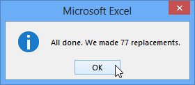
 - A dialog box will appear, confirming the number of replacements made. Click OK to continue.
 Clicking OK
 - The selected cell content will be replaced.
 The replaced content
 - When you are finished, click Close to exit the Find and Replace dialog box.
 Closing the Find and Replace dialog box
Challenge!
- Open an existing Excel 2013 workbook. If you want, you can use our practice workbook.
- Select cell D3. Notice how the cell address appears in the Name box and its content appears in both the cell and the Formula bar.
- Select a cell, and try inserting text and numbers.
- Delete a cell, and note how the cells below shift up to fill in its place.
- Cut cells and paste them into a different location. If you are using the example, cut cells D4:D6 and paste them to E4:E6.
- Try dragging and dropping some cells to other parts of the worksheet.
- Use the fill handle to fill in data to adjoining cells both vertically and horizontally. If you are using the example, use the fill handle to continue the series of dates across row 3.
- Use the Find feature to locate content in your workbook. If you are using the example, type the name Lewis into the Find what: field.
/en/excel2013/modifying-columns-rows-and-cells/content/