
Excel for Microsoft 365 Excel for Microsoft 365 for Mac Excel for the web Excel 2021 Excel 2021 for Mac Excel 2019 Excel 2019 for Mac Excel 2016 Excel 2016 for Mac Excel 2013 Excel 2010 Excel 2007 Excel for Mac 2011 Excel Starter 2010 More…Less
This article describes the formula syntax and usage of the CEILING function in Microsoft Excel.
Description
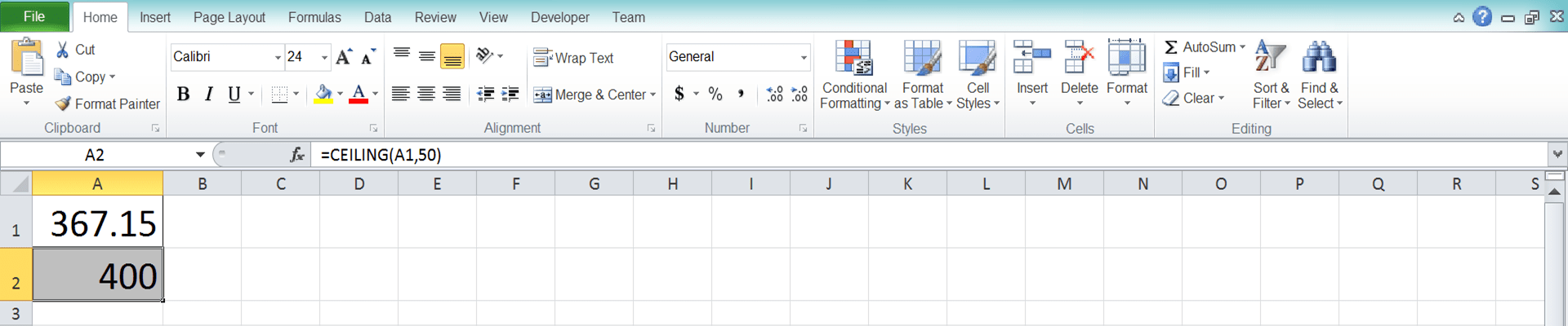
Returns number rounded up, away from zero, to the nearest multiple of significance. For example, if you want to avoid using pennies in your prices and your product is priced at $4.42, use the formula =CEILING(4.42,0.05) to round prices up to the nearest nickel.
Syntax
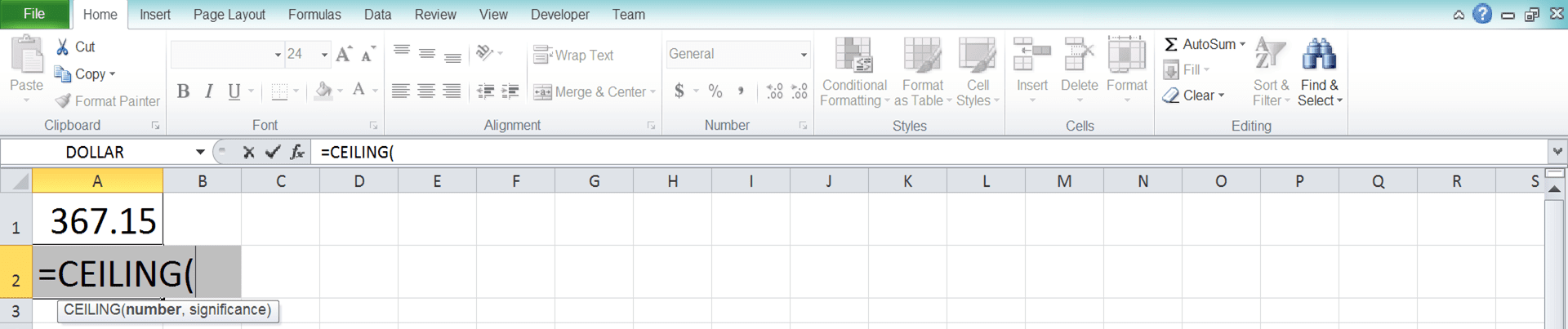
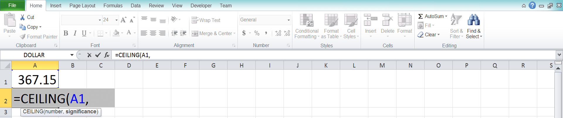
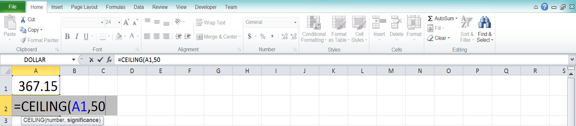
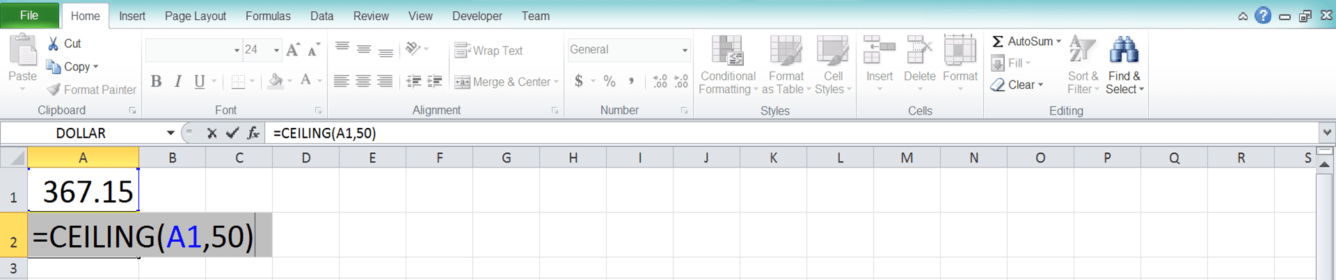
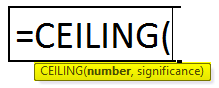
CEILING(number, significance)
The CEILING function syntax has the following arguments:
-
Number Required. The value you want to round.
-
Significance Required. The multiple to which you want to round.
Remarks
-
If either argument is nonnumeric, CEILING returns the #VALUE! error value.
-
Regardless of the sign of number, a value is rounded up when adjusted away from zero. If number is an exact multiple of significance, no rounding occurs.
-
If number is negative, and significance is negative, the value is rounded down, away from zero.
-
If number is negative, and significance is positive, the value is rounded up towards zero.
Example
Copy the example data in the following table, and paste it in cell A1 of a new Excel worksheet. For formulas to show results, select them, press F2, and then press Enter. If you need to, you can adjust the column widths to see all the data.
|
Formula |
Description |
Result |
|---|---|---|
|
=CEILING(2.5, 1) |
Rounds 2.5 up to nearest multiple of 1 |
3 |
|
=CEILING(-2.5, -2) |
Rounds -2.5 up to nearest multiple of -2 |
-4 |
|
=CEILING(-2.5, 2) |
Rounds -2.5 up to nearest multiple of 2 |
-2 |
|
=CEILING(1.5, 0.1) |
Rounds 1.5 up to the nearest multiple of 0.1 |
1.5 |
|
=CEILING(0.234, 0.01) |
Rounds 0.234 up to the nearest multiple of 0.01 |
0.24 |
Need more help?
Excel for Microsoft 365 Excel for Microsoft 365 for Mac Excel for the web Excel 2021 Excel 2021 for Mac Excel 2019 Excel 2019 for Mac Excel 2016 Excel 2016 for Mac Excel 2013 Excel for Mac 2011 More…Less
This article describes the formula syntax and usage of the CEILING.MATH function in Microsoft Excel.
Description
Rounds a number up to the nearest integer or to the nearest multiple of significance.
Syntax
CEILING.MATH(number, [significance], [mode])
The CEILING.MATH function syntax has the following arguments.
-
Number Required. Number must be less than 9.99E+307 and greater than -2.229E-308.
-
Significance Optional. The multiple to which Number is to be rounded.
-
Mode Optional. For negative numbers, controls whether Number is rounded toward or away from zero.
Remarks
-
By default, significance is +1 for positive numbers and -1 for negative numbers.
-
By default, positive numbers with decimal portions are rounded up to the nearest integer. For example, 6.3 is rounded up to 7.
-
By default, negative numbers with decimal portions are rounded up (toward 0) to the nearest integer. For example, -6.7 is rounded up to -6.
-
By specifying the Significance and Mode arguments, you can change the direction of the rounding for negative numbers. For example, rounding -6.3 to a significance of 1 with a mode of 1 rounds away from 0, to -7. There are many combinations of Significance and Mode values that affect rounding of negative numbers in different ways.
-
The Mode argument does not affect positive numbers.
-
The significance argument rounds the number up to the nearest integer that is a multiple of the significance specified. The exception is where the number to be rounded is an integer. For example, for a significance of 3 the number is rounded up to the next integer that is a multiple of 3.
-
If Number divided by a Significance of 2 or greater results in a remainder, the result is rounded up.
Example
Copy the example data in the following table, and paste it in cell A1 of a new Excel worksheet. For formulas to show results, select them, press F2, and then press Enter. If you need to, you can adjust the column widths to see all the data.
|
Formula |
Description |
Result |
|
=CEILING.MATH(24.3,5) |
Rounds 24.3 up to the nearest integer that is a multiple of 5 (25). |
25 |
|
=CEILING.MATH(6.7) |
Rounds 6.7 up to the nearest integer (7). |
7 |
|
=CEILING.MATH(-8.1,2) |
Rounds -8.1 up (toward 0) to the nearest integer that is a multiple of 2 (-8). |
-8 |
|
=CEILING.MATH(-5.5,2,-1) |
Rounds -5.5 down (away from 0) to the nearest integer that is a multiple of 2 with a mode of -1, which reverses rounding direction (-6). |
-6 |
Top of Page
Need more help?
Want more options?
Explore subscription benefits, browse training courses, learn how to secure your device, and more.
Communities help you ask and answer questions, give feedback, and hear from experts with rich knowledge.
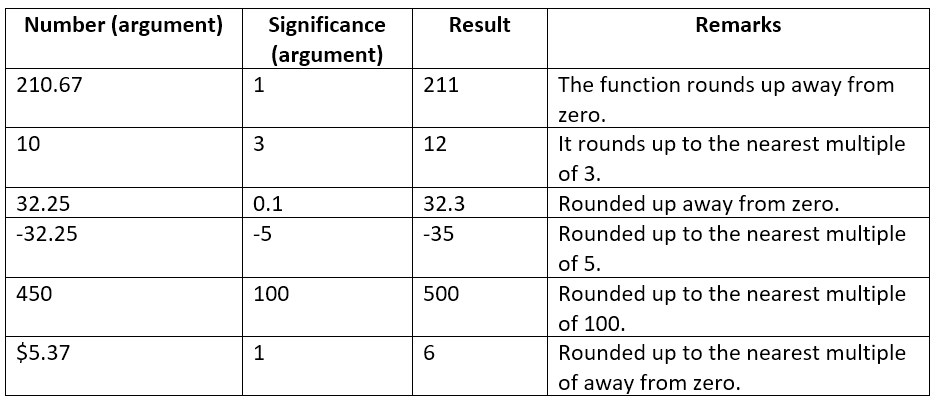
Returns a number rounded up to a supplied number that is away from zero to the nearest multiple of a given number
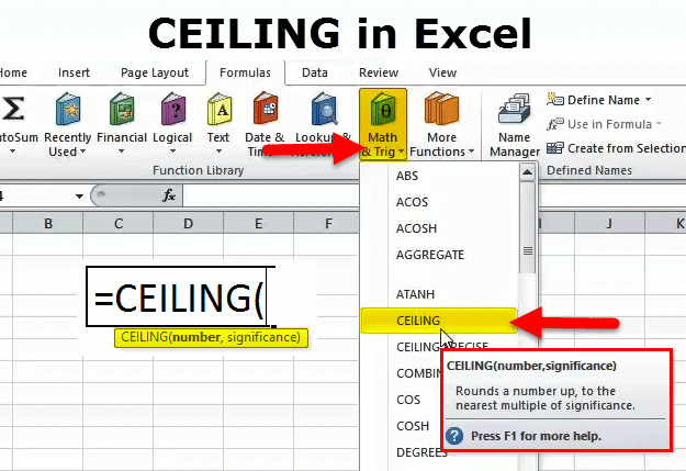
What is the Excel CEILING Function?
The Excel CEILING function[1] is categorized under Math and Trigonometry functions. The function will return a number that is rounded up to a supplied number that is away from zero to the nearest multiple of a given number. MS Excel 2016 handles both positive and negative arguments.
The function is very useful in financial analysis as it helps in setting the price after currency conversion, discounts, etc. When preparing financial models, CEILING helps us round up the numbers as per the requirement. For example, if we provide =CEILING(10,5), the function will round off to the nearest 5 dollars.
Formula
=CEILING(number, significance)
The function uses the following arguments:
- Number (required argument) – This is the value that we wish to round off.
- Significance (required argument) – This is the multiple that we wish to round up to. It would use the same arithmetic sign (positive or negative) as per the provided number argument.
How to use the CEILING Function in Excel
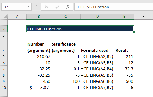
To understand the uses of the CEILING function, let’s consider a few examples:
Example 1 – Excel Ceiling
Let’s see the results from using the function when we provide the following data:
The formula used and results in Excel are shown in the screenshot below:
Example 2 – Using CEILING with other functions
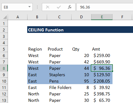
We can use CEILING to highlight rows in a group of data. We will use a combination of ROW, CEILING, and ISEVEN functions. Suppose we are given the data below:
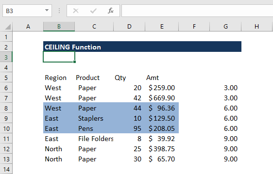
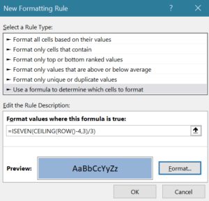
If we wish to highlight rows in groups of 3, we can use the formula =ISEVEN(CEILING(ROW()-4,3)/3) in conditional formatting.
We will get the result below:
In applying the function, remember to select the data before clicking on conditional formatting.
First, we “normalized” the row numbers to begin with 1, using the ROW function and an offset. Here 3 is n (the number of rows to group) and 4 is an offset to normalize the first row to 1 as the first row of data is in row 6. The CEILING function rounds incoming values up to a given multiple of n. Essentially, the CEILING function counts by a given multiple of n.
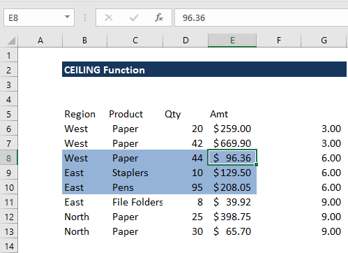
The count shown above in column G is then divided by n, that is in this case =3. Lastly, the ISEVEN function is used to force a TRUE result for all even row groups, which triggers the conditional formatting.
Notes about the Excel CEILING Function
- #NUM! error – Occurs when:
- If we are using MS Excel 2007 or earlier versions, provide the significance argument with a different arithmetic sign from the given number argument.
- If we are using MS Excel 2010 or 2013, if the given number is positive and the supplied significance is negative.
- #DIV/0! error – Occurs when the significance argument provided is 0.
- #VALUE! error – Occurs when any of the arguments is non-numeric.
- CEILING is like MROUND but it always rounds up away from zero.
Click here to download the sample Excel file
Additional Resources
Thanks for reading CFI’s guide to important Excel functions! By taking the time to learn and master these functions, you’ll significantly speed up your financial analysis. To learn more, check out these additional CFI resources:
- Excel Functions for Finance
- Advanced Excel Formulas Course
- Advanced Excel Formulas You Must Know
- Excel Shortcuts for PC and Mac
- See all Excel resources
Article Sources
- CEILING Function
Содержание
- CEILING.MATH function
- Description
- Syntax
- Remarks
- Example
- Excel CEILING Function
- CEILING Function in Excel
- Syntax
- How to Use the CEILING Function in Excel?
- Example #1
- Example #2
- Example #3
- Example #4
- Things to Remember
- Recommended Articles
- CEILING Function
- What is the Excel CEILING Function?
- Formula
- How to use the CEILING Function in Excel
- Example 1 – Excel Ceiling
- Example 2 – Using CEILING with other functions
- Notes about the Excel CEILING Function
- Additional Resources
- How to Use the CEILING Excel Formula: Functions, Examples and Writing Steps
- What is the CEILING Formula in Excel?
- CEILING Function in Excel
- CEILING Result
- Excel Version from Which We Can Use CEILING
- The Way to Write It and Its Inputs
- Example of Its Usage and Result
- Writing Steps
- CEILING to Round Up Date
- CEILING to Round Up Time
- CEILING Alternative: CEILING.MATH
- Exercise
- Questions
- Additional Note
CEILING.MATH function
This article describes the formula syntax and usage of the CEILING.MATH function in Microsoft Excel.
Description
Rounds a number up to the nearest integer or to the nearest multiple of significance.
Syntax
CEILING.MATH(number, [significance], [mode])
The CEILING.MATH function syntax has the following arguments.
Number Required. Number must be less than 9.99E+307 and greater than -2.229E-308.
Significance Optional. The multiple to which Number is to be rounded.
Mode Optional. For negative numbers, controls whether Number is rounded toward or away from zero.
By default, significance is +1 for positive numbers and -1 for negative numbers.
By default, positive numbers with decimal portions are rounded up to the nearest integer. For example, 6.3 is rounded up to 7.
By default, negative numbers with decimal portions are rounded up (toward 0) to the nearest integer. For example, -6.7 is rounded up to -6.
By specifying the Significance and Mode arguments, you can change the direction of the rounding for negative numbers. For example, rounding -6.3 to a significance of 1 with a mode of 1 rounds away from 0, to -7. There are many combinations of Significance and Mode values that affect rounding of negative numbers in different ways.
The Mode argument does not affect positive numbers.
The significance argument rounds the number up to the nearest integer that is a multiple of the significance specified. The exception is where the number to be rounded is an integer. For example, for a significance of 3 the number is rounded up to the next integer that is a multiple of 3.
If Number divided by a Significance of 2 or greater results in a remainder, the result is rounded up.
Example
Copy the example data in the following table, and paste it in cell A1 of a new Excel worksheet. For formulas to show results, select them, press F2, and then press Enter. If you need to, you can adjust the column widths to see all the data.
Rounds 24.3 up to the nearest integer that is a multiple of 5 (25).
Rounds 6.7 up to the nearest integer (7).
Rounds -8.1 up (toward 0) to the nearest integer that is a multiple of 2 (-8).
Rounds -5.5 down (away from 0) to the nearest integer that is a multiple of 2 with a mode of -1, which reverses rounding direction (-6).
Источник
Excel CEILING Function


CEILING Function in Excel
The Excel CEILING function is very similar to the floor function in Excel. Still, the result is just the opposite of the floor function. The floor function gives us the result of the less significance and CEILING formula provides us with the result of higher significance.
So, for example, if we have the number 10 and significance as 3 then 12 will be the result.
Table of contents
Syntax
Compulsory Parameter:
- number: It is the value that you want to round off.
- significance: It is the multiple that we want to round up.
How to Use the CEILING Function in Excel?
Example #1
Let us take a set of positive integers as number arguments and positive numbers as significance, then apply the CEILING Excel function below. It will show the output in the result.

Example #2
In this example, we take a set of negative integers as number arguments and positive numbers as significance, then apply the CEILING Excel formula as shown in the table below. The output will be shown in the result as follows:

Example #3
In this example, we take a set of negative integers as number arguments and negative numbers as significance, then apply the CEILING Excel formula to it.
Example #4
We can use the excel CEILING formula to highlight the rows in the group of given data, as shown in the below table. We will use the CEILING in Excel with ROW and ISEVEN functions.
Suppose we are given the data below:
Things to Remember
- #NUM! error:
- It may occur in MS Excel 2007 or earlier versions. For example, if we provide the significance argument with a different arithmetic sign from the given number argument, get #NUM! Error.
- It occurs if you are using MS Excel 2010/2013, then CEILING functions through #NUM! Error if the given number is positive and the supplied significance is negative.
- #DIV/0! Error occurs when the significance parameter is zero.
- #VALUE! Error occurs when any of the parameters is non-numeric.
- Excel CEILING function is the same as MROUND, but it always rounds up away from zero.
Recommended Articles
This article has been a guide to the CEILING function in Excel. Here we discuss the CEILING formula in Excel and how to use the CEILING function and Excel example, and downloadable Excel templates. You may also look at these useful functions in Excel: –
Источник
CEILING Function
Returns a number rounded up to a supplied number that is away from zero to the nearest multiple of a given number
What is the Excel CEILING Function?
The Excel CEILING function[1] is categorized under Math and Trigonometry functions. The function will return a number that is rounded up to a supplied number that is away from zero to the nearest multiple of a given number. MS Excel 2016 handles both positive and negative arguments.
The function is very useful in financial analysis as it helps in setting the price after currency conversion, discounts, etc. When preparing financial models, CEILING helps us round up the numbers as per the requirement. For example, if we provide =CEILING(10,5), the function will round off to the nearest 5 dollars.
Formula
=CEILING(number, significance)
The function uses the following arguments:
- Number (required argument) – This is the value that we wish to round off.
- Significance (required argument) – This is the multiple that we wish to round up to. It would use the same arithmetic sign (positive or negative) as per the provided number argument.
How to use the CEILING Function in Excel
To understand the uses of the CEILING function, let’s consider a few examples:
Example 1 – Excel Ceiling
Let’s see the results from using the function when we provide the following data:
The formula used and results in Excel are shown in the screenshot below:
Example 2 – Using CEILING with other functions
We can use CEILING to highlight rows in a group of data. We will use a combination of ROW, CEILING, and ISEVEN functions. Suppose we are given the data below:
If we wish to highlight rows in groups of 3, we can use the formula =ISEVEN(CEILING(ROW()-4,3)/3) in conditional formatting.
We will get the result below:
In applying the function, remember to select the data before clicking on conditional formatting.
First, we “normalized” the row numbers to begin with 1, using the ROW function and an offset. Here 3 is n (the number of rows to group) and 4 is an offset to normalize the first row to 1 as the first row of data is in row 6. The CEILING function rounds incoming values up to a given multiple of n. Essentially, the CEILING function counts by a given multiple of n.
The count shown above in column G is then divided by n, that is in this case =3. Lastly, the ISEVEN function is used to force a TRUE result for all even row groups, which triggers the conditional formatting.
Notes about the Excel CEILING Function
- #NUM! error – Occurs when:
- If we are using MS Excel 2007 or earlier versions, provide the significance argument with a different arithmetic sign from the given number argument.
- If we are using MS Excel 2010 or 2013, if the given number is positive and the supplied significance is negative.
- #DIV/0! error – Occurs when the significance argument provided is 0.
- #VALUE! error – Occurs when any of the arguments is non-numeric.
- CEILING is like MROUND but it always rounds up away from zero.
Additional Resources
Thanks for reading CFI’s guide to important Excel functions! By taking the time to learn and master these functions, you’ll significantly speed up your financial analysis. To learn more, check out these additional CFI resources:
Источник
How to Use the CEILING Excel Formula: Functions, Examples and Writing Steps


In this tutorial, you will learn how to use the CEILING excel formula completely.
When working with numbers in excel, we sometimes need to round up a number to a certain multiple. If we use CEILING to do the rounding process, then we can get the result easily!
Want to master the method to use this CEILING formula in excel? Read this tutorial until its last part!
Disclaimer: This post may contain affiliate links from which we earn commission from qualifying purchases/actions at no additional cost for you. Learn more
Want to work faster and easier in Excel? Install and use Excel add-ins! Read this article to know the best Excel add-ins to use according to us!
What is the CEILING Formula in Excel?
CEILING Function in Excel
CEILING Result
Excel Version from Which We Can Use CEILING
The Way to Write It and Its Inputs
Here is the general writing form of a CEILING formula in excel.
And here is the explanation of the inputs we need to give in its formula writing.
- number_to_round = the number we want to round up to a certain multiple
- multiple = the multiple which we round up our number to
Example of Its Usage and Result
Here is the usage and result example of the CEILING formula in excel.
As you can see there, CEILING will always round up the number we input into it to the multiple we want. When we input negative numbers, CEILING will round our number away from zero.
Writing Steps
After discussing the writing form, inputs, and implementation example of CEILING, now let’s discuss its writing steps. As the inputs of this formula are quite simple, you should be able to understand the writing steps easily!
- Type an equal sign ( = ) in the cell where you want to put your CEILING result
Type CEILING (can be with large and small letters) and an open bracket sign after =
Input the number you want to round up to a certain multiple. Then, type a comma sign ( , )
Input the multiple you want to round up your number to
Type a close bracket sign
CEILING to Round Up Date
As the date is also a number data, we can use CEILING to round it up to a certain days multiple. Just input the date we want to round up and the days multiple we want to round our date to.
Here is the CEILING general writing form in excel to round up a date.
And here is its implementation example.
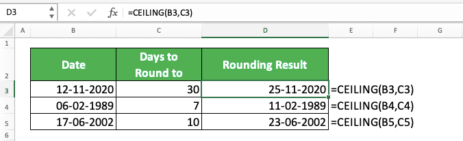
If you get a number from CEILING when you round up your date, just change its data type to date.
CEILING to Round Up Time
As time is a number data too, we can also round up time data using CEILING. Just input the time data you want to round up and the time multiple you want to round it to.
The time multiple you input to CEILING to round up time can be in hours, minutes, or seconds. Input it in the form of time data too so you can get your result correctly.
Here is the CEILING general writing form in excel to round up time.
And here is its implementation example.
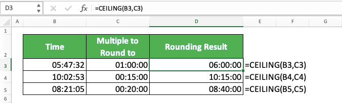
Similar to date, if you get a number from CEILING instead of time, you should change the data type to time.
CEILING Alternative: CEILING.MATH
Since excel 2013, you can use CEILING.MATH as an alternative to CEILING.
If we look at the basic function, CEILING.MATH is the same as CEILING. They both help you to round up your number to a certain multiple.
There are two things, however, that become crucial differences when it comes to CEILING and CEILING.MATH.
- CEILING doesn’t have a default multiple input. That means you have to input a multiple to CEILING for the formula to run.
CEILING.MATH, meanwhile, has a default multiple input of 1. If you don’t give any multiple input to CEILING.MATH, it will round up your number to the multiple of 1
You can control your negative number rounding process with CEILING.MATH while you can’t do that with CEILING. If you use CEILING, you will round your negative number away from zero.
If you use CEILING.MATH, however, you can input whether you want to round it closer to or away from zero
Here is the general writing form of CEILING.MATH in excel.
You have one required input and two optional inputs in CEILING.MATH. For the required input, you must input the number you want to round as the first input of your CEILING.MATH.
For the negative number rounding mode, the default is you round your negative number closer to zero. If you input any non-zero value for it, you will round your negative number away from zero. If you input zero or don’t input anything, you will round it closer to zero.
For a better understanding of the formula, here is the implementation example of CEILING.MATH in excel.
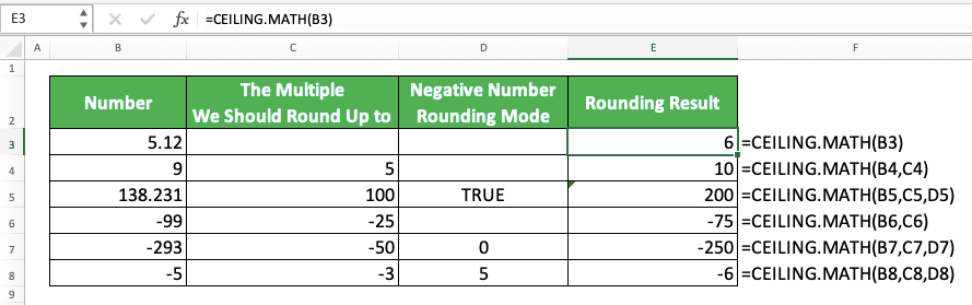
As you can see in the example, CEILING and CEILING.MATH round up positive numbers the same way. When we don’t input a multiple to CEILING.MATH, it will round our number up to the multiple of 1.
When we round a negative number, however, the default nature of CEILING.MATH is to round it closer to zero (the opposite of CEILING). We can input a non-zero value as its negative number rounding mode to round our negative number away from zero (TRUE is the same as 1 in excel, hence the rounding result for the third number in the example).
When you need the differences that CEILING.MATH gives, use it in your formula writing!
Exercise
After you have learned how to use the CEILING in excel, you can sharpen your understanding by doing the exercise below!
Download the exercise file from the following link and answer the questions. Download the answer key file to compare your answers with if you have done the exercise.
Link to the exercise file:
Download here
Questions
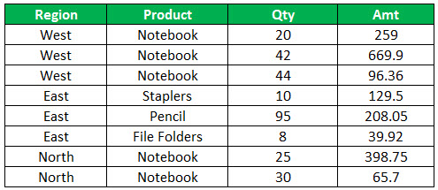
- What is the production quantity for the benchmark of the company’s factory if the standard batch is 10?
- What is the production quantity for the benchmark of the company’s factory if the standard batch is 50?
- What is the production quantity for the benchmark of the company’s factory if the standard batch is 1000?
Link to the answer key file:
Download here
Additional Note
If you round up a positive number to a negative multiple using CEILING, you will get a #NUM error.
Related tutorials you should learn from:
Источник
CEILING Function (Table of Contents)
- CEILING in Excel
- CEILING Formula in Excel
- How to use the CEILING Function in Excel?
Introduction to CEILING in Excel
The ceiling function is another mathematical function in excel which is quite useful which is used for rounding off any decimal number closer to the value selected in the function but away from 0. RND function rounds off any decimal value to a whole number, whereas in the Ceiling function, we can choose the number to which extent we want to see the decimal number. We can either get the whole number or value in 0.5 formats.
In simple terms, you are providing both number and significance number, and you are asking Excel to round up the given to the nearest multiple of given significance number.
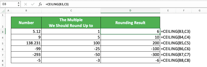
For example: If the formula reads =CEILING (22, 8), it will return the value of 24. Now, let us break down the formula.
If you multiply 8 with 3, the resulting number is 24. The supplied number is 22 what is the nearest multiple numbers of 8.
8 * 1 = 8 (Not nearest to 22)
8 * 2 = 16 (Not nearest to 22)
8 * 3 =24 (Nearest to 22)
8 * 4 = 32 (Too far from 22)
So CEILING function returns the nearest multiple of significance number to the nearest supplied number.
CEILING Formula in Excel:
The Formula for the CEILING function is as follows:
The Formula of CEILING function includes 2 arguments.
- Number: It is a mandatory argument. The number you want to round up.
- Significance: This is also a required argument. This is the number you are multiplying to round up the first given number.
How to Use CEILING Function in Excel?
CEILING in Excel is very simple and easy to use. Let us understand the working of the CEILING function by some examples.
You can download this CEILING Function Excel Template here – CEILING Function Excel Template
Example 1
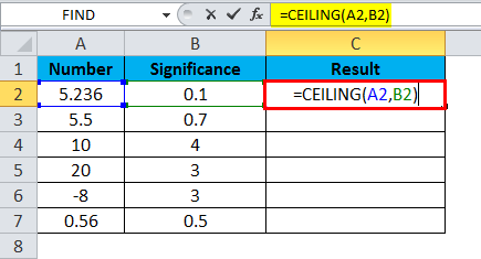
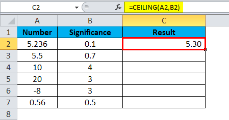
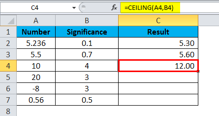
In the below image, I have applied the CEILING function to the numbers from A2:A7. I will discuss this one by one.
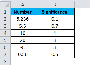
- In the first formula, the given number is 5.236, and the significance we are giving is 0.1. Formula used is =CEILING(A2,B2)
Formula returned the value of 5.3, which means the formula rounded up the 5.236 to the next nearest multiple of 0.1, i.e. 5.30.
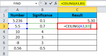
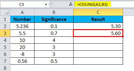
- In the second formula, we are rounding up the 5.5 to the next decimal number, i.e. 5.6. The formula used is =CEILING(A3,B3)
The significance we have given is 0.7, i.e. 0.7*8=5.60.
- Now look at the third formula number is 10, and the significant number is 4. One thing you need to observe here is 4*2=8 (this is also nearest to 10) and 4*3=12 (this is also nearest to 10). The formula used is =CEILING(A4,B4)
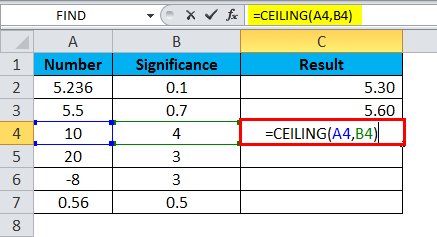
CEILING always returns the next nearest number. O, the result of the formula is 12.
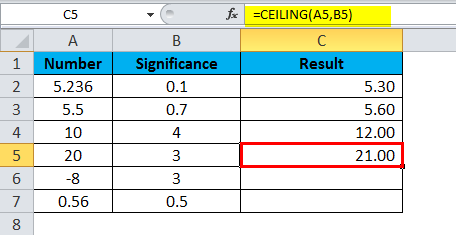
- The fourth formula number is 20, and the significant number is 3, i.e. 3*7 = 21, which is nearest to 20. Formula used is =CEILING(A5,B5)
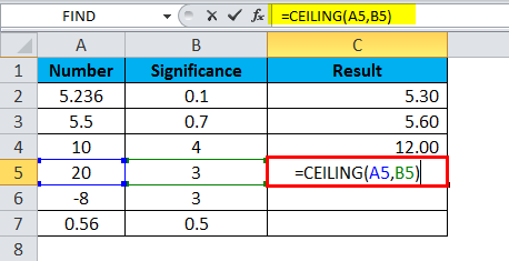
The result of the formula is 21.
- CEILING also works for negative numbers too. In the fifth formula, the number is negative (-8), and the significance is positive (3). 3*3 = 9, which is nearest to 8. The Formula used is =CEILING(A6,B6)
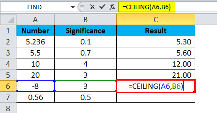
Since it is a negative number, the formula returns the lower value, i.e. 3*2=6, and the supplied number is negative; the result also will be negative only (-6).
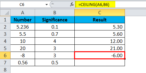
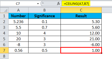
- Final formula is 0.5*2 = 1 that is round up of 0.56. 0.5*1 = 0.5 only this is lower than the original value of 0.56. Formula used is =CEILING(A7,B7)
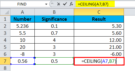
The next highest value is 1.
Example 2
In the first example, we have seen positive numbers with positive significance. In this example, I will explain the scenarios of negative numbers with positive significance.
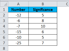
Negative numbers always round down the values, unlike positive numbers, which always round up the values.
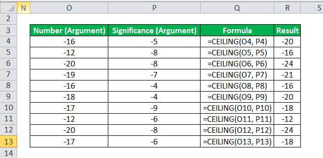
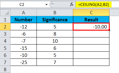
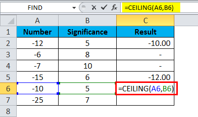
- In the first formula, the number is -12, and the significance is 5. Formula used is =CEILING(A2,B2)
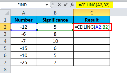
Significance multiple is 5*2 = -10 which is nearest to -12 unlike 5*3 =-15.
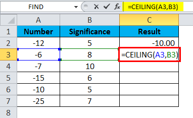
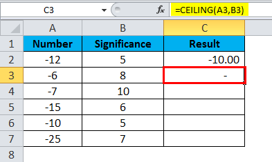
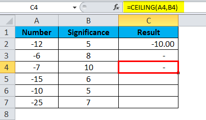
- The second formula returns 0; the reason behind this is the given number is -6, but we are multiplying values is 8, which always returns the value of more than 6. The formula used is =CEILING(A3,B3).
Therefore, the formula returns nothing.
- Third, one is also the same as the second one. The significant number is more than the given number. Formula used is = CEILING(A4,B4).
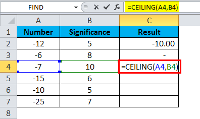
The result will be zero.
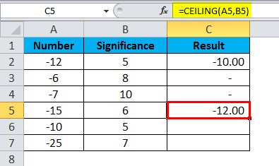
- In the fourth formula, a number is -15, and significance is 6. A formula used is =CEILING(A5,B5).
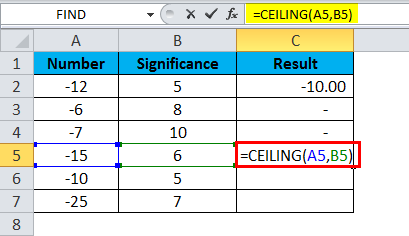
Significance multiple is 6*2 = -12 which is nearest to -15 unlike 6*3 =-18.
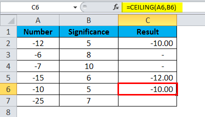
- In the fifth formula, a number is -10, and significance is 5. The formula used is =CEILING(6,B6).
The significance multiple is 5*2 = -10, which is equal to the given number.
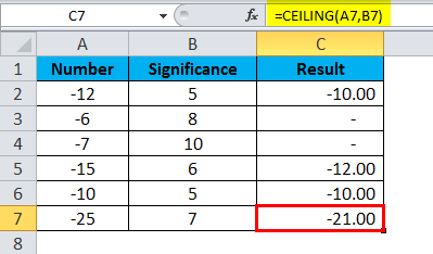
- In the sixth formula, the number is -25, and the significance is 7. The formula used is =CEILING(A7,B7).
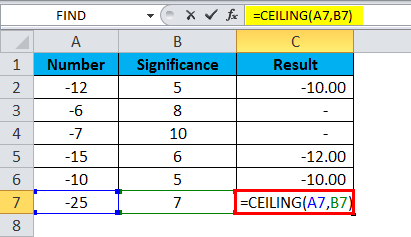
Significance multiple is 3*3 = -21 which is nearest to -25 unlike 7*4 =-28.
Things to Remember
- In this function, the number always gets larger, i.e. round up always based on the multiple of significance number.
- The number should not be less than the significance numbers; otherwise, the result would always be zero.
- This formula does not accept values other than numeric values. If anyone of the supplied argument is non-numeric, then the result will be #VALUE!
- The number is positive, and the significant number is negative, then we will get the error as #NUM! Therefore, if the significant number is negative, then the number also should be negative.
Recommended Articles
This has been a guide to the CEILING Function. Here we discuss the CEILING Formula and how to use the CEILING function along with a practical example and downloadable excel templates. You may also look at these useful functions in excel –
- MID Function in Excel
- SUM Function in Excel
- POWER Function in Excel
- SUBSTITUTE Function in Excel