What is array function in excel - Word и Excel - помощь в работе с программами

An array formula is a formula that can perform multiple calculations on one or more items in an array. You can think of an array as a row or column of values, or a combination of rows and columns of values. Array formulas can return either multiple results, or a single result.

Beginning with the September 2018 update for Microsoft 365, any formula that can return multiple results will automatically spill them either down, or across into neighboring cells. This change in behavior is also accompanied by several new dynamic array functions. Dynamic array formulas, whether they’re using existing functions or the dynamic array functions, only need to be input into a single cell, then confirmed by pressing Enter. Earlier, legacy array formulas require first selecting the entire output range, then confirming the formula with Ctrl+Shift+Enter. They’re commonly referred to as CSE formulas.

You can use array formulas to perform complex tasks, such as:

Quickly create sample datasets.
Count the number of characters contained in a range of cells.
Sum only numbers that meet certain conditions, such as the lowest values in a range, or numbers that fall between an upper and lower boundary.
Sum every Nth value in a range of values.

The following examples show you how to create multi-cell and single-cell array formulas. Where possible, we’ve included examples with some of the dynamic array functions, as well as existing array formulas entered as both dynamic and legacy arrays.

Download our examples

Download an example workbook with all the array formula examples in this article.

This exercise shows you how to use multi-cell and single-cell array formulas to calculate a set of sales figures. The first set of steps uses a multi-cell formula to calculate a set of subtotals. The second set uses a single-cell formula to calculate a grand total.

Multi-cell array formula
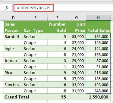
Here we’re calculating Total Sales of coupes and sedans for each salesperson by entering =F10:F19*G10:G19 in cell H10.

When you press Enter, you’ll see the results spill down to cells H10:H19. Notice that the spill range is highlighted with a border when you select any cell within the spill range. You might also notice that the formulas in cells H10:H19 are grayed out. They’re just there for reference, so if you want to adjust the formula, you’ll need to select cell H10, where the master formula lives.
Single-cell array formula

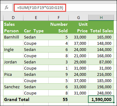
In cell H20 of the example workbook, type or copy and paste =SUM(F10:F19*G10:G19), and then press Enter.

In this case, Excel multiplies the values in the array (the cell range F10 through G19), and then uses the SUM function to add the totals together. The result is a grand total of $1,590,000 in sales.

This example shows how powerful this type of formula can be. For example, suppose you have 1,000 rows of data. You can sum part or all of that data by creating an array formula in a single cell instead of dragging the formula down through the 1,000 rows. Also, notice that the single-cell formula in cell H20 is completely independent of the multi-cell formula (the formula in cells H10 through H19). This is another advantage of using array formulas — flexibility. You could change the other formulas in column H without affecting the formula in H20. It can also be good practice to have independent totals like this, as it helps validate the accuracy of your results.
Dynamic array formulas also offer these advantages:
- Consistency If you click any of the cells from H10 downward, you see the same formula. That consistency can help ensure greater accuracy.
- Safety You can’t overwrite a component of a multi-cell array formula. For example, click cell H11 and press Delete. Excel won’t change the array’s output. To change it, you need to select the top-left cell in the array, or cell H10.
- Smaller file sizes You can often use a single array formula instead of several intermediate formulas. For example, the car sales example uses one array formula to calculate the results in column E. If you had used standard formulas such as =F10*G10, F11*G11, F12*G12, etc., you would have used 11 different formulas to calculate the same results. That’s not a big deal, but what if you had thousands of rows to total? Then it can make a big difference.
- Efficiency Array functions can be an efficient way to build complex formulas. The array formula =SUM(F10:F19*G10:G19) is the same as this: =SUM(F10*G10,F11*G11,F12*G12,F13*G13,F14*G14,F15*G15,F16*G16,F17*G17,F18*G18,F19*G19).
- Spilling Dynamic array formulas will automatically spill into the output range. If your source data is in an Excel table, then your dynamic array formulas will automatically resize as you add or remove data.
- #SPILL! error Dynamic arrays introduced the #SPILL! error, which indicates that the intended spill range is blocked for some reason. When you resolve the blockage, the formula will automatically spill.

Array constants are a component of array formulas. You create array constants by entering a list of items and then manually surrounding the list with braces ({ }), like this:

={1,2,3,4,5} or ={«January»,»February»,»March»}

If you separate the items by using commas, you create a horizontal array (a row). If you separate the items by using semicolons, you create a vertical array (a column). To create a two-dimensional array, you delimit the items in each row with commas, and delimit each row with semicolons.

The following procedures will give you some practice in creating horizontal, vertical, and two-dimensional constants. We’ll show examples using the SEQUENCE function to automatically generate array constants, as well as manually entered array constants.

Create a horizontal constant

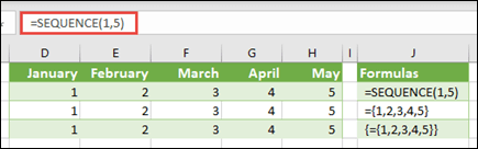
Use the workbook from the previous examples, or create a new workbook. Select any empty cell and enter =SEQUENCE(1,5). The SEQUENCE function builds a 1 row by 5 column array the same as ={1,2,3,4,5}. The following result is displayed:
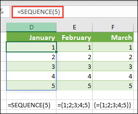
Create a vertical constant

Select any blank cell with room beneath it, and enter =SEQUENCE(5), or ={1;2;3;4;5}. The following result is displayed:
Create a two-dimensional constant

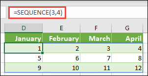
Select any blank cell with room to the right and beneath it, and enter =SEQUENCE(3,4). You see the following result:

You can also enter: or ={1,2,3,4;5,6,7,8;9,10,11,12}, but you’ll want to pay attention to where you put semi-colons versus commas.

As you can see, the SEQUENCE option offers significant advantages over manually entering your array constant values. Primarily, it saves you time, but it can also help reduce errors from manual entry. It’s also easier to read, especially as the semi-colons can be hard to distinguish from the comma separators.

Here’s an example that uses array constants as part of a bigger formula. In the sample workbook, go to the Constant in a formula worksheet, or create a new worksheet.

In cell D9, we entered =SEQUENCE(1,5,3,1), but you could also enter 3, 4, 5, 6, and 7 in cells A9:H9. There’s nothing special about that particular number selection, we just chose something other than 1-5 for differentiation.

In cell E11, enter =SUM(D9:H9*SEQUENCE(1,5)), or =SUM(D9:H9*{1,2,3,4,5}). The formulas return 85.

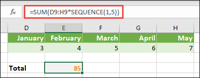
The SEQUENCE function builds the equivalent of the array constant {1,2,3,4,5}. Because Excel performs operations on expressions enclosed in parentheses first, the next two elements that come into play are the cell values in D9:H9, and the multiplication operator (*). At this point, the formula multiplies the values in the stored array by the corresponding values in the constant. It’s the equivalent of:

=SUM(D9*1,E9*2,F9*3,G9*4,H9*5), or =SUM(3*1,4*2,5*3,6*4,7*5)

Finally, the SUM function adds the values, and returns 85.

To avoid using the stored array and keep the operation entirely in memory, you can replace it with another array constant:

=SUM(SEQUENCE(1,5,3,1)*SEQUENCE(1,5)), or =SUM({3,4,5,6,7}*{1,2,3,4,5})

Elements that you can use in array constants

Array constants can contain numbers, text, logical values (such as TRUE and FALSE), and error values such as #N/A. You can use numbers in integer, decimal, and scientific formats. If you include text, you need to surround it with quotation marks («text”).
Array constants can’t contain additional arrays, formulas, or functions. In other words, they can contain only text or numbers that are separated by commas or semicolons. Excel displays a warning message when you enter a formula such as {1,2,A1:D4} or {1,2,SUM(Q2:Z8)}. Also, numeric values can’t contain percent signs, dollar signs, commas, or parentheses.

One of the best ways to use array constants is to name them. Named constants can be much easier to use, and they can hide some of the complexity of your array formulas from others. To name an array constant and use it in a formula, do the following:

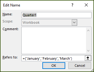
Go to Formulas > Defined Names > Define Name. In the Name box, type Quarter1. In the Refers to box, enter the following constant (remember to type the braces manually):

={«January»,»February»,»March»}

The dialog box should now look like this:

Click OK, then select any row with three blank cells, and enter =Quarter1.

The following result is displayed:

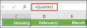
If you want the results to spill vertically instead of horizontally, you can use =TRANSPOSE(Quarter1).

If you want to display a list of 12 months, like you might use when building a financial statement, you can base one off the current year with the SEQUENCE function. The neat thing about this function is that even though only the month is displaying, there is a valid date behind it that you can use in other calculations. You’ll find these examples on the Named array constant and Quick sample dataset worksheets in the example workbook.

=TEXT(DATE(YEAR(TODAY()),SEQUENCE(1,12),1),»mmm»)

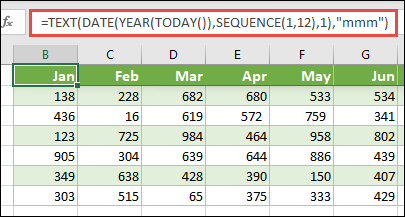
This uses the DATE function to create a date based on the current year, SEQUENCE creates an array constant from 1 to 12 for January through December, then the TEXT function converts the display format to «mmm» (Jan, Feb, Mar, etc.). If you wanted to display the full month name, such as January, you’d use «mmmm».

When you use a named constant as an array formula, remember to enter the equal sign, as in =Quarter1, not just Quarter1. If you don’t, Excel interprets the array as a string of text and your formula won’t work as expected. Finally, keep in mind that you can use combinations of functions, text and numbers. It all depends on how creative you want to get.

The following examples demonstrate a few of the ways in which you can put array constants to use in array formulas. Some of the examples use the TRANSPOSE function to convert rows to columns and vice versa.

Multiple each item in an array

Enter =SEQUENCE(1,12)*2, or ={1,2,3,4;5,6,7,8;9,10,11,12}*2

You can also divide with (/), add with (+), and subtract with (—).
Square the items in an array

Enter =SEQUENCE(1,12)^2, or ={1,2,3,4;5,6,7,8;9,10,11,12}^2
Find the square root of squared items in an array

Enter =SQRT(SEQUENCE(1,12)^2), or =SQRT({1,2,3,4;5,6,7,8;9,10,11,12}^2)
Transpose a one-dimensional row

Enter =TRANSPOSE(SEQUENCE(1,5)), or =TRANSPOSE({1,2,3,4,5})

Even though you entered a horizontal array constant, the TRANSPOSE function converts the array constant into a column.
Transpose a one-dimensional column

Enter =TRANSPOSE(SEQUENCE(5,1)), or =TRANSPOSE({1;2;3;4;5})

Even though you entered a vertical array constant, the TRANSPOSE function converts the constant into a row.
Transpose a two-dimensional constant

Enter =TRANSPOSE(SEQUENCE(3,4)), or =TRANSPOSE({1,2,3,4;5,6,7,8;9,10,11,12})

The TRANSPOSE function converts each row into a series of columns.

This section provides examples of basic array formulas.

Create an array from existing values

The following example explains how to use array formulas to create a new array from an existing array.

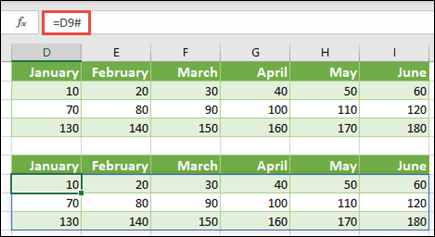
Enter =SEQUENCE(3,6,10,10), or ={10,20,30,40,50,60;70,80,90,100,110,120;130,140,150,160,170,180}

Be sure to type { (opening brace) before you type 10, and } (closing brace) after you type 180, because you’re creating an array of numbers.

Next, enter =D9#, or =D9:I11 in a blank cell. A 3 x 6 array of cells appears with the same values you see in D9:D11. The # sign is called the spilled range operator, and it’s Excel’s way of referencing the entire array range instead of having to type it out.
Create an array constant from existing values

You can take the results of a spilled array formula and convert that into its component parts. Select cell D9, then press F2 to switch to edit mode. Next, press F9 to convert the cell references to values, which Excel then converts into an array constant. When you press Enter, the formula, =D9#, should now be ={10,20,30;40,50,60;70,80,90}.
Count characters in a range of cells

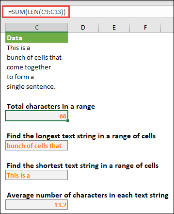
The following example shows you how to count the number of characters in a range of cells. This includes spaces.

=SUM(LEN(C9:C13))

In this case, the LEN function returns the length of each text string in each of the cells in the range. The SUM function then adds those values together and displays the result (66). If you wanted to get average number of characters, you could use:

=AVERAGE(LEN(C9:C13))
Contents of longest cell in range C9:C13

=INDEX(C9:C13,MATCH(MAX(LEN(C9:C13)),LEN(C9:C13),0),1)

This formula works only when a data range contains a single column of cells.

Let’s take a closer look at the formula, starting from the inner elements and working outward. The LEN function returns the length of each of the items in the cell range D2:D6. The MAX function calculates the largest value among those items, which corresponds to the longest text string, which is in cell D3.

Here’s where things get a little complex. The MATCH function calculates the offset (the relative position) of the cell that contains the longest text string. To do that, it requires three arguments: a lookup value, a lookup array, and a match type. The MATCH function searches the lookup array for the specified lookup value. In this case, the lookup value is the longest text string:

MAX(LEN(C9:C13)

and that string resides in this array:

LEN(C9:C13)

The match type argument in this case is 0. The match type can be a 1, 0, or -1 value.
- 1 — returns the largest value that is less than or equal to the lookup val
- 0 — returns the first value exactly equal to the lookup value
- -1 — returns the smallest value that is greater than or equal to the specified lookup value
- If you omit a match type, Excel assumes 1.
Finally, the INDEX function takes these arguments: an array, and a row and column number within that array. The cell range C9:C13 provides the array, the MATCH function provides the cell address, and the final argument (1) specifies that the value comes from the first column in the array.

If you wanted to get the contents of the smallest text string, you would replace MAX in the above example with MIN.
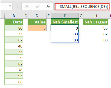
Find the n smallest values in a range

This example shows how to find the three smallest values in a range of cells, where an array of sample data in cells B9:B18has been created with: =INT(RANDARRAY(10,1)*100). Note that RANDARRAY is a volatile function, so you’ll get a new set of random numbers each time Excel calculates.

Enter =SMALL(B9#,SEQUENCE(D9), =SMALL(B9:B18,{1;2;3})

This formula uses an array constant to evaluate the SMALL function three times and return the smallest 3 members in the array that’s contained in cells B9:B18, where 3 is a variable value in cell D9. To find more values, you can increase the value in the SEQUENCE function, or add more arguments to the constant. You can also use additional functions with this formula, such as SUM or AVERAGE. For example:

=SUM(SMALL(B9#,SEQUENCE(D9))

=AVERAGE(SMALL(B9#,SEQUENCE(D9))
Find the n largest values in a range

To find the largest values in a range, you can replace the SMALL function with the LARGE function. In addition, the following example uses the ROW and INDIRECT functions.

Enter =LARGE(B9#,ROW(INDIRECT(«1:3»))), or =LARGE(B9:B18,ROW(INDIRECT(«1:3»)))

At this point, it may help to know a bit about the ROW and INDIRECT functions. You can use the ROW function to create an array of consecutive integers. For example, select an empty and enter:

=ROW(1:10)

The formula creates a column of 10 consecutive integers. To see a potential problem, insert a row above the range that contains the array formula (that is, above row 1). Excel adjusts the row references, and the formula now generates integers from 2 to 11. To fix that problem, you add the INDIRECT function to the formula:

=ROW(INDIRECT(«1:10»))

The INDIRECT function uses text strings as its arguments (which is why the range 1:10 is surrounded by quotation marks). Excel does not adjust text values when you insert rows or otherwise move the array formula. As a result, the ROW function always generates the array of integers that you want. You could just as easily use SEQUENCE:

=SEQUENCE(10)

Let’s examine the formula that you used earlier — =LARGE(B9#,ROW(INDIRECT(«1:3»))) — starting from the inner parentheses and working outward: The INDIRECT function returns a set of text values, in this case the values 1 through 3. The ROW function in turn generates a three-cell column array. The LARGE function uses the values in the cell range B9:B18, and it is evaluated three times, once for each reference returned by the ROW function. If you want to find more values, you add a greater cell range to the INDIRECT function. Finally, as with the SMALL examples, you can use this formula with other functions, such as SUM and AVERAGE.

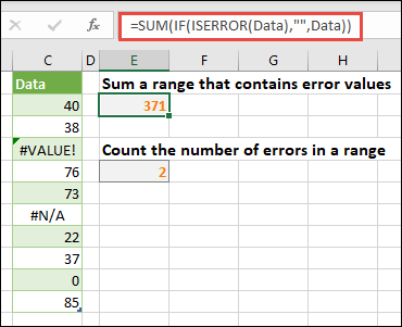
Sum a range that contains error values

The SUM function in Excel does not work when you try to sum a range that contains an error value, such as #VALUE! or #N/A. This example shows you how to sum the values in a range named Data that contains errors:
=SUM(IF(ISERROR(Data),»»,Data))

The formula creates a new array that contains the original values minus any error values. Starting from the inner functions and working outward, the ISERROR function searches the cell range (Data) for errors. The IF function returns a specific value if a condition you specify evaluates to TRUE and another value if it evaluates to FALSE. In this case, it returns empty strings («») for all error values because they evaluate to TRUE, and it returns the remaining values from the range (Data) because they evaluate to FALSE, meaning that they don’t contain error values. The SUM function then calculates the total for the filtered array.
Count the number of error values in a range

This example is like the previous formula, but it returns the number of error values in a range named Data instead of filtering them out:

=SUM(IF(ISERROR(Data),1,0))

This formula creates an array that contains the value 1 for the cells that contain errors and the value 0 for the cells that don’t contain errors. You can simplify the formula and achieve the same result by removing the third argument for the IF function, like this:

=SUM(IF(ISERROR(Data),1))

If you don’t specify the argument, the IF function returns FALSE if a cell does not contain an error value. You can simplify the formula even more:

=SUM(IF(ISERROR(Data)*1))

This version works because TRUE*1=1 and FALSE*1=0.

You might need to sum values based on conditions.

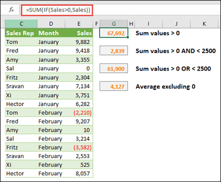
For example, this array formula sums just the positive integers in a range named Sales, which represents cells E9:E24 in the example above:

=SUM(IF(Sales>0,Sales))

The IF function creates an array of positive and false values. The SUM function essentially ignores the false values because 0+0=0. The cell range that you use in this formula can consist of any number of rows and columns.

You can also sum values that meet more than one condition. For example, this array formula calculates values greater than 0 AND less than 2500:

=SUM((Sales>0)*(Sales<2500)*(Sales))

Keep in mind that this formula returns an error if the range contains one or more non-numeric cells.

You can also create array formulas that use a type of OR condition. For example, you can sum values that are greater than 0 OR less than 2500:

=SUM(IF((Sales>0)+(Sales<2500),Sales))

You can’t use the AND and OR functions in array formulas directly because those functions return a single result, either TRUE or FALSE, and array functions require arrays of results. You can work around the problem by using the logic shown in the previous formula. In other words, you perform math operations, such as addition or multiplication on values that meet the OR or AND condition.

This example shows you how to remove zeros from a range when you need to average the values in that range. The formula uses a data range named Sales:

=AVERAGE(IF(Sales<>0,Sales))

The IF function creates an array of values that do not equal 0 and then passes those values to the AVERAGE function.

This array formula compares the values in two ranges of cells named MyData and YourData and returns the number of differences between the two. If the contents of the two ranges are identical, the formula returns 0. To use this formula, the cell ranges need to be the same size and of the same dimension. For example, if MyData is a range of 3 rows by 5 columns, YourData must also be 3 rows by 5 columns:

=SUM(IF(MyData=YourData,0,1))

The formula creates a new array of the same size as the ranges that you are comparing. The IF function fills the array with the value 0 and the value 1 (0 for mismatches and 1 for identical cells). The SUM function then returns the sum of the values in the array.

You can simplify the formula like this:

=SUM(1*(MyData<>YourData))

Like the formula that counts error values in a range, this formula works because TRUE*1=1, and FALSE*1=0.

This array formula returns the row number of the maximum value in a single-column range named Data:

=MIN(IF(Data=MAX(Data),ROW(Data),»»))

The IF function creates a new array that corresponds to the range named Data. If a corresponding cell contains the maximum value in the range, the array contains the row number. Otherwise, the array contains an empty string («»). The MIN function uses the new array as its second argument and returns the smallest value, which corresponds to the row number of the maximum value in Data. If the range named Data contains identical maximum values, the formula returns the row of the first value.

If you want to return the actual cell address of a maximum value, use this formula:

=ADDRESS(MIN(IF(Data=MAX(Data),ROW(Data),»»)),COLUMN(Data))

You’ll find similar examples in the sample workbook on the Differences between datasets worksheet.

Multi-cell array formula

Copy the entire table below and paste it into cell A1 in a blank worksheet.

Sales Person	Car Type	Number Sold	Unit Price
Barnhill	Sedan	5	33000
	Coupe	4	37000
Ingle	Sedan	6	24000
	Coupe	8	21000
Jordan	Sedan	3	29000
	Coupe	1	31000
Pica	Sedan	9	24000
	Coupe	5	37000
Sanchez	Sedan	6	33000
	Coupe	8	31000
Formula (Grand Total)			Grand Total
‘=SUM(C2:C11*D2:D11)			=SUM(C2:C11*D2:D11)

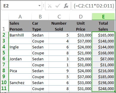
To see Total Sales of coupes and sedans for each salesperson, select cells E2:E11, enter the formula =C2:C11*D2:D11, and then press Ctrl+Shift+Enter.
To see the Grand Total of all sales, select cell F11, enter the formula =SUM(C2:C11*D2:D11), and then press Ctrl+Shift+Enter.

When you press Ctrl+Shift+Enter, Excel surrounds the formula with braces ({ }) and inserts an instance of the formula in each cell of the selected range. This happens very quickly, so what you see in column E is the total sales amount for each car type for each salesperson. If you select E2, then select E3, E4, and so on, you’ll see that the same formula is shown: {=C2:C11*D2:D11}.

Create a single-cell array formula

In cell D13 of the workbook, type the following formula, and then press Ctrl+Shift+Enter:

=SUM(C2:C11*D2:D11)

In this case, Excel multiplies the values in the array (the cell range C2 through D11) and then uses the SUM function to add the totals together. The result is a grand total of $1,590,000 in sales. This example shows how powerful this type of formula can be. For example, suppose you have 1,000 rows of data. You can sum part or all of that data by creating an array formula in a single cell instead of dragging the formula down through the 1,000 rows.

Also, notice that the single-cell formula in cell D13 is completely independent of the multi-cell formula (the formula in cells E2 through E11). This is another advantage of using array formulas — flexibility. You could change the formulas in column E or delete that column altogether, without affecting the formula in D13.

Array formulas also offer these advantages:

Consistency If you click any of the cells from E2 downward, you see the same formula. That consistency can help ensure greater accuracy.
Safety You cannot overwrite a component of a multi-cell array formula. For example, click cell E3 and press Delete. You have to either select the entire range of cells (E2 through E11) and change the formula for the entire array, or leave the array as is. As an added safety measure, you have to press Ctrl+Shift+Enter to confirm any change to the formula.
Smaller file sizes You can often use a single array formula instead of several intermediate formulas. For example, the workbook uses one array formula to calculate the results in column E. If you had used standard formulas (such as =C2*D2, C3*D3, C4*D4…), you would have used 11 different formulas to calculate the same results.

In general, array formulas use standard formula syntax. They all begin with an equal (=) sign, and you can use most of the built-in Excel functions in your array formulas. The key difference is that when using an array formula, you press Ctrl+Shift+Enter to enter your formula. When you do this, Excel surrounds your array formula with braces — if you type the braces manually, your formula will be converted to a text string, and it won’t work.

Array functions can be an efficient way to build complex formulas. The array formula =SUM(C2:C11*D2:D11) is the same as this: =SUM(C2*D2,C3*D3,C4*D4,C5*D5,C6*D6,C7*D7,C8*D8,C9*D9,C10*D10,C11*D11).

Important: Press Ctrl+Shift+Enter whenever you need to enter an array formula. This applies to both single-cell and multi-cell formulas.

Whenever you work with multi-cell formulas, also remember:

Select the range of cells to hold your results before you enter the formula. You did this when you created the multi-cell array formula when you selected cells E2 through E11.
You can’t change the contents of an individual cell in an array formula. To try this, select cell E3 in the workbook and press Delete. Excel displays a message that tells you that you can’t change part of an array.
You can move or delete an entire array formula, but you can’t move or delete part of it. In other words, to shrink an array formula, you first delete the existing formula and then start over.
To delete an array formula, select the entire formula range (for example, E2:E11), then press Delete.
You can’t insert blank cells into, or delete cells from a multi-cell array formula.

At times, you may need to expand an array formula. Select the first cell in existing array range, and continue until you’ve selected the entire range that you want to extend the formula to. Press F2 to edit the formula, then press CTRL+SHIFT+ENTER to confirm the formula once you’ve adjusted the formula range. The key is to select the entire range, starting with the top-left cell in the array. The top-left cell is the one that gets edited.

Array formulas are great, but they can have some disadvantages:

You may occasionally forget to press Ctrl+Shift+Enter. It can happen to even the most experienced Excel users. Remember to press this key combination whenever you enter or edit an array formula.
Other users of your workbook might not understand your formulas. In practice, array formulas are generally not explained in a worksheet. Therefore, if other people need to modify your workbooks, you should either avoid array formulas or make sure those people know about any array formulas and understand how to change them, if they need to.
Depending on the processing speed and memory of your computer, large array formulas can slow down calculations.

Array constants are a component of array formulas. You create array constants by entering a list of items and then manually surrounding the list with braces ({ }), like this:

={1,2,3,4,5}

By now, you know you need to press Ctrl+Shift+Enter when you create array formulas. Because array constants are a component of array formulas, you surround the constants with braces by manually typing them. You then use Ctrl+Shift+Enter to enter the entire formula.

Here’s an array in a single row: {1,2,3,4}. Here’s an array in a single column: {1;2;3;4}. And here’s an array of two rows and four columns: {1,2,3,4;5,6,7,8}. In the two row array, the first row is 1, 2, 3, and 4, and the second row is 5, 6, 7, and 8. A single semicolon separates the two rows, between 4 and 5.

As with array formulas, you can use array constants with most of the built-in functions that Excel provides. The following sections explain how to create each kind of constant and how to use these constants with functions in Excel.

The following procedures will give you some practice in creating horizontal, vertical, and two-dimensional constants.

Create a horizontal constant

In a blank worksheet, select cells A1 through E1.
In the formula bar, enter the following formula, and then press Ctrl+Shift+Enter:

={1,2,3,4,5}

In this case, you should type the opening and closing braces ({ }), and Excel will add the second set for you.

The following result is displayed.

Create a vertical constant

In your workbook, select a column of five cells.
In the formula bar, enter the following formula, and then press Ctrl+Shift+Enter:

={1;2;3;4;5}

The following result is displayed.

Create a two-dimensional constant

In your workbook, select a block of cells four columns wide by three rows high.
In the formula bar, enter the following formula, and then press Ctrl+Shift+Enter:

={1,2,3,4;5,6,7,8;9,10,11,12}

You see the following result:

Use constants in formulas

Here is a simple example that uses constants:

In the sample workbook, create a new worksheet.
In cell A1, type 3, and then type 4 in B1, 5 in C1, 6 in D1, and 7 in E1.
In cell A3, type the following formula, and then press Ctrl+Shift+Enter:

=SUM(A1:E1*{1,2,3,4,5})

Notice that Excel surrounds the constant with another set of braces, because you entered it as an array formula.

The value 85 appears in cell A3.

The next section explains how the formula works.

The formula you just used contains several parts.

1. Function

2. Stored array

3. Operator

4. Array constant

The last element inside the parentheses is the array constant: {1,2,3,4,5}. Remember that Excel does not surround array constants with braces; you actually type them. Also remember that after you add a constant to an array formula, you press Ctrl+Shift+Enter to enter the formula.

Because Excel performs operations on expressions enclosed in parentheses first, the next two elements that come into play are the values stored in the workbook (A1:E1) and the operator. At this point, the formula multiplies the values in the stored array by the corresponding values in the constant. It’s the equivalent of:

=SUM(A1*1,B1*2,C1*3,D1*4,E1*5)

Finally, the SUM function adds the values, and the sum 85 appears in cell A3.

To avoid using the stored array and to just keep the operation entirely in memory, replace the stored array with another array constant:

=SUM({3,4,5,6,7}*{1,2,3,4,5})

To try this, copy the function, select a blank cell in your workbook, paste the formula into the formula bar, and then press Ctrl+Shift+Enter. You’ll see the same result as you did in the earlier exercise that used the array formula:

=SUM(A1:E1*{1,2,3,4,5})

Array constants can contain numbers, text, logical values (such as TRUE and FALSE), and error values ( such as #N/A). You can use numbers in the integer, decimal, and scientific formats. If you include text, you need to surround the text with quotation marks («).

Array constants can’t contain additional arrays, formulas, or functions. In other words, they can contain only text or numbers that are separated by commas or semicolons. Excel displays a warning message when you enter a formula such as {1,2,A1:D4} or {1,2,SUM(Q2:Z8)}. Also, numeric values can’t contain percent signs, dollar signs, commas, or parentheses.

One of the best way to use array constants is to name them. Named constants can be much easier to use, and they can hide some of the complexity of your array formulas from others. To name an array constant and use it in a formula, do the following:

On the Formulas tab, in the Defined Names group, click Define Name.
The Define Name dialog box appears.
In the Name box, type Quarter1.
In the Refers to box, enter the following constant (remember to type the braces manually):

={«January»,»February»,»March»}

The contents of the dialog box now looks like this:
Click OK, and then select a row of three blank cells.
Type the following formula, and then press Ctrl+Shift+Enter.

=Quarter1

The following result is displayed.

When you use a named constant as an array formula, remember to enter the equal sign. If you don’t, Excel interprets the array as a string of text and your formula won’t work as expected. Finally, keep in mind that you can use combinations of text and numbers.

Look for the following problems when your array constants don’t work:

Some elements might not be separated with the proper character. If you omit a comma or semicolon, or if you put one in the wrong place, the array constant might not be created correctly, or you might see a warning message.
You might have selected a range of cells that doesn’t match the number of elements in your constant. For example, if you select a column of six cells for use with a five-cell constant, the #N/A error value appears in the empty cell. Conversely, if you select too few cells, Excel omits the values that don’t have a corresponding cell.

Multiply each item in an array

Create a new worksheet, and then select a block of empty cells four columns wide by three rows high.
Type the following formula, and then press Ctrl+Shift+Enter:

={1,2,3,4;5,6,7,8;9,10,11,12}*2

Square the items in an array

Select a block of empty cells four columns wide by three rows high.
Type the following array formula, and then press Ctrl+Shift+Enter:

={1,2,3,4;5,6,7,8;9,10,11,12}*{1,2,3,4;5,6,7,8;9,10,11,12}

Alternatively, enter this array formula, which uses the caret operator (^):

={1,2,3,4;5,6,7,8;9,10,11,12}^2

Transpose a one-dimensional row

Select a column of five blank cells.
Type the following formula, and then press Ctrl+Shift+Enter:

=TRANSPOSE({1,2,3,4,5})

Even though you entered a horizontal array constant, the TRANSPOSE function converts the array constant into a column.

Transpose a one-dimensional column

Select a row of five blank cells.
Enter the following formula, and then press Ctrl+Shift+Enter:

=TRANSPOSE({1;2;3;4;5})

Even though you entered a vertical array constant, the TRANSPOSE function converts the constant into a row.

Transpose a two-dimensional constant

Select a block of cells three columns wide by four rows high.
Enter the following constant, and then press Ctrl+Shift+Enter:

=TRANSPOSE({1,2,3,4;5,6,7,8;9,10,11,12})

The TRANSPOSE function converts each row into a series of columns.

This section provides examples of basic array formulas.

Create arrays and array constants from existing values

The following example explains how to use array formulas to create links between ranges of cells in different worksheets. It also shows you how to create an array constant from the same set of values.

Create an array from existing values

On a worksheet in Excel, select cells C8:E10, and enter this formula:

={10,20,30;40,50,60;70,80,90}

Be sure to type { (opening brace) before you type 10, and } (closing brace) after you type 90, because you’re creating an array of numbers.
Press Ctrl+Shift+Enter, which enters this array of numbers in the cell range C8:E10 by using an array formula. On your worksheet, C8 through E10 should look like this:

10

20

30

40

50

60

70

80

90
Select the cell range C1 through E3.
Enter the following formula in the formula bar, and then press Ctrl+Shift+Enter:

=C8:E10

A 3×3 array of cells appears in cells C1 through E3 with the same values you see in C8 through E10.

10	20	30
40	50	60
70	80	90

Create an array constant from existing values

With cells C1:C3 selected, press F2 to switch to edit mode.
Press F9 to convert the cell references to values. Excel converts the values into an array constant. The formula should now be ={10,20,30;40,50,60;70,80,90}.
Press Ctrl+Shift+Enter to enter the array constant as an array formula.

Count characters in a range of cells

The following example shows you how to count the number of characters, including spaces, in a range of cells.

Copy this entire table and paste into a worksheet in cell A1.

Data
This is a
bunch of cells that
come together
to form a
single sentence.

Total characters in A2:A6
=SUM(LEN(A2:A6))

Contents of longest cell (A3)
=INDEX(A2:A6,MATCH(MAX(LEN(A2:A6)),LEN(A2:A6),0),1)

Select cell A8, and then press Ctrl+Shift+Enter to see the total number of characters in cells A2:A6 (66).
Select cell A10, and then press Ctrl+Shift+Enter to see the contents of the longest of cells A2:A6 (cell A3).

The following formula is used in cell A8 counts the total number of characters (66) in cells A2 through A6.

=SUM(LEN(A2:A6))

In this case, the LEN function returns the length of each text string in each of the cells in the range. The SUM function then adds those values together and displays the result (66).

Find the n smallest values in a range

This example shows how to find the three smallest values in a range of cells.

Enter some random numbers in cells A1:A11.
Select cells C1 through C3. This set of cells will hold the results returned by the array formula.
Enter the following formula, and then press Ctrl+Shift+Enter:

=SMALL(A1:A11,{1;2;3})

This formula uses an array constant to evaluate the SMALL function three times and return the smallest (1), second smallest (2), and third smallest (3) members in the array that is contained in cells A1:A10 To find more values, you add more arguments to the constant. You can also use additional functions with this formula, such as SUM or AVERAGE. For example:

=SUM(SMALL(A1:A10,{1,2,3})

=AVERAGE(SMALL(A1:A10,{1,2,3})

Find the n largest values in a range

To find the largest values in a range, you can replace the SMALL function with the LARGE function. In addition, the following example uses the ROW and INDIRECT functions.

Select cells D1 through D3.
In the formula bar, enter this formula, and then press Ctrl+Shift+Enter:

=LARGE(A1:A10,ROW(INDIRECT(«1:3»)))

At this point, it may help to know a bit about the ROW and INDIRECT functions. You can use the ROW function to create an array of consecutive integers. For example, select an empty column of 10 cells in your practice workbook, enter this array formula, and then press Ctrl+Shift+Enter:

=ROW(1:10)

The formula creates a column of 10 consecutive integers. To see a potential problem, insert a row above the range that contains the array formula (that is, above row 1). Excel adjusts the row references, and the formula generates integers from 2 to 11. To fix that problem, you add the INDIRECT function to the formula:

=ROW(INDIRECT(«1:10»))

The INDIRECT function uses text strings as its arguments (which is why the range 1:10 is surrounded by double quotation marks). Excel does not adjust text values when you insert rows or otherwise move the array formula. As a result, the ROW function always generates the array of integers that you want.

Let’s take a look at the formula that you used earlier — =LARGE(A5:A14,ROW(INDIRECT(«1:3»))) — starting from the inner parentheses and working outward: The INDIRECT function returns a set of text values, in this case the values 1 through 3. The ROW function in turn generates a three-cell columnar array. The LARGE function uses the values in the cell range A5:A14, and it is evaluated three times, once for each reference returned by the ROW function. The values 3200, 2700, and 2000 are returned to the three-cell columnar array. If you want to find more values, you add a greater cell range to the INDIRECT function.

As with earlier examples, you can use this formula with other functions, such as SUM and AVERAGE.

Find the longest text string in a range of cells

Go back to the earlier text string example, enter the following formula in an empty cell, and press Ctrl+Shift+Enter:

=INDEX(A2:A6,MATCH(MAX(LEN(A2:A6)),LEN(A2:A6),0),1)

The text «bunch of cells that» appears.

Let’s take a closer look at the formula, starting from the inner elements and working outward. The LEN function returns the length of each of the items in the cell range A2:A6. The MAX function calculates the largest value among those items, which corresponds to the longest text string, which is in cell A3.

Here’s where things get a little complex. The MATCH function calculates the offset (the relative position) of the cell that contains the longest text string. To do that, it requires three arguments: a lookup value, a lookup array, and a match type. The MATCH function searches the lookup array for the specified lookup value. In this case, the lookup value is the longest text string:

(MAX(LEN(A2:A6))

and that string resides in this array:

LEN(A2:A6)

The match type argument is 0. The match type can consist of a 1, 0, or -1 value. If you specify 1, MATCH returns the largest value that is less than or equal to the lookup value. If you specify 0, MATCH returns the first value exactly equal to the lookup value. If you specify -1, MATCH finds the smallest value that is greater than or equal to the specified lookup value. If you omit a match type, Excel assumes 1.

Finally, the INDEX function takes these arguments: an array, and a row and column number within that array. The cell range A2:A6 provides the array, the MATCH function provides the cell address, and the final argument (1) specifies that the value comes from the first column in the array.

This section provides examples of advanced array formulas.

Sum a range that contains error values

The SUM function in Excel does not work when you try to sum a range that contains an error value, such as #N/A. This example shows you how to sum the values in a range named Data that contains errors.

=SUM(IF(ISERROR(Data),»»,Data))

The formula creates a new array that contains the original values minus any error values. Starting from the inner functions and working outward, the ISERROR function searches the cell range (Data) for errors. The IF function returns a specific value if a condition you specify evaluates to TRUE and another value if it evaluates to FALSE. In this case, it returns empty strings («») for all error values because they evaluate to TRUE, and it returns the remaining values from the range (Data) because they evaluate to FALSE, meaning that they don’t contain error values. The SUM function then calculates the total for the filtered array.

Count the number of error values in a range

This example is similar to the previous formula, but it returns the number of error values in a range named Data instead of filtering them out:

=SUM(IF(ISERROR(Data),1,0))

This formula creates an array that contains the value 1 for the cells that contain errors and the value 0 for the cells that don’t contain errors. You can simplify the formula and achieve the same result by removing the third argument for the IF function, like this:

=SUM(IF(ISERROR(Data),1))

If you don’t specify the argument, the IF function returns FALSE if a cell does not contain an error value. You can simplify the formula even more:

=SUM(IF(ISERROR(Data)*1))

This version works because TRUE*1=1 and FALSE*1=0.

Sum values based on conditions

You might need to sum values based on conditions. For example, this array formula sums just the positive integers in a range named Sales:

=SUM(IF(Sales>0,Sales))

The IF function creates an array of positive values and false values. The SUM function essentially ignores the false values because 0+0=0. The cell range that you use in this formula can consist of any number of rows and columns.

You can also sum values that meet more than one condition. For example, this array formula calculates values greater than 0 and less than or equal to 5:

=SUM((Sales>0)*(Sales<=5)*(Sales))

Keep in mind that this formula returns an error if the range contains one or more non-numeric cells.

You can also create array formulas that use a type of OR condition. For example, you can sum values that are less than 5 and greater than 15:

=SUM(IF((Sales<5)+(Sales>15),Sales))

The IF function finds all values smaller than 5 and greater than 15 and then passes those values to the SUM function.

You can’t use the AND and OR functions in array formulas directly because those functions return a single result, either TRUE or FALSE, and array functions require arrays of results. You can work around the problem by using the logic shown in the previous formula. In other words, you perform math operations, such as addition or multiplication, on values that meet the OR or AND condition.

Compute an average that excludes zeros

This example shows you how to remove zeros from a range when you need to average the values in that range. The formula uses a data range named Sales:

=AVERAGE(IF(Sales<>0,Sales))

The IF function creates an array of values that do not equal 0 and then passes those values to the AVERAGE function.

Count the number of differences between two ranges of cells

This array formula compares the values in two ranges of cells named MyData and YourData and returns the number of differences between the two. If the contents of the two ranges are identical, the formula returns 0. To use this formula, the cell ranges need to be the same size and of the same dimension (for example, if MyData is a range of 3 rows by 5 columns, YourData must also be 3 rows by 5 columns):

=SUM(IF(MyData=YourData,0,1))

The formula creates a new array of the same size as the ranges that you are comparing. The IF function fills the array with the value 0 and the value 1 (0 for mismatches and 1 for identical cells). The SUM function then returns the sum of the values in the array.

You can simplify the formula like this:

=SUM(1*(MyData<>YourData))

Like the formula that counts error values in a range, this formula works because TRUE*1=1, and FALSE*1=0.

Find the location of the maximum value in a range

This array formula returns the row number of the maximum value in a single-column range named Data:

=MIN(IF(Data=MAX(Data),ROW(Data),»»))

The IF function creates a new array that corresponds to the range named Data. If a corresponding cell contains the maximum value in the range, the array contains the row number. Otherwise, the array contains an empty string («»). The MIN function uses the new array as its second argument and returns the smallest value, which corresponds to the row number of the maximum value in Data. If the range named Data contains identical maximum values, the formula returns the row of the first value.

If you want to return the actual cell address of a maximum value, use this formula:

=ADDRESS(MIN(IF(Data=MAX(Data),ROW(Data),»»)),COLUMN(Data))

Acknowledgement

Parts of this article were based on a series of Excel Power User columns written by Colin Wilcox, and adapted from chapters 14 and 15 of Excel 2002 Formulas, a book written by John Walkenbach, a former Excel MVP.

Need more help?

You can always ask an expert in the Excel Tech Community or get support in the Answers community.

Функция Array

Возвращает значение Variant, содержащее массив.

Синтаксис

Array(arglist)

Обязательный аргументarglist представляет собой разделенный запятыми список значений, назначенных элементам массива, содержащимся в Variant. Если аргументы не указаны, создается пустой массив.

Примечания

Эта нотация, используемая для ссылки на элемент массива, состоит из имени переменной, за которой в скобках содержится порядковый номер, указывающий нужный элемент.

В приведенном ниже примере первый оператор создает переменную с именем A как переменную типа Variant. Второй оператор назначает массив переменной A . Последний оператор присваивает значение, содержащееся во втором элементе массива, другой переменной.

Нижняя граница массива, создаваемого с помощью функции Array, определяется нижней границей, указанной в операторе Option Base, кроме случаев, когда к Array добавляется имя библиотеки типов (например, VBA.Array). Если имя библиотеки типов добавлено, оператор Option Base не влияет на функцию Array.

Переменная Variant, не объявленная как массив, также может содержать массив. Переменная Variant может содержать массив любого типа, за исключением строк фиксированной длины и пользовательских типов. Хотя переменная Variant, содержащая массив, по существу отличается от массива, элементы которого имеют тип Variant, доступ к элементам массива осуществляется так же.

Пример

В данном примере функция Array возвращает переменную Variant, содержащую массив.

См. также

Поддержка и обратная связь

Есть вопросы или отзывы, касающиеся Office VBA или этой статьи? Руководство по другим способам получения поддержки и отправки отзывов см. в статье Поддержка Office VBA и обратная связь.

Источник

What is an array formula?

Summary

In the world of Excel formulas, the term «array formula» is probably responsible for more confusion than just about any other concept. This is because the definition of an array formula has become mixed up with the requirement to enter some array formulas in a special way, with control + shift + enter.

Introduction

What is an array formula anyway?

In simple terms, an array formula is a formula that works with an array of values, rather than a single value. Array formulas can return a single result, or multiple results.

That sounds simple enough, and indeed many array formulas are not complex. However, because some array formulas need to be entered in a special way, and some don’t, array formulas live mostly in the geeky realm of super users.

In fact, in the world of Excel formulas, the term «array formula» may be responsible for more confusion than just about any other concept.

With the introduction of Dynamic Arrays in Excel 365, array formulas are going to become a lot more common, because they are now much easier to use and understand:

No need for control + shift + enter
Formulas that return multiple results will spill

We’ve been working on a new course, Dynamic Array formulas, and these videos help explain the topics discussed below:

Basic array formula example

In the example below, we want to find the maximum change in temperature over seven days:

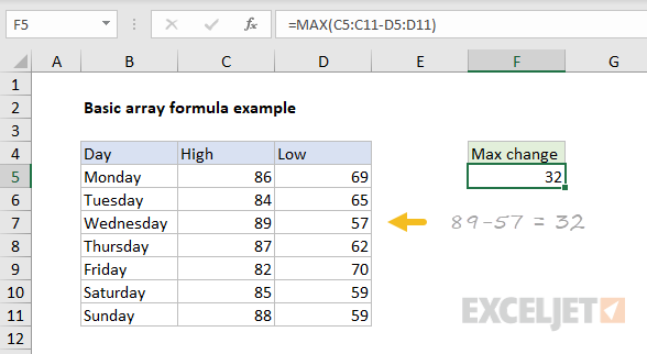
The formula in F5 is:

This is an array formula that returns a single result.

Working from the inside out, we first subtract the low temps from high temps:

Each range contains 7 values, which we can expand into arrays like this:

This is called an array operation. We are working with multiple values, and the result after subtraction is a new array with 7 values, where each value represents the change in temperature on the given day:

The new array is returned directly to the MAX function which returns the largest value:

You can see that this array formula is actually quite simple!

Traditional Excel — complication and danger

The problem arises when we enter the formula. In «Traditional Excel» (currently, every version of Excel except Office 365), this formula must be entered with control + shift + enter. When entered this way, Excel will display curly braces in the formula bar like this:

These curly braces tell you that Excel is handling the formula as an array formula. In other words, Excel is «letting you» work with multiple values.

To most users, that’s pretty strange and confusing. But it gets worse.

If you (or someone else) forgets to enter the formula with control + shift + enter, the same exact formula may return an incorrect result.

For example, the formula above without control + shift + enter will return 17, the change in temperature on Monday. This will be a «silent failure» – no warning will occur. The formula will simply stop working correctly.

Obviously, formulas that return incorrect results are bad news 🙂

Dynamic Excel — simplicity and clarity

The great thing about the Dynamic Array version of Excel, is that array formulas just work. You don’t have to use control + shift + enter with any array formula.

Even better, a formula that returns multiple multiple values will spill these values onto the worksheet. This makes array formulas much easier to understand, because it’s obvious when a formula is returning more than one value.

In contrast, the same formulas in previous versions of Excel will display only one result in a single cell, no matter how many values are actually returned.

The bottom line is that working with array formulas in Excel is now easier and more intuitive than ever. You can now use array formulas whenever you like, without worrying about fancy syntax requirements.

Источник

Create an array formula

Array formulas are powerful formulas that enable you to perform complex calculations that often can’t be done with standard worksheet functions. They are also referred to as «Ctrl-Shift-Enter» or «CSE» formulas, because you need to press Ctrl+Shift+Enter to enter them. You can use array formulas to do the seemingly impossible, such as

Count the number of characters in a range of cells.

Sum numbers that meet certain conditions, such as the lowest values in a range or numbers that fall between an upper and lower boundary.

Sum every nth value in a range of values.

Excel provides two types of array formulas: Array formulas that perform several calculations to generate a single result and array formulas that calculate multiple results. Some worksheet functions return arrays of values, or require an array of values as an argument. For more information, see Guidelines and examples of array formulas.

Note: If you have a current version of Microsoft 365, then you can simply enter the formula in the top-left-cell of the output range, then press ENTER to confirm the formula as a dynamic array formula. Otherwise, the formula must be entered as a legacy array formula by first selecting the output range, entering the formula in the top-left-cell of the output range, and then pressing CTRL+SHIFT+ENTER to confirm it. Excel inserts curly brackets at the beginning and end of the formula for you. For more information on array formulas, see Guidelines and examples of array formulas.

This type of array formula can simplify a worksheet model by replacing several different formulas with a single array formula.

Click the cell in which you want to enter the array formula.

Enter the formula that you want to use.

Array formulas use standard formula syntax. They all begin with an equal sign (=), and you can use any of the built-in Excel functions in your array formulas.

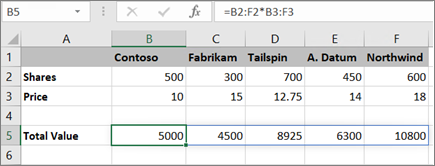
For example, this formula calculates the total value of an array of stock prices and shares, and places the result in the cell next to «Total Value.»

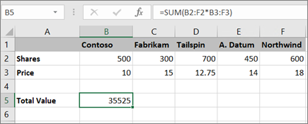
The formula first multiplies the shares (cells B2 – F2) by their prices (cells B3 – F3), and then adds those results to create a grand total of 35,525. This is an example of a single-cell array formula because the formula lives in just one cell.

Press Enter (if you have a current Microsoft 365 Subscription); otherwise press Ctrl+Shift+Enter.

When you press Ctrl+Shift+Enter, Excel automatically inserts the formula between (a pair of opening and closing braces).

To calculate multiple results by using an array formula, enter the array into a range of cells that has the exact same number of rows and columns that you’ll use in the array arguments.

Select the range of cells in which you want to enter the array formula.

Enter the formula that you want to use.

Array formulas use standard formula syntax. They all begin with an equal sign (=), and you can use any of the built-in Excel functions in your array formulas.

In the following example, the formula multiples shares by price in each column, and the formula lives in the selected cells in row 5.

Press Enter (if you have a current Microsoft 365 Subscription); otherwise press Ctrl+Shift+Enter.

When you press Ctrl+Shift+Enter, Excel automatically inserts the formula between (a pair of opening and closing braces).

If you need to include new data in your array formula, see Expand an array formula. You can also try:

Delete an array formula (you press Ctrl+Shift+Enter there, too)

Name an array constant (they can make constants easier to use)

Источник

Array formula

An array formula is a type of formula that performs an operation on multiple values instead of a single value. The final result of an array formula can be either one item or an array of items, depending on how the formula is constructed. For example, the following formula is an array formula that returns the sum of all characters in a range:

To work correctly, many (but not all) array formulas need to be entered with control + shift + enter. When you enter with control + shift + enter, you’ll see the formula wrapped in curly braces <> in the formula bar. Do not enter curly braces manually, or the formula won’t work.

What is an Array?

An array is a collection of more than one item. Arrays in Excel appear inside curly brackets. For example, <1;2;3>or <«red»,»blue»,»green»>. The reason arrays are so common in Excel is that they map directly to cell ranges. Vertical ranges are represented as arrays that use semicolons, for example <100;125;150>. Horizontal ranges are represented as arrays that use commas, for example <«small»,»medium»,»large»>. A two dimensional range will use both semicolons and commas.

Examples

Array formulas are somewhat difficult to understand, because the terminology is dense and complex. But array formulas themselves can be very simple. For example, this array formula tests the range A1:A5 for the value «a»:

The array operation is the comparison of each cell in A1:A5 to the string «a». Because the comparison operates on multiple values, it returns multiple results to the OR function:

If any item in the resultant array is TRUE, the OR function returns TRUE.

Sometimes array formulas supply multiple values as a function argument. For example, this array formula returns the total character count in the range B2:B11:

The LEN function is given multiple values in the range B2:B11 and returns multiple results in an array like this inside SUM:

where each item in the array represents the length of one cell value. The SUM function then sums all items and returns 43 as the final result.

Special syntax

In all versions of Excel except Excel 365, many array formulas need to be entered in a special way to work correctly. Instead of entering with the the «Enter» key, they need to be entered with Control + Shift + Enter. You’ll sometimes see Control + Shift + Enter abbreviated as «CSE», as in «CSE formula». A formula entered in this way will appear with curly braces on either side:

These braces are displayed automatically by Excel. Make sure you do not enter the curly braces manually!

Not all array formulas need to be entered with Control + Shift + Enter. Certain functions, like SUMPRODUCT, are programmed to handle array operations natively and usually don’t require Control + Shift + Enter. For example, both formulas below are array formulas that return the same result, but only the SUM version requires Control + Shift + Enter:

Excel 365

In Excel 365, array formula are native and do not require control + shift + enter. For a general introduction, see Dynamic Array Formulas in Excel.

Источник

Working with Excel array formula examples

The array of Excel functions allows you to solve complex tasks in automatically at the same time. We cannot complete the same tasks through the usual functions.

In fact, this is a group of functions that simultaneously process a group of data and immediately produce a result. Let’s consider in detail work with arrays of functions in Excel.

Types of Excel functions

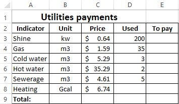
Array is a data grouped together. In this case, the group is an array of functions in Excel. Any table that we compose and fill in Excel can be called an array. Example:

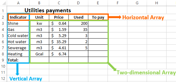
Depending on the location of the elements, the arrays are distinguished:

One-dimensional (data is in ONE line or in ONE column);
Two-dimensional (SEVERAL lines and columns, matrix).

One-dimensional arrays are:

Horizontal (data in a row);
Vertical (data in a column).

Note. Two-dimensional Excel arrays can take several sheets at once (these are hundreds and thousands of data).

Array formula allows you to process data from this array. It can return one value or result in an array (set) of values.

With the help of array formulas it is real to:

Count the number of characters in a certain range;
Summarize only those numbers that correspond to the given condition;
Summarize all n values in a certain range.

When we use array formulas, Excel takes into account the range of values not as individual cells, but as a single data block.

Array formulas syntax

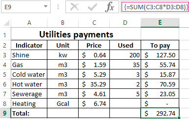
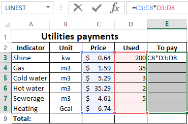
We use the formula of an array with a range of cells and with a separate cell. In the first case, we find the subtotals for the «To pay» «» column. In the second — the total amount of utility payments.

We select the range E3: E8.
Enter the following formula in the formula row: = C3: C8 * D3: D8.
Press the keys simultaneously: Ctrl + Shift + Enter. The subtotals are calculated:

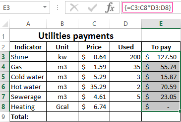
The formula after pressing Ctrl + Shift + Enter was in curly brackets. It was automatically inserted into each cell of the selected range.

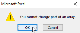
If you try to change the data in any cell in the «To pay» column, nothing happens. The formula in the array protects range values from changes. A corresponding entry appears on the screen:

Consider other examples of using the functions of an Excel array — calculate the total amount of utility payments using a single formula.

Select the cell E9 (opposite the «Total»).
We introduce a formula of the form:
Press the key combination: Ctrl + Shift + Enter. Result:

The formula of the array in this case replaced two simple formulas. This is a shortened version, which contains all the necessary information for solving a complex problem.

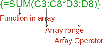
Arguments for a function are one-dimensional arrays. The formula looks at each of them individually, performs user-defined operations, and generates a single result.

Consider the syntax:

Working functions with Excel array

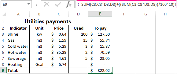
Let’s guess that it is planned to increase utility payments in 10% the next month. If we introduce the usual formula for the total is =SUM((C3:C8*D3:D8)+10%), then we are unlikely to get the expected result. We need each argument to increase in 10%. For the program to understand this, we use the function as an array.

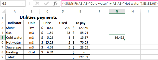
Let’s have a look how the «И» «AND» operator works in the array function. We need to find out how much we pay for the water, hot and cold. Function: The total is 86.46$.
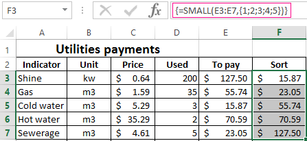
The Sort functions in the array formula. Sort the amounts to be paid in ascending order. For the sorted data list, create a range. Let’s select it (F3:F7). In the formula bar, we enter Press Ctrl + Shift + Enter.
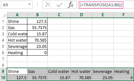
The transported matrix. There is a special Excel function for working with two-dimensional arrays. The «ТРАНСП» function returns several values at once. It converts a horizontal matrix to a vertical matrix and vice versa. Select the range of cells where the number of rows equals to the number of columns in the table with the original data. And the number of columns equals to the number of rows in the source array. Select range A9:F10. We introduce the formula: Press Ctrl + Shift + Enter. This results in an «inverted» data set.
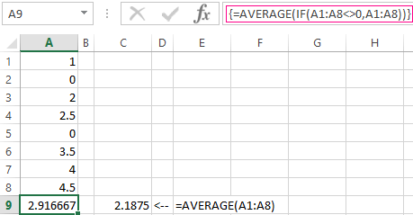
Search for the average without taking into account zeros. If we use the standard «AVERAGE» function, we get «0» as a result. And it will be correct. Therefore, we insert an additional condition into the formula:

0,A1:A8))’ >

A common mistake when working with arrays of functions is NOT to press the code combination «Ctrl + Shift + Enter» (never forget this key combination). This is the most important thing to remember when processing large amounts of information. Correctly entered function performs the most complicated tasks.

Источник

An array in Excel is a structure that holds a collection of values. Arrays can be mapped perfectly to ranges in a spreadsheet, which is why they are so important in Excel. An array can be thought of as a row of values, a column of values, or a combination of rows and columns with values. All cell references like A1:A5 and C1:F5 have underlying arrays, though the array structure is invisible in most contexts.

Example

In the example above, the three ranges map to arrays in a «row by column» scheme like this:

B5:D5 // 1 row x 3 columns
B8:B10 // 3 rows x 1 column
B13:D14  // 2 rows x 3 columns

If we display the values in these ranges as arrays, we have:

B5:D5={"red","green","blue"}
B8:B10={"red";"green";"blue"} 
B13:D14={10,20,30;40,50,60}

Notice arrays must represent a rectangular structure.

Array syntax

All arrays in Excel are wrapped in curly brackets {} and the delimiters between array elements indicate rows and/or columns. In the US version of Excel, a comma (,) separates columns and a semicolon (;) separates rows. For example, both arrays below contain numbers 1-3, but one is horizontal and one is vertical:

{1,2,3} // columns (horizontal)
{1;2;3} // rows (vertical)

Text values in an array appear in double quotes («») like this:

{"a","b","c"}

To «see» the array associated with a range, start a formula with an equal sign (=) and select the range. Then use the F9 key to inspect the underlying array. You can also use the ARRAYTOTEXT function to show how columns and rows are represented. Set format to 1 (strict) to see the complete array.

Delimiters in other languages

In other language versions of Excel, the delimiters for rows and column can vary. For example, the Spanish version of Excel uses a backslash () for columns and a semicolon (;) for rows:

{123} // columns
{1;2;3} // rows

Arrays in formulas

Since arrays map directly to ranges, all formulas work with arrays in some way, though it isn’t always obvious. A simple example is a formula that uses the SUM function to sum the range A1:A5, which contains 10,15,20,25,30. Inside SUM, the range resolves to an array of values. SUM then sums all values in the array and returns a single result of 100:

=SUM(A1:A5)
=SUM({10;15;20;25;30})
=100

Note: you can use the F9 key to «see» arrays in your Excel formulas. See this video for a demo on using F9 to debug.

Array formulas

Array formulas involve an operation that delivers an array of results. For example, here is a simple array formula that returns the total count of characters in the range A1:A5:

=SUM(LEN(A1:A5))

Inside the LEN function, A1:A5 is expanded to an array of values. The LEN function then generates a character count for each value and returns an array of 5 results. The SUM function then returns the sum of all items in the array.

Dynamic arrays

With the introduction of Dynamic Array formulas in Excel, arrays have become more important, since it is easier than ever to write formulas that work with multiple results at the same time.

Источник

The array of Excel functions allows you to solve complex tasks in automatically at the same time. We cannot complete the same tasks through the usual functions.

In fact, this is a group of functions that simultaneously process a group of data and immediately produce a result. Let’s consider in detail work with arrays of functions in Excel.

Types of Excel functions

Array is a data grouped together. In this case, the group is an array of functions in Excel. Any table that we compose and fill in Excel can be called an array. Example:

Depending on the location of the elements, the arrays are distinguished:

One-dimensional (data is in ONE line or in ONE column);
Two-dimensional (SEVERAL lines and columns, matrix).

One-dimensional arrays are:

Horizontal (data in a row);
Vertical (data in a column).

Note. Two-dimensional Excel arrays can take several sheets at once (these are hundreds and thousands of data).

Array formula allows you to process data from this array. It can return one value or result in an array (set) of values.

With the help of array formulas it is real to:

Count the number of characters in a certain range;
Summarize only those numbers that correspond to the given condition;
Summarize all n values in a certain range.

When we use array formulas, Excel takes into account the range of values not as individual cells, but as a single data block.

Array formulas syntax

We select the range E3: E8.
Enter the following formula in the formula row: = C3: C8 * D3: D8.

Press the keys simultaneously: Ctrl + Shift + Enter. The subtotals are calculated:

The formula after pressing Ctrl + Shift + Enter was in curly brackets. It was automatically inserted into each cell of the selected range.

If you try to change the data in any cell in the «To pay» column, nothing happens. The formula in the array protects range values from changes. A corresponding entry appears on the screen:

To pay.

Consider other examples of using the functions of an Excel array — calculate the total amount of utility payments using a single formula.

Select the cell E9 (opposite the «Total»).
We introduce a formula of the form:
Press the key combination: Ctrl + Shift + Enter. Result:

The formula of the array in this case replaced two simple formulas. This is a shortened version, which contains all the necessary information for solving a complex problem.

Arguments for a function are one-dimensional arrays. The formula looks at each of them individually, performs user-defined operations, and generates a single result.

Consider the syntax:

Working functions with Excel array

Let’s have a look how the «И» «AND» operator works in the array function. We need to find out how much we pay for the water, hot and cold. Function:
The total is 86.46$.

The Sort functions in the array formula. Sort the amounts to be paid in ascending order. For the sorted data list, create a range. Let’s select it (F3:F7). In the formula bar, we enter
Press Ctrl + Shift + Enter.

The transported matrix. There is a special Excel function for working with two-dimensional arrays. The «ТРАНСП» function returns several values at once. It converts a horizontal matrix to a vertical matrix and vice versa. Select the range of cells where the number of rows equals to the number of columns in the table with the original data. And the number of columns equals to the number of rows in the source array. Select range A9:F10. We introduce the formula:
Press Ctrl + Shift + Enter. This results in an «inverted» data set.

Search for the average without taking into account zeros. If we use the standard «AVERAGE» function, we get «0» as a result. And it will be correct. Therefore, we insert an additional condition into the formula:

We get:

Download array formula examples

Источник

Array formulas are very useful and powerful formulas used to perform some of the very complex calculations in Excel. It is also known as the CSE formula. We need to press “CTRL + SHIFT + ENTER” together to execute array formulas instead of pressing enter. There are two types of array formulas: one that gives us a single result and another that provides multiple results.

For example, suppose you have the data set showing the production and cost for the four products, and you need to calculate the total cost of all the products. We could do this by simply adding formula in the column that multiplies the production and costs of the products and then adding a sum at the bottom of the column. However, the array formulas avoid these steps and provide an answer with a single formula.

Arrays in excelA VBA array in excel is a storage unit or a variable which can store multiple data values. These values must necessarily be of the same data type. This implies that the related values are grouped together to be stored in an array variable.read more can be termed array formulas in Excel. Array in Excel is a powerful formula that enables us to perform complex calculations.

What is an Array? An array is a set of values or variables in a data set like {a,b,c,d} is an array that has values from “a” to “d.” Similarly, in an Excel array is a range of cells of values,

In the above screenshot, cells from B2 to cell G2 are an array or range of cells.

These are also known as “CSE formulas” or “Control Shift Enter Formulas.” For example, for creating an array formula in Excel, we must press “Ctrl + Shift + Enter.”

In Excel, we have two types of array formulas:

One, which gives us a single result.
Another which gives us more than one result.

We will learn both the types of array formulas on this topic.

Array Formulas in Excel
- Explanation of Array Formulas in Excel
- How to Use Array Formulas in Excel?
- Example #1
- Example #2
- Example #3
- Things to Remember
- Recommended Articles

Explanation of Array Formulas in Excel

Array formulas in Excel are powerful formulas that help us perform very complex calculations.

We learned from the above examples that these formulas in Excel simplify complex and lengthy calculations. There is one thing to remember. However, in example 2, we returned multiple values using these formulas in Excel. We cannot change or cut the cell’s value as it is a part of an array.

Suppose we want to delete cell G6 Excel. It will give us an error. Even if we change the value in the cell type, any random value in the cell Excel will provide an error.

For example, type a number in cell G6 and press the “Enter” key. It may provide the following error,

Upon typing a random value 56 in cell G6, it may give an error that we cannot change a part of the array.

If we need to edit an array formula, go to the function bar and edit the provided values or range. If we want to delete the array formula, delete the whole array, i.e., cell range B6 to G6.

How to Use Array Formulas in Excel?

Let us learn an array formula by a few examples:

You can download this Array Formula Excel Template here – Array Formula Excel Template

One can use array formulas in two types:

If we want to return a single value, use these formulas in a single cell, as in example 1.
If we want to return more than one value, use these formulas in Excel by selecting the range of cells as in example 2.
Press CTRL + Shift + Enter to make an array formula.

Example #1

A restaurant’s sales data consists of each product’s price and the number of products sold.

The owner wants to calculate the total sales done by those products.

The owner multiplies the number of items sold for each product then sums them up as in the given-below equation,

Also, he gets the total sales as given below:

But this is a lengthy task. If the data were bigger, it would be much more tedious. So instead, Excel offers array of formulas for such tasks.

We will create our first array formula in cell B7.

The following are the steps to make the first array: –

In cell B7, type =SUM and press the “tab” button on the keyboard. It may open up the sum formula.
Select the cell range from B2 to G2.
Now, put an asterisk “*” sign after B2:G2 to multiply.
Select the cell range from B3 to G3.
Instead of pressing the “Enter” key, press “CTRL + SHIFT + ENTER.”

As a result, Excel may provide the total sales value by multiplying the number of products by the price in each column and summing them up. For example, in the highlighted section, we can see that Excel has created an array for cell range B2 to G2 and B3 to G3.

The above example explains how Excel array formulas return a single value for an array or set of data.

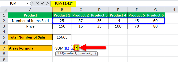
Example #2

With the same data, what if the owner wants to know the sales for each product separately, like sales of products 1 and 2?

He can either go a long way. In each cell, perform a function that will calculate the sales value.

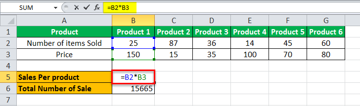
The equation mentioned in cell B5 will be required to repeat for cells C4, D4, etc.

Again, it would be a tedious task if it were larger data.

In this example, we will learn how array formulas in Excel return multiple values for a set of arrays.

#1 – Select the cells where we want our subtotals, i.e., per product sales for each product. In this case, it is a cell range B8 to G8.

#2 – Type an equal to sign “=” a

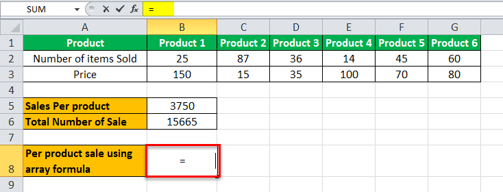
#3 –Select cell range B2 to G2.

#4 – Type an asterisk “*” sign after B2:G2.

#5 – Now, select cell range B3 to G3.

#6 – Do not press the “Enter” key for the array formula. Press “CTRL + SHIFT + ENTER” for array formula.

The above example explains how an array formula can return multiple values for an array in Excel.

Cells B6 to G6 are an array.

Example #3

For the same restaurant owner, he has the restaurant sales data for six months Jan, Feb, March, April, May, and June. He wants to know the average growth rate for sales.

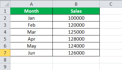
The owner can normally subtract the sales value of Feb month to Jan in cell C2 and then calculate the average.

Again, it would be a tiresome task if this were larger data. So let us do this with the array in Excel formulas.

#1 – In cell D8, type =average. Then, press the “tab” button.

#2 – To calculate growth, we will need to subtract the values of one month from the previous month to select the cell range from B3 to B7.

#3 – Put a subtract (-) sign after B3:B7,

#4 – Now, select cells from B2 to B6.

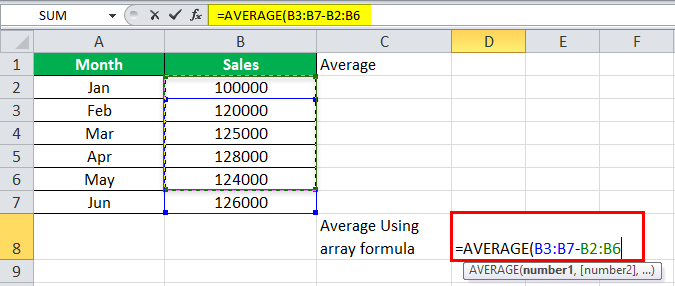
#5 – As for the array in Excel, do not press the “Enter” key. Press “CTRL + SHIFT + ENTER.”

Array formulas in Excel easily calculated the average growth for the sales without any hassle.

The owner now does not require calculating each month’s growth and performs the average function after that.

Things to Remember

These are also known as CSE Formulas or Control Shift Enter ExcelCtrl-Shift Enter In Excel is a shortcut command that facilitates implementing the array formula in the excel function to execute an intricate computation of the given data. Altogether it transforms a particular data into an array format in excel with multiple data values for this purpose.read more Formulas.
Do not make parenthesis for an array; Excel itself does that. It would return an error or incorrect value.
Entering the parenthesis “{“manually, Excel will treat it as a text.
Do not press the “Enter” key. Instead, press “CTRL + SHIFT + Enter” to use an array formula.
We cannot change the cell of an array. So, to modify an array formula, either modify the formula from the function bar or delete the formula and redesign it in the desired format.

Download our examples

Acknowledgement

Need more help?

See Also

Функция Array

Синтаксис

Примечания

Пример

См. также

Поддержка и обратная связь

What is an array formula?

Summary

Introduction

Basic array formula example

Traditional Excel — complication and danger

Dynamic Excel — simplicity and clarity

Create an array formula

Array formula

What is an Array?

Examples

Special syntax

Excel 365

Working with Excel array formula examples

Types of Excel functions

Array formulas syntax

Working functions with Excel array

Example

Array syntax

Delimiters in other languages

Arrays in formulas

Array formulas

Dynamic arrays

Types of Excel functions

Array formulas syntax

Working functions with Excel array

Table of contents

Explanation of Array Formulas in Excel

How to Use Array Formulas in Excel?

Example #1

Example #2

Example #3

Things to Remember

Recommended Articles