
What is ANOVA in Excel?
ANOVA in Excel is a built-in statistical test used to analyze the variances. For example, we usually compare the available alternatives when buying a new item, which eventually helps us choose the best from all the available options. Using the ANOVA test in Excel can help us test the different data sets against each other to identify the best from the lot.
Assume you conducted a survey on three different flavors of ice creams, and you have collated opinions from users. Now, you need to identify which flavor is best among the views. Here, we have three different flavors of ice creams. These are called alternatives, so we can locate the best from the lot by running the ANOVA test in Excel.
You are free to use this image on your website, templates, etc, Please provide us with an attribution linkArticle Link to be Hyperlinked
For eg:
Source: ANOVA in Excel (wallstreetmojo.com)
Table of contents
- What is ANOVA in Excel?
- Where is ANOVA in Excel?
- How to do ANOVA Test in Excel?
- Things to Remember
- Recommended Articles
Where is ANOVA in Excel?
ANOVA is not a function in Excel. However, if you have already tried to search for ANOVA in Excel, you may have failed because ANOVA is part of Excel’s “Data Analysis” tool.
Data Analysis is available under the “DATA” tab in Excel.

If you cannot view this in your Excel, follow the below steps to enable “Data Analysis” in your Excel workbook.
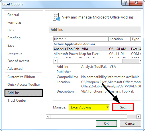
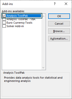
- Click on “FILE” and “Options”.

- Click on “Add-Ins.”

- Under “Add-Ins”, select “Excel Add-Ins” from the “Manage” options and click on “Ok.”

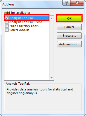
- Now, from the below window, select “Analysis Toolpak” and click on “OK” to enable “Data Analysis”.


You should see “Data Analysis” under the “DATA” tab.
How to do ANOVA Test in Excel?
Following is an example of how to do an ANOVA test in Excel.
You can download this ANOVA Excel Template here – ANOVA Excel Template
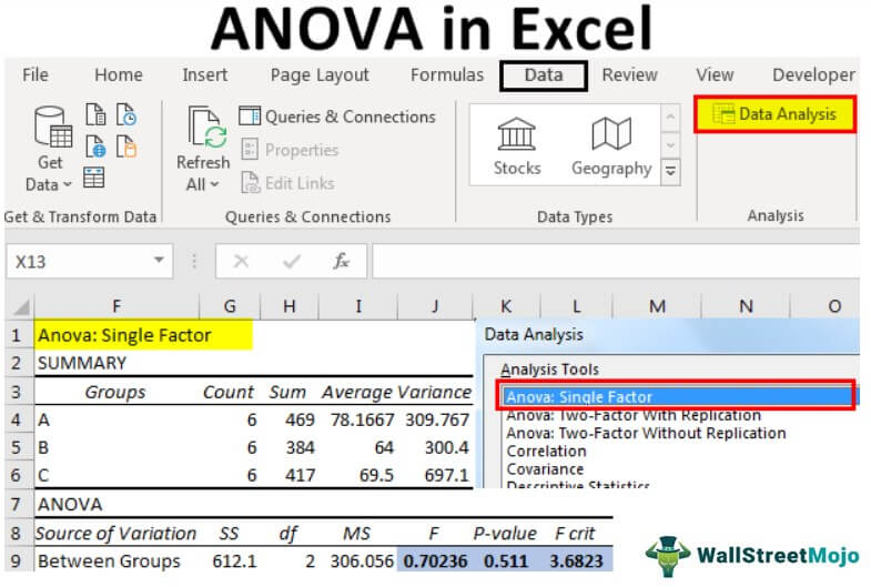
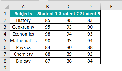
For this example, consider the below data set of three students’ marks in 6 subjects.
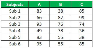
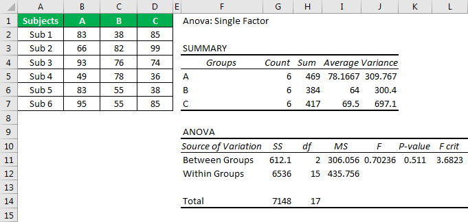
Above are students’ A, B, and C scores in 6 subjects. Now, we need to identify whether the scores of three students are significant or not.
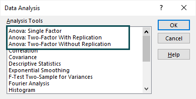
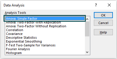
- Step 1: Click on “Data Analysis ” under the Data tab.”
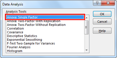
- Step 2: In the “Data Analysis” window, select the first option, “Anova: Single Factor.”
- Step 3: In the next window for “Input Range,” select student scores.
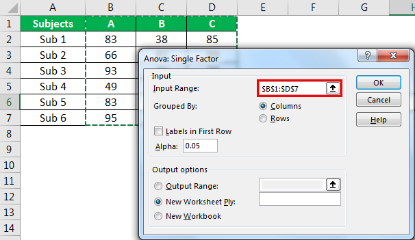
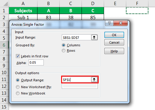
- Step 4: Since we have selected the data with headers, check the box “Labels in First Row.”

- Step 5: Now select the “Output Range” as one of the cells in the same worksheet.
- Step 6: Click on “OK” to complete the calculation. Now we will have a detailed “Anova: Single Factor” analysis.
Before we interpret the results of ANOVA, let us look at the hypothesis of ANOVA. Then, to compare the Excel ANOVA test results, we can frame two hypotheses – the “Null hypothesis” and “Alternative hypothesis.”
The null hypothesis is “there is no difference between scores of three students.”
The alternative hypothesis is that “at least one of the mean is different.”
If “F value > F critical value,” we can reject the null hypothesis.
If “F value < F critical value,” we cannot reject the null hypothesis.
If “p-value < alpha value,” we can reject the null hypothesis.
If “p-value > alpha value,” we cannot reject the null hypothesis.
Note: alpha value is the significance level.
You may not go back and look at the result of ANOVA.
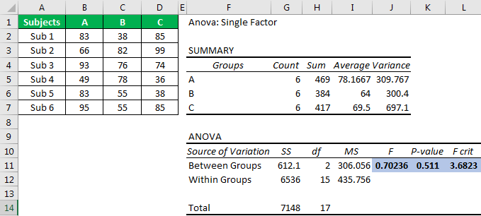
First, look at the “p-value,” which is 0.511. Unfortunately, it is greater than the alpha or significance value (0.05), so we cannot reject the null hypothesis.
Next, the F value of 0.70 is less than the F critical value of 3.68, so we cannot reject the null hypothesis.
Next, the F value of 0.70 is less than the F critical value of 3.68, so we cannot reject the null hypothesis.
Things to Remember
- You need strong ANOVA knowledge to understand things better.
- Always frame the null hypothesis and the alternative hypothesis.
- If the F value > F critical value,” then we can reject the null hypothesisNull hypothesis presumes that the sampled data and the population data have no difference or in simple words, it presumes that the claim made by the person on the data or population is the absolute truth and is always right. So, even if a sample is taken from the population, the result received from the study of the sample will come the same as the assumption.read more
- “If F value < F critical value,” we cannot reject the null hypothesis.
Recommended Articles
This article has been a guide to ANOVA in Excel. Here, we discuss how to do the ANOVA test in Excel with the help of an example and a downloadable Excel sheet. You can learn more about Excel from the following articles: –
- Work Breakdown Structure in Excel
- Use Logical Functions in Excel
- Descriptive Statistics Excel
- Exponential Smoothing in Excel
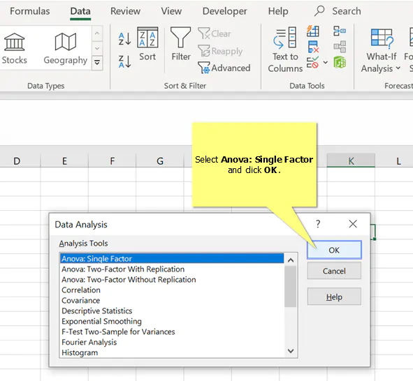
How to use one-way ANOVA in Excel
- Click the Data tab.
- Click Data Analysis.
- Select Anova: Single Factor and click OK.
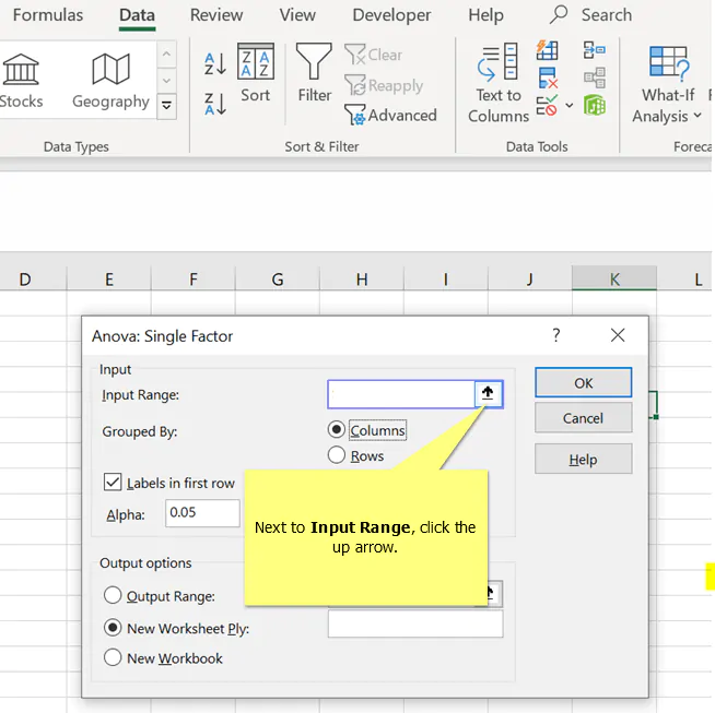
- Next to Input Range click the up arrow.
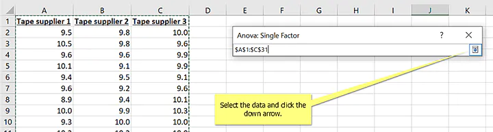
- Select the data and click the down arrow.
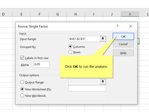
- Click OK to run the analysis.
Contents
- 1 What is Anova in Excel?
- 2 How do you use a Anova?
- 3 What is an example of ANOVA?
- 4 How do you do an ANOVA table?
- 5 Why do we use ANOVA?
- 6 What is two way Anova used for?
- 7 What is ANOVA used for in statistics?
- 8 What are the 3 types of ANOVA?
- 9 What is ANOVA in simple words?
- 10 What is p value in ANOVA?
- 11 How do you write ANOVA results?
- 12 What is the difference between one-way and two-way ANOVA?
- 13 When would you use a two-way ANOVA example?
- 14 Can ANOVA be used for 2 groups?
- 15 Can Anova be used for continuous data?
- 16 What variables are in an Anova?
- 17 What are the limitations of Anova?
- 18 What does P value of 0.05 mean?
- 19 What does F crit mean in ANOVA?
What is Anova in Excel?
ANOVA (Analysis of Variance) in Excel is the single and two-factor method used to perform the null hypothesis test, which says if the test will be PASSED for Null Hypothesis if all the population values are exactly equal to each other.
How do you use a Anova?
Steps
- Find the mean for each of the groups.
- Find the overall mean (the mean of the groups combined).
- Find the Within Group Variation; the total deviation of each member’s score from the Group Mean.
- Find the Between Group Variation: the deviation of each Group Mean from the Overall Mean.
What is an example of ANOVA?
ANOVA tells you if the dependent variable changes according to the level of the independent variable. For example: Your independent variable is social media use, and you assign groups to low, medium, and high levels of social media use to find out if there is a difference in hours of sleep per night.
How do you do an ANOVA table?
How to Perform a One-Way ANOVA by Hand
- Step 1: Calculate the group means and the overall mean. First, we will calculate the mean for all three groups along with the overall mean:
- Step 2: Calculate SSR.
- Step 3: Calculate SSE.
- Step 4: Calculate SST.
- Step 5: Fill in the ANOVA table.
- Step 6: Interpret the results.
Why do we use ANOVA?
You would use ANOVA to help you understand how your different groups respond, with a null hypothesis for the test that the means of the different groups are equal. If there is a statistically significant result, then it means that the two populations are unequal (or different).
What is two way Anova used for?
A two-way ANOVA test is a statistical test used to determine the effect of two nominal predictor variables on a continuous outcome variable. A two-way ANOVA tests the effect of two independent variables on a dependent variable.
What is ANOVA used for in statistics?
ANOVA stands for Analysis of Variance. It’s a statistical test that was developed by Ronald Fisher in 1918 and has been in use ever since. Put simply, ANOVA tells you if there are any statistical differences between the means of three or more independent groups. One-way ANOVA is the most basic form.
What are the 3 types of ANOVA?
A recap of 2-way ANOVA basics
Three different methodologies for splitting variation exist: Type I, Type II and Type III Sums of Squares. They do not give the same result in case of unbalanced data. Type I, Type II and Type III ANOVA have different outcomes!
What is ANOVA in simple words?
Analysis of variance, or ANOVA, is a statistical method that separates observed variance data into different components to use for additional tests. A one-way ANOVA is used for three or more groups of data, to gain information about the relationship between the dependent and independent variables.
What is p value in ANOVA?
The p-value is the area to the right of the F statistic, F0, obtained from ANOVA table. It is the probability of observing a result (Fcritical) as big as the one which is obtained in the experiment (F0), assuming the null hypothesis is true.
How do you write ANOVA results?
When reporting the results of a one-way ANOVA, we always use the following general structure:
- A brief description of the independent and dependent variable.
- The overall F-value of the ANOVA and the corresponding p-value.
- The results of the post-hoc comparisons (if the p-value was statistically significant).
What is the difference between one-way and two-way ANOVA?
A one-way ANOVA only involves one factor or independent variable, whereas there are two independent variables in a two-way ANOVA. 3. In a one-way ANOVA, the one factor or independent variable analyzed has three or more categorical groups. A two-way ANOVA instead compares multiple groups of two factors.
When would you use a two-way ANOVA example?
You should use a two-way ANOVA when you‘d like to know how two factors affect a response variable and whether or not there is an interaction effect between the two factors on the response variable. For example, suppose a botanist wants to explore how sunlight exposure and watering frequency affect plant growth.
Can ANOVA be used for 2 groups?
Typically, a one-way ANOVA is used when you have three or more categorical, independent groups, but it can be used for just two groups (but an independent-samples t-test is more commonly used for two groups).
Can Anova be used for continuous data?
An analysis of variance (ANOVA) is an appropriate statistical analysis when assessing for differences between groups on a continuous measurement (Tabachnick & Fidell, 2013).This type of analysis is applied when examining for differences between independent groups on a continuous level variable.
What variables are in an Anova?
THE VARIABLES IN THE ONE-WAY ANOVA In an ANOVA, there are two kinds of variables: independent and dependent. The independent variable is controlled or manipulated by the researcher. It is a categorical (discrete) variable used to form the groupings of observations.
What are the limitations of Anova?
What are some limitations to consider? One-way ANOVA can only be used when investigating a single factor and a single dependent variable. When comparing the means of three or more groups, it can tell us if at least one pair of means is significantly different, but it can’t tell us which pair.
What does P value of 0.05 mean?
A statistically significant test result (P ≤ 0.05) means that the test hypothesis is false or should be rejected. A P value greater than 0.05 means that no effect was observed.
What does F crit mean in ANOVA?
Your F crit or alpha value is the risk that you are willing to be wrong in rejecting the null. The higher the F value, the smaller the remaining area to the right and thus the p value.
An important part of being ready for a successful six sigma project is being familiar with the analyses that you’ll use to measure improvement in your processes.
One of the more useful analyses in your toolbelt can be the Analysis of Variance, commonly abbreviated ANOVA.
ANOVA covers a range of common analyses. Some analyses have names related to the number of factors, such as one-way ANOVA and two-way ANOVA. When the levels of a factor are selected at random from a wide number of possibilities, you might use a random-effects model or a mixed-effects model.
And luckily, Microsoft Excel makes it easy to perform these analyses. So we’re going to go through how to use ANOVA in Excel.
Download your data files
Follow along with the steps in the article by downloading these practice files
What is ANOVA?
While ANOVA has many varieties, the essential purpose of this family of analyses is to determine whether factors have an association with an outcome variable.
Factors are the variables that you will use to categorize your outcome variable into groups. For example, if you want to know whether tapes from three different suppliers have the same peel strength, the suppliers are your factor. All the strength measurements for the same supplier’s tape form a group of measurements.
ANOVA is an inferential statistical analysis.
Inferential analysis is the formal way of saying that we want to look at a sample of measurements and make an educated guess about what all of the possible measurements might be like if we could take them.
Let’s return to the tape example. If you could tape 1 million boxes from a batch of tape, those million might represent the entire population that we want to know about. But if we taped those million boxes and measured the peel strength, we would have used up all of the tape. Instead, we’ll measure the strength from a sample of taped boxes and use those measurements to guess what the numbers would look like if we taped a million boxes.

What does ANOVA do?
An important point is that we won’t expect all the measurements in a group to be the same.
Consider the tape example again. The differences in strength measurements from the same supplier’s tape give us within-group variation. Another important point is that we won’t expect the average strength of our sample to be the same as the average strength if we taped a million boxes. This variation between the sample average and the overall average we’ll call bias.
Because of within-group variation and bias, comparisons among groups become harder. We’ll know that our sample average is not the same as the real average, there’s no easy way to know when our guess is too high or too low. If we guess too high for one group and too low for another group, we might easily reach an incorrect conclusion, such as predicting that the supplier with the strongest tape on average has the weakest tape.
ANOVA gives us mathematical sets of rules, that hold certain given assumptions, to decide when we can have confidence that the real average of one group is different from the real average of one or more other groups. ANOVA sets up these rules by asking how sure we are that the means are the same, a concept that we refer to as the null hypothesis. Remember that the null hypothesis is a useful concept for helping us make comparisons, even though we already know that for real group averages to all be the same would be a remarkable coincidence.
Most of the time, a key result of an ANOVA analysis is a p-value. The p-value has meaning only with respect to the null hypothesis of the ANOVA analysis. For one-way ANOVA, the null hypothesis is that the means for each level of your factor are the same.
A rough interpretation would be that the p-value reflects how much confidence you can have that the null hypothesis is a reasonable model. Small p-values make you think that the null hypothesis is not a reasonable model. Large p-values might lead you to act like the null hypothesis is true, even though you know that it’s not really true, just a reasonable model.
To learn more check out this glossary of Lean Six Sigma terms
Let’s work through a practical example in Excel. We’ll begin with one-way ANOVA, which looks at the effect of a single factor.
The Data Analysis Toolpak in Excel
If you’re analyzing data in Excel, then it’s natural to make use of the tools that Microsoft provides for you. One of the less obvious features in Excel is the Data Analysis Toolpak. The Toolpak is an Excel add-in from Microsoft that’s included with Excel, but isn’t turned on.
Here’s how to turn it on in the Microsoft Windows operating system.
- Choose File, then Options
- In the Excel Options Window, choose Add-ins
- Next to Manage, select Excel Add-ins and click Go
- In the Add-ins window, select Analysis ToolPak and click OK
 A new button on your Data ribbon will appear.

Example of one-way ANOVA in Excel’s Data Analysis Toolpak
While it can sometimes seem like a simple analysis will have the fewest applications, it’s easy to find practical ways to use one-way ANOVA. Essentially, you can use it anytime you have only one set of groups to compare.
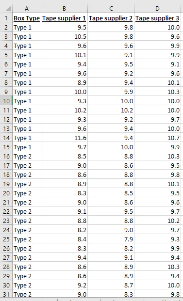
Let’s keep going with our tape example. You’ve invested in an automatic taping machine that applies heat to tape to create strong bonds. You’ve decided that you’re going to measure the strengths of tape samples from different suppliers yourself so that you can see whether there’s any practical difference in the strengths of the bonds using your machine and your boxes.
Data arrangement for one-way ANOVA in Excel
If you’ve been using Excel for a long time, you’ve gotten used to the idea that the spreadsheet is cell-based. That is, there’s very little difference between putting numbers in the spreadsheet in rows or in columns.
Data in rows:
Data in columns:
Microsoft’s been nice enough to make it so that their one-way ANOVA feature can work either way, but I’ll recommend that you start putting your data in columns. The data arrangement will matter when you want to use some of the other offerings in the Data Analysis Toolpak or a software package for data analysis, like Minitab Statistical Software.
If you’d like to follow along with data that’s already prearranged, you can use the following Excel file:
Download your data files
Follow along with the steps in the article by downloading these practice files
How to use one-way ANOVA in Excel
With the Data Analysis Toolpak installed and your data in columns, you can perform the following steps in Excel to get the results of the one-way ANOVA analysis.
1. Click the Data tab

2. Click Data Analysis
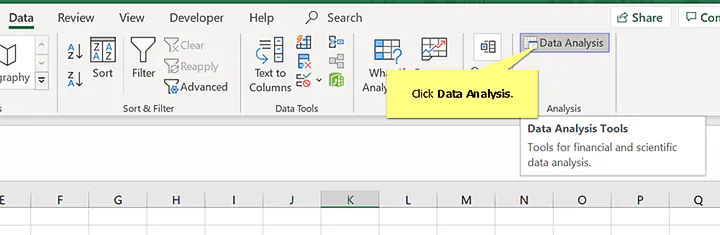
3. Select Anova: Single Factor and click OK
4. Next to Input Range click the up arrow
5. Select the data and click the down arrow
6. Click OK to run the analysis
Results for one-way ANOVA in Excel: Summary statistics
The results will look like this
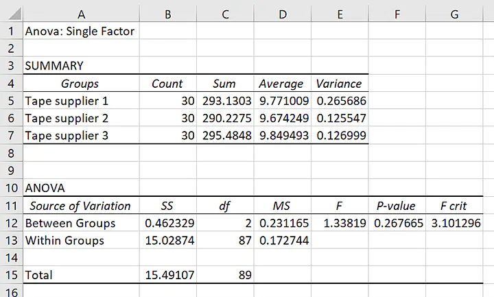
First, let’s take a minute to look at the summary statistics of each group.
In particular, the averages, in ascending order, are about 9.67, 9.77, and 9.84. That is, each of the tapes holds almost 10 kg before breaking. The difference between the largest mean and the smallest mean is about 0.17 kg. If kilograms aren’t very familiar to you, you can think of the tape with the lowest average being strong enough to hold about 60 apples and the tape with the highest average being strong enough to hold about 62 apples.
That should be enough for us to start to think about what we expect about the null hypothesis for the ANOVA. If you think that the means are similar, then you’ll expect to see a larger p-value for the hypothesis test.
Results for one-way ANOVA in Excel: Hypothesis tests
Remember that small p-values give us low confidence in the null hypothesis.
The value of about 0.27 is higher than the level where people traditionally agree that there is strong evidence against the null hypothesis. While most people learn 0.05 as a traditional cutoff, that value is mutable depending on the consequences of making an error either by deciding to act as if the means are the same or by acting like the means are not all the same.
Even so, 0.27 is such a large p-value that a lot of uncertainty remains about whether any of the averages are different. By extension, there’s a lot of uncertainty about whether any one average is larger than another.
 If those 2 apples worth of strength are so much that you would make a different decision about the tape suppliers because of that difference, then you’ll need more data.
On the other hand, if those 2 apples don’t sound like a big deal, this is a good place to decide that you can choose the supplier with other criteria. For example, you might consider price or your confidence that the supplier can fill your orders on time.
What if you have more factors?
Let’s suppose that you’re considering not only the tape supplier, but also choosing among some different boxes.
You know that the roughness and absorbency of the box might affect how strong the tape holds to it. Instead of doing the test only on the factor of tape supplier, you want to make sure that you have the right tape for the right box.
One approach could be to do a one-way ANOVA where you use more than one factor to define the groups. For example, one of the groups might be the first tape supplier on the first box type. Another group might be the second tape supplier on a second box type.
The disadvantage of this approach is that it doesn’t let you distinguish the effect of different factors. If the one-way ANOVA said that there was a difference between those two groups, then you still wouldn’t know how much of the difference was from the change in tape, the change in box, or a change that depended on both simultaneously.
An analysis to get this type of information when you have two factors is two-way ANOVA.
Data Arrangement for Two-Way ANOVA in Excel
Excel can be flexible with your data arrangement for one-way ANOVA, but is strict about the data arrangement when you do a two-way ANOVA with replication through the Data Analysis Toolpak. Data for one factor need to be in different columns.
Data for the second factor need to be in consecutive rows.
For Excel to work, you’ll need to have the same number of measurements for all of your groups.
You don’t necessarily have to provide the factor label for the rows, but it’s good practice, especially if you might want to graph your data in Excel later. This data arrangement, called a two-way table, would look like this:
 If you’d like to follow along with data that’s already prearranged, you can use the following
Download your data files
Follow along with the steps in the article by downloading these practice files
How to use two-way ANOVA in Excel
With the Data Analysis Toolpak installed and your data in columns, you can perform the following steps in Excel to get the results of the two-way ANOVA analysis. You’ll begin as you did for one-way ANOVA.
Follow along with the two-way ANOVA steps
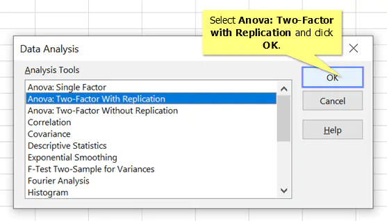
1. Click the Data tab

2. Click Data Analysis
3. Select Anova: Two Factor with Replication and click OK
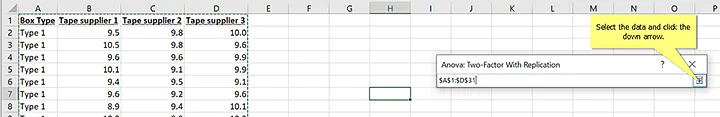
4. Next to Input Range, click the up arrow
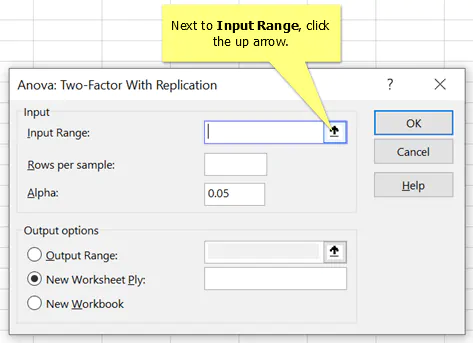
5. Select the data and click the down arrow
6. In Rows per sample, enter the number of measurements in the group, then click OK to run
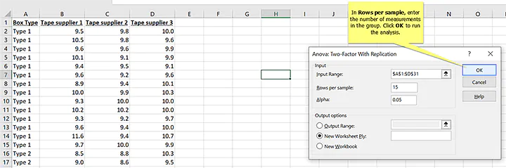 In this data, you can see that rows 2 to 15 have the measurements for the first box type. Those rows have 15 data points. Since the groups all have to have the same amount of data for the analysis to work in Excel, we know that the second box type must also have 15 rows.
Results for two-way ANOVA in Excel: Summary statistics
As with one-way ANOVA, your results will come in two parts. The first part will be summary statistics about your groups. I’ve added the highlighting.
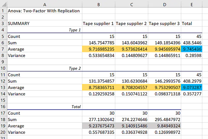
The blue highlighting shows the overall averages for the two different box types in the data. The difference is about 0.67 kilograms. The gray highlighting shows the averages for the 3 different tape suppliers. The averages for tape supplier 3 is closest to 10, while the averages for tape suppliers 1 and 2 are closer to 9.
The averages for the individual groups have gold highlighting. If the tapes from the different suppliers all work the same on both types of boxes, then the averages for the individual groups should follow the same patterns: The average for box type 1 should be higher and the average for tape supplier 3 should be higher.
The group averages show a different pattern than the overall averages for the two factors. Tape supplier 3’s average is higher than the other two because there is a larger difference between the suppliers for the second box type.
This comparison of the averages should prepare us for what to expect about the null hypothesis for two-way ANOVA that the factors do not affect the response variable.
Results for two-way ANOVA in Excel: Hypothesis tests
For our one-way ANOVA analysis, the p-value was relatively large. That value led us to conclude that we couldn’t be certain whether there was any difference between the tape suppliers.
For the two-way ANOVA, our largest p-value is about 0.002. That is much smaller than the traditional cutoff value for statistical significance of 0.05.
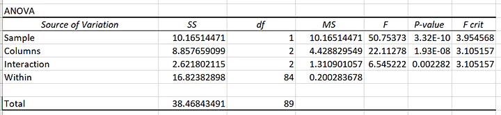
Because the p-value for the interaction is small, we cannot make a simple statement that one supplier or box type leads to a higher peel strength.
The hypothesis test confirms what we might have expected from the examination of the averages: The effect of the different tapes depends on the box type. (We could equivalently say that the effect of the different box types depends on the tape.)
From the default results in Excel, you can conclude that not all of the groups have the same peel strength. To make a more precise statement about the relationships among the groups, you should proceed to a multiple comparisons analysis.
Bonus tutorial: Selecting which hypothesis test to use
If you want to learn about the various types of hypothesis tests, then check out this video tutorial on hypothesis testing:
Conclusion
While the examination of the averages for the two-way ANOVA analysis suggests that the choice of tape matters only if you’re going to use the second box type, you’ll want to consider your decisions carefully from both a statistical and a practical perspective.
If you need the tape to have a peel strength of only 5 kilograms, then the peel strengths are probably all adequate. If a difference of 0.4 kilograms might lead you to choose one group over another, then more analysis of the data is in order.
You can learn more techniques for analyzing ANOVA data in this course on hypothesis testing. If you’ve already acquired the basics, then you’re ready to proceed to more advanced considerations in this design of experiments course. Either way, the knowledge that you gain will help you prepare to ensure that your projects exceed your expectations.
Prepare to get certified in Lean Six Sigma
Start learning today with GoSkills courses
Start free trial
What Is ANOVA In Excel?
ANOVA or Analysis of Variance, is a statistical analysis that evaluates whether the mean values of two or more independent groups are significantly different or not. ANOVA In Excel assesses the impact of one or multiple factors by comparing different mean values. It helps users understand the variance of variables, and they can use it to perform null hypothesis testing and regression analysis.
For example, the following table contains the score details of three students.
Using the single-factor ANOVA in Excel technique, we can examine if the mean values of the three datasets i.e., the scores of Students 1, 2, and 3, are the same or significantly different.
Now, we can see whether to accept or reject the null hypothesis if there is no significant difference in the mean values of Student 1, Student 2, and Student 3 scores.
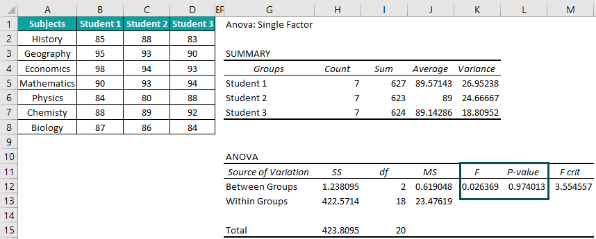
Once we calculate ANOVA in Excel, we get the output shown in the above image.
Output Observation: The F and p-value are the most critical parameters in an ANOVA in Excel. In the above example, the F value is less than the F crit value (F critical). Also, the p-value is more than Alpha, the significance threshold (typically 0.05). Thus, we cannot reject the null hypothesis, and the mean values of the three students’ scores are not significantly different.
Table of contents
- What Is ANOVA In Excel?
- Where Is ANOVA In Excel?
- One Way ANOVA Test In Excel
- Two Way ANOVA Test In Excel
- #ANOVA: Two-Factor with Replication
- #ANOVA: Two-Factor Without Replication
- ANOVA In Excel Interpretation
- Important Things To Note
- Frequently Asked Questions
- Download Template
- Recommended Articles
- ANOVA in Excel is a statistical method used to determine if the mean values of various groups in a model are significantly different or not.
- Excel offers three types of ANOVA tests, single-factor, two-factor with replication, and two-factor without replication.
- The Analysis Tools list in the Data Analysis window will show the ANOVA tests.
- The F and p-value are the two most important parameters we need to check in the ANOVA test result. They decide whether to accept or eliminate the null hypothesis and determine which independent variables affect the dependent variable.
Where Is ANOVA In Excel?
Although the function exists, ANOVA in Excel is not enabled by default.
Initially, the “Data” tab will be as shown below.

Let us first enable the Excel add-in “Analysis ToolPak” so that we can calculate ANOVA in Excel.
The steps to enable the Analysis ToolPak add-in are:
Step 1: Choose File > Options to open the Excel Options window.


Step 2: Click the Add-ins option on the left in the Excel Options window. On the right side, below, check if the Manage field is Excel Add-ins, and click Go… to open the Add-ins window.

Step 3: In the Add-ins window, check/tick the “Analysis ToolPak” checkbox and click “OK”.
Once we click “OK”, the “Data” tab will show the “Data Analysis” option.

Now, select the “Data” tab > go to the “Analysis” group > click the “Data Analysis” option to open the “Data Analysis” window to access the ANOVA functions.
In the “Data Analysis” window, we see the ANOVA options in the “Analysis Tools” list.
The first option will enable us to perform a one-way ANOVA test or single-factor ANOVA in Excel. We can conduct a two-way ANOVA test in Excel with the other two options.
One Way ANOVA Test In Excel
The one-way ANOVA test compares the mean values of datasets and determines if they are different. We will use the “ANOVA: Single Factor” option from the “Data Analysis” window.
The following table shows the tensile strength data collected during three tests.

The steps to conducting the One-Way ANOVA Test in Excel are:
1: Select the “Data” tab > go to the “Analysis” group > click the “Data Analysis” option.
2: Once the Data Analysis window opens, choose the first option i.e., “ANOVA: Single Factor”, from the “Analysis Tools” list.
3: Click “OK” > the “ANOVA: Single Factor” window opens. Add the details as shown below.
- Go to the “Input” group > enter the data range in the “Input Range” field as A1:C9, choose “Grouped By:” as “Columns”, and check/tick the “Labels in first row” [Note: The Alpha value will be 0.05 by default].
- Now, go to the “Output Options” group > select the “Output Range:” option > enter the cell as F1 in the “Output Range:” field.

[Note:
- To display the output in the current sheet, select the “Output Range:” option in the “Output Options” group and enter the target cell to show the ANOVA in Excel test result.
- To display the output in a new spreadsheet, select the “New Worksheet Ply:” option in the “Output Options” group, and enter the target cell.]
4: Click “OK” in the “ANOVA: Single Factor” window. We will get the following output.

Output interpretation: We will now understand the ANOVA in Excel meaning of the above result.
The F value is 0.00121. It is less than the F crit value, 3.4668. And the p-value is 0.998, which is more than the Alpha value, 0.05. Thus, we cannot eliminate the null hypothesis that the mean values of the three datasets representing the three tests are not significantly different.
Two Way ANOVA Test In Excel
A two-way ANOVA test in Excel helps determine the effect of two independent variables on a dependent variable. We will use the following options from the “Data Analysis” window.
- ANOVA: Two-Factor with Replication.
- ANOVA: Two-Factor Without Replication.
#ANOVA: Two-Factor with Replication
The following table shows five men’s balanced diet intake, exercise frequency, and weight loss data.

The steps to find the Two-Way ANOVA Test using the ANOVA: Two-Factor with Replication are:
1: Select the “Data” tab > go to the “Analysis” group > click the “Data Analysis” option.
2: Once the Data Analysis window opens, choose the first option i.e., “ANOVA: Two-Factor With Replication”, from the “Analysis Tools” list.

3: Click “OK” > the “ANOVA: Two-Factor With Replication” window opens. Add the details as shown below.
- Go to the “Input” group > enter the data range in the “Input Range” field as A2:D12 > enter 5 in the “Rows per sample:” field, as there are five men. [Note: The Alpha value will be 05 by default].
- Now, go to the “Output Options” group > select the “Output Range:” option > enter the cell as G1 in the “Output Range:” field.
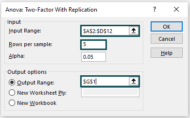
4: To get the output in the current sheet, set the “Output Range” as the target cell in the current sheet. Finally, click “OK” in the “ANOVA: Two-Factor With Replication” window. We will get the following output.

Output interpretation: We will now understand the ANOVA in Excel meaning of the above result.
Consider the last table, ANOVA. The Sample field refers to Exercise Frequency, and the Columns field indicates Balanced Diet Intake. Now observe the p-value.
- The p-value of Exercise Frequency is 68E-05. It is statistically significant as it is less than the Alpha value of 0.05.
- The p-value of Balanced Diet Intake is 01E-07. It is statistically significant as it is less than the Alpha value of 0.05.
- The p-value for the interaction between Exercise Frequency and Balanced Diet Intake is 228173. So, it is not statistically significant as it is greater than the Alpha value of 0.05.
Thus, these observations indicate that both factors, Exercise Frequency and Balanced Diet Intake, have a statistically significant impact on weight loss. And they are the main effects in this example model.
Also, the significant p-values prove that the mean values for the five men sample data are not equal. The Average field in the SUMMARY table corroborates the above observation.
On the other hand, there is no interaction effect. So, whether a person exercises daily or weekly, it does not affect how they lose weight due to a balanced diet. Instead, the main effects are the section of the relationship between the independent and the dependent variables that do not get modified based on the other variables’ values.
#ANOVA: Two-Factor Without Replication
The two-factor ANOVA in Excel without replication is an extension of the single-factor ANOVA test, except there are two independent variables instead of one factor. Therefore, we can follow the above-explained steps to determine it. But the ANOVA test type in the Data Analysis window is “ANOVA: Two-Factor Without Replication”.
But, while the ANOVA test without replication helps analyze the effects of the independent variables on the dependent variable, we cannot review the interaction between them.
ANOVA In Excel Interpretation
The ANOVA in Excel results or output consists of two tables, SUMMARY and ANOVA.
The SUMMARY table shows the sample Count, Sum, Average, and Variance data for each group in the model.
- Count: It is the number of samples in each group in the model.
- Sum: It is the sum of values in each group in the model.
- Average: The result obtained from dividing the Sum by Count for each group in the model.
- Variance: The data points’ dispersion level from the respective group mean value.
The ANOVA table shows the values SS, df, MS, F, P-value, and F crit for each source of variation.
- SS: It is the sum of squares for each source of variation.
- df: It denotes the degree of freedom associated with each variance source.
- MS: It shows the mean square.
- F: It shows the F-statistic used during the null hypothesis test to determine the model’s significance. It is the result of dividing variation between the sample means and variation within the samples.
- P-value: The probability determines the evidence against the null hypothesis.
- F crit: The parameter stands for F critical. It is the F-statistic value at the threshold probability, Alpha, of wrongly eliminating a null hypothesis.
When we perform a test for ANOVA in Excel, we need to check the F and p-value in the result to interpret the output and determine the model’s significance.
We cannot eliminate the null hypothesis in a single-factor ANOVA test if the F value is less than the F crit value. Likewise, we cannot reject the null hypothesis if the p-value is higher than the Alpha value.
In a two-way ANOVA test with replication, the factor or independent variable with a significant p-value (i.e., a p-value less than the Alpha value) affects the dependent variable. And a significant p-value of Interaction indicates the relationship between an independent and the dependent variables gets modified based on the other independent variable value.
On the other hand, the ANOVA test interpretation remains the same for a two-way ANOVA test without replication, except there will be no interaction data to analyze.
Important Things To Note
- ANOVA in Excel helps perform analysis of variance and tests such as null hypothesis testing for models involving three or more independent groups.
- Enable the Analysis ToolPak add-in to get the Data Analysis feature added to the Data tab required to perform the ANOVA tests.
- If the F value is less than the F crit value or the p-value is more than the Alpha value in a one-way ANOVA test, we cannot eliminate the null hypothesis.
- The factor or independent variable with a significant p-value (i.e., a p-value less than the Alpha value) affects the dependent variable in a two-way ANOVA test.
Frequently Asked Questions
What is ANOVA in Excel used for?
ANOVA in Excel is used to check whether the mean values of various groups in a dataset are significantly different. It evaluates the effect of one or more independent variables or factors on a dependent variable by comparing the mean values of different samples.
Which ANOVA in Excel to use?
We can use the one-factor or two-factor ANOVA in Excel. And we have two options available for the two-factor or two-way ANOVA test, one with replication and the other without replication.
How to run an ANOVA in Excel?
We can run an ANOVA in Excel using the below steps:
Step 1: In the current worksheet, choose Data > Data Analysis to open the Data Analysis window.
Step 2: Select the ANOVA test we require to perform for our model from the Data Analysis window.
Once we choose the required ANOVA test from the three options highlighted in the above image and click OK, their respective dialog boxes pop up. Next, we will need to enter the input data and the location where we want to display the ANOVA test result i.e., whether in the current worksheet itself or a new worksheet and click OK to view the result.
What is F in ANOVA in Excel?
F in ANOVA in Excel is the parameter that determines the model significance in a null hypothesis.
Download Template
This article must help understand ANOVA in Excel, with its formula and examples. We can download the template here to use it instantly.
Recommended Articles
This has been a guide to ANOVA in Excel. Here we learn how to do One & Two Way ANOVA with/without replication, interpretations, examples & downloadable excel template. You can learn more from the following articles –
- Regression Analysis In Excel
- Descriptive Statistics in Excel
- Add-ins In Excel
Пусть имеется случайная переменная
Y
, значения которой мы можем измерять. Исследователь предполагает, что эта переменная зависит от фактора, значения которого мы можем контролировать, т.е. задавать с требуемой точностью. Покажем как методом дисперсионного анализа (
ANOVA
) проверить гипотезу о наличии или отсутствии влияния указанного фактора на зависимую переменную
Y
.
Disclaimer
: Эта статья – о применении MS EXCEL для целей
Дисперсионного анализа, поэтому
данную статью не стоит рассматривать, как пересказ главы из учебника по статистике. Статья не обладает ни полнотой, ни строгостью изложения положений статистической науки. Теоретические отступления приведены лишь из соображения логики изложения. Использование данной статьи для изучения теории
Дисперсионного анализа
– плохая идея. Хорошая идея — найти в этой статье формулы MS EXCEL для проведения
Дисперсионного анализа.
Перед прочтением этой статьи рекомендуется освежить в памяти следующие понятия статистики:
-
Проверка статистических гипотез
;
-
Дисперсия
и
среднее значение
;
-
Распределение Фишера
и
квантили
этот распределения;
-
F-тест
;
-
Блочные диаграммы
.
Дисперсионный анализ
(ANOVA, ANalysis Of VAriance) позволяет
проверить гипотезу
о равенстве нескольких
средних значений
выборок (взяты ли выборки из одного распределения или из разных распределений).
Примечание
: В статье
Двухвыборочный t-тест с одинаковыми дисперсиями
решалась подобная задача о сравнении
средних значений
2-х распределений. Здесь рассмотрим более общую задачу – будем одновременно сравнивать несколько
средних значений
выборок (более 2-х).
Чтобы пояснить суть
дисперсионного анализа
приведем пример.
Сгенерируем
2 выборки: первую возьмем из
нормального распределения
со средним значением равно 4, вторую со средним — 5 (
стандартные отклонения
одинаковые). Сказать, сильно ли они различаются или нет, невозможно, пока мы не знаем разброс (стандартное отклонение) значений в каждой выборке относительно среднего. Если зададим в распределениях небольшой разброс, скажем 0,1, то в каждой выборке получим близкое к нему значение. В этом случае, очевидно, что наблюдаемое различие между
средними
равное 1 (5-4=1) – значительное и можно говорить, что выборки взяты из разных распределений (см. картинку ниже).

Если же разброс в выборках составляет около 2, то наблюжаемое различие средних значений выборок равное 1 уже не кажется таким значительным.
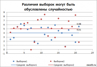
В дисперсионном анализе эти значения выборок представляют собой значения зависимой переменной Y, а выборки берутся при различных уровнях фактора Х. В первом случае для того дать ответ о зависимости Y от фактора Х, даже не нужно проводить
дисперсионный анализ
: из диаграммы итак очевидно, что отличие между средними значениями выборок (5-4=1), гораздо больше разброса внутри выборки (0,1). Следовательно, очевидно, что выборки взяты из различных генеральных совокупностей (с различными распределениями), которые соответствуют разным значениям Х.
Во втором случае без
дисперсионного анализа
не обойтись. Различие между
средними значениями
может быть обусловлено просто случайностью выборок, взятых из одного распределения.
В конце статьи мы определим математически точно условие «значимости» различия
средних выборок
.
Немного теории
Примечание
: Пользователи, уверенно владеющие методом
дисперсионного анализа
, могут перейти непосредственно к
формулам MS EXCEL
.
Пусть необходимо исследовать зависимость некой
количественной
случайной величины Y от одной переменной, которую мы можем контролировать (устанавливать их значения с требуемой точностью). В теории
дисперсионного анализа
переменная Y называется
зависимой переменной
(
dependent
или
response
variable
), а переменные, от которых исследуется зависимость переменной Y, называются факторами или зависимыми переменными (
factors
или
dependent
variables
).
Для целей этой статьи будем предполагать, что Y зависит только от одного фактора.
Примечание
: Случай зависимости от 2-х факторов рассмотрен в статье
Двухфакторный дисперсионный анализ
.
Отдельные, заданные значения фактора называются уровнями (
levels
) или испытаниями (
treatments
).
Так как мы можем контролировать значения, которые принимает
фактор
, то данные (набор значений Y), которые получены в результате испытаний, мы назовем
экспериментальными
, а сам процесс получения этих данных —
экспериментом
.
Целью эксперимента является исследование влияния различных уровней фактора на переменную Y. В самом деле, так как фактор нами контролируется, то у нас есть возможность сделать несколько наблюдений (измерений) величины Y при определенном заданном уровне фактора. Зачем их делать несколько, ведь значения Y должны получиться одинаковыми? Нет. Так как мы предполагаем, что на переменную Y может влиять множество неконтролируемых нами факторов, то мы будем получать в ходе каждого измерения несколько отличающиеся значения Y. Единственное, что мы можем сделать, это обеспечить одинаковые условия проведения эксперимента для всех измерений.
Например, измеряя расход бензина на 100 км/ч одной и той же марки бензина на одном и том же автомобиле, мы будем получать несколько различные значения. Может непредсказуемо измениться направление ветра, состояние дороги или автомобиля, что в свою очередь повлияет на расход.
Уровни фактора (treatments) будем обозначать буквой j (j изменяется от 1 до
a
). Каждому уровню фактора соответствует одна выборка (состоит из нескольких измерений). Предполагается, что
дисперсии
всех выборок σ
2
неизвестны, но равны между собой.
Непосредственно измеренные значения Y при заданном уровне фактора j будем обозначать y
ij
. Количество наблюдений для разных уровней факторов может быть одинаковым или отличаться.
Примечание
: Чем больше количество измерений/наблюдений (т.е. размер выборки) мы сделаем, тем более обоснованным будет наш статистический вывод о равенстве
средних значений
этих выборок.
В тексте статьи будем рассматривать только равные выборки, их размер обозначим n. В Этом случае общее количество измерений N=n*a.
Примечание
: В
файле примера
выполнены вычисления для обоих случаев (равные и неравные по размеру выборки).
Если фактор действительно оказывает влияние на зависимую переменную Y, то при различных уровнях фактора мы должны в среднем получать различные значения Y. Другими словами, мы должны получить «заметно различающиеся»
средние выборок
при различных уровнях фактора:
Остается выяснить, что значит средние выборок «заметно отличаются».
Стандартные обозначения дисперсионного анализа
Общий подход при проведении Дисперсионного анализа: проверить значимость различия средних значений выборок, сравнив один источник разброса (проверяемый фактор) с другим источником разброса (обоснованный лишь случайностью выборок/ случайным воздействием неконтролируемых факторов):
![]()
Введя нижеуказанные обозначения, выражение можно записать в компактной форме:
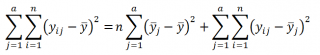
SST=SSA+SSE
Эти общеупотребительные обозначения расшифровываются следующим образом: SS – это сокращение английского выражения Sum of Squares (сумма квадратов отклонений от среднего), T – это сокращение от Total (Общее среднее), А – это фактор А, E – это сокращение от Error (ошибка).
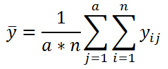
На основании данных определений, вышеуказанное выражение может быть преобразовано в вычислительную форму:
где,
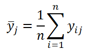
![]()
– общее среднее:
Обратите внимание, что квадраты отклонений имеют размерность
дисперсии
, т.е. меры изменчивости. Теперь очевидно, что левая часть выражения представляет собой общую изменчивость (разброс) каждого из наблюдений относительно общего среднего. Эта общая изменчивость (SST) состоит из двух частей: SSA — изменчивость, объясненная нашей моделью (междувыборочная изменчивость, основанная на различиях в уровнях фактора) и из SSE — ошибка модели (внутривыборочная изменчивость, сумма разбросов наблюдений внутри каждой выборки).
Также в
дисперсионном анализе
используется понятие
среднего квадрата отклонений
(Mean Square), т.е. MS. Соответственно для SST имеем MST=SST/(N-1), для SSA имеем MSA=SSA/(n-1), для ошибки модели SSE имеем MSE=SSE/(a(n-1)).
MS имеет смысл средней изменчивости на 1 наблюдение (с некоторой поправкой). Эта поправка отражает тот факт, что MS должна вычисляться не делением SS на соответствующее количество наблюдений, а на число
степеней свободы
(degrees of freedom, DF). Например, чтобы вычислить MST, мы из N (общего количества наблюдений) должны вычесть 1, т.к. в выражении SST присутствует одно
среднее значение
(аналогично тому, как мы делали при вычислении
дисперсии выборки
). Одна степень свободы теряется при вычислении среднего – это видно в формуле выражения для SST.
В SSA мы имеем уже
а
средних значений (равно количеству уровней фактора, т.е. количеству выборок). Поэтому, из общего количества наблюдений
a
*n необходимо вычесть
а
– количество вычисленных средний значений выборок (an-a=a(n-1)).
Напомним, что в
дисперсионном анализе
проверяется гипотеза о равенстве
средних значений
этих выборок. Т.е. формулируется нулевая гипотеза Н
0
, которая утверждает, что Y не зависит от фактора и все выборки, измеренные при различных уровнях фактора, на самом деле взяты из одного распределения с общим средним.
Идем дальше. Оказывается,
если нулевая справедлива
, то:
-
случайная величина MSА представляет собой оценку σ
2
-
отношение MSА/MSE имеет
распределение Фишера
с
а-1
и
a
(
n
-1)
степенями свободы.
MSА/MSE обозначают как F
0
(
тестовая статистика
для
однофакторного дисперсионного анализа
).
Примечание
: Можно показать, что MSE также представляет собой оценку σ
2
дисперсии выборок (
математическое ожидание
случайной величины MSE равно σ
2
). Но, в отличие от MSА, MSE представляет собой оценку σ
2
вне зависимости от того, справедлива ли нулевая справедлива или нет.
Теперь, введя основные понятия, рассмотрим вычислительную часть
дисперсионного анализа
на примере решения задачи.
Задача
В качестве задачи рассмотрим технологический процесс изготовления нити в химическом реакторе.
Пусть предполагается, что инженер исследует влияние некой добавки на
прочность нити
Y. Он решает провести эксперимент:
-
Использовать 4 различных концентраций добавки (1%; 5%; 7% и 10%).
Прим
.:
эти значения концентраций не участвуют в расчетах.
- Провести по 6 (n) измерений прочности нити для каждой концентрации добавки.
Таким образом, имеется только 1 фактор (концентрация добавки). Фактор имеет 4 (а=4) различные уровня (j=1; 2; 3; 4). Всего у нас имеется 24 (N=4*6) измерения.
Вроде бы эксперимент полностью описан, теперь инженеру требуется только провести измерения. Однако, есть еще одна сложность: на разброс результатов при различных уровнях фактора может повлиять то,
как
мы проводим эксперимент.
О рандомизированном эксперименте
Представим, что у нас есть только 1 реактор. Инженер включает реактор, делает 6 измерений для первого уровня, затем, для 2-го и т.д. В итоге, может случиться так, что первые 6 измерений у нас будут выполнены в реакторе, который только начал прогреваться, а последние 6, когда он полностью вышел в рабочий режим. Понятно, что такой подход не годится: на разброс выборок может влиять не только концентрация добавки, но и порядок, в котором проводились измерения.
Также не годится подход, когда используются 4 одинаковых, но отдельных реактора для каждого эксперимента: первый реактор для концентрации 1%, второй — для 5% и т.д. Однако, индивидуальные особенности каждого реактора (период эксплуатации, воздействие ремонтов, незначительное различие конструкции допущенное при изготовлении) могут сказаться на разбросе выборки.
То есть для постановки правильного эксперимента требуется исключить влияние конкретного устройства (experimental unit) на значение переменной Y.
Обычно используют
полностью рандомизированный эксперимент
(completely randomized experimental design) – это когда для каждого испытания (
treatment
) выбираются образцы экспериментального устройства выбираются случайным способом.
Например, для нашего случая можно предложить следующую схему
полностью рандомизированного эксперимента
: мы случайным образом выбираем из большого количества
одинаковых
ректоров (например, из 1000) 6 ректоров для наблюдений первого уровня фактора (для каждого наблюдения 1 реактор), 6 – для второго и т.д. Всего 24 ректора из 1000.
Или можно предложить схему попроще. Всего имеется 24
одинаковых
реакторов. Для
каждого
наблюдения выбираем случайным образом свой реактор.
Или еще проще: каждому из 24 измерений случайным образом (вне зависимости от уровня фактора) назначаем один из 4
одинаковых
реакторов. Каждый реактор участвует в 6 измерениях.
Примечание
: Т.к. не всегда представляется возможным иметь в распоряжении множество одинаковых экспериментальных устройств для проведения
полностью рандомизированного эксперимента
, то в статистике часто используются и другие формы проведения экспериментов, например,
блочный рандомизированный эксперимент
(
randomized block design
).
Вычисления в MS EXCEL
Итак, предположим, что все измерения проведены в соответствии со схемой
полностью рандомизированного эксперимент
а. Результаты измерений представлены в таблице ниже (см.
файл примера на листе Модель
).

Сначала изучим статистические характеристики набора данных, построив
блочную диаграмму
.
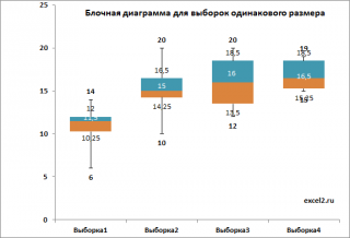
Из блочной диаграммы видно, что концентрация добавки влияет на
прочность нити
Y (чем выше концентрация, тем в среднем прочнее нить). Однако, мы пока не можем сделать статистически обоснованный вывод, о том что
концентрация добавки
влияет на
прочность нити
. Возможно, различие в
средних значениях
выборок обусловлено лишь случайностью выборок.
Примечание
: Из
блочной диаграммы
видно, что разброс данных (его отражает дисперсия выборки) имеет примерно одинаковую величину для всех 4-х выборок, что является обязательным условием для корректности применения метода
дисперсионного анализа
.
Сделаем вспомогательные вычисления по формулам из предыдущего раздела статьи: вычислим средние значения каждой выборки, общее среднее, суммы квадратов SS, степени свободы, MSE, MSA.
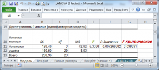
Тестовая статистика
вычисляется по формуле:
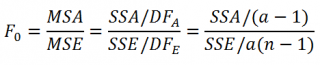
Т.к.
тестовая статистика
имеет
F
-распределение (
распределение Фишера
)
, то ее значение, вычисленное на основании наблюдений, должно лежать около
среднего значения
F
-распределения
с соответствующими
степенями свободы
.

В нашем случае среднее значение
F
-распределения
с
3
и
20
степенями свободы
равно 1,11. Если вычисленное нами значение F
0
«значительно» превосходит это значение, то это является маловероятным событием и у нас есть основания для отклонения
нулевой гипотезы
.
В нашей задаче F
0
равно 5,3358. «Значительно» это или нет? Для ответа на этот вопрос вычислим вероятность этого события (т.е. вероятность события, что случайная величина F, имеющая
распределение Фишера
с указанными степенями свободы, примет значение 5,3358 или более). Эта вероятность не высока =0,0072. Этого и следовало ожидать, т.к. 5,3358 значительно больше среднего значения 1,11. В MS EXCEL эту вероятность можно вычислить по формуле:
=
F.РАСП.ПХ((F
0
;a-1;a(n-1))=F.РАСП.ПХ((5,3358;3;20)
0,0072 – это так называемое
p
-значение
, т.е. вероятность, что статистика F
0
примет вычисленное значение.
Примечание
: Обычно под F
0
понимается как сама случайная величина —
тестовая статистика
F
0
, так и ее конкретное значение F
0
, вычисленное из условий задачи (исходных данных).
Теперь сравним
p
-значение
с
уровнем значимости
(обычно 0,05 или 0,01). Если
p
-значение
меньше
уровня значимости
, то нулевую гипотезу отклоняют.
В начале статьи мы задались вопросом о том, как математически точно определить «значимое» отличие
средних значений выборок
(чтобы мы могли сделать вывод, что уровни фактора влияют на значение переменной Y). Теперь мы можем утверждать, что
средние выборок
статистически значимо отличаются, если вычисленное
p
-значение
меньше заданного
уровня значимости
.
Таким образом, наша модель является полезной и наше предположение о зависимости Y (прочности нити) от фактора (концентрации добавки) является статистически обоснованным.
Примечание
: Однофакторный дисперсионный анализ можно также выполнить с помощью
надстройки Пакет анализа
. Об этом см.
в статье здесь
.