What is a x axis in excel

horizontal.
The horizontal (category) axis, also known as the x axis, of a chart displays text labels instead of numeric intervals and provides fewer scaling options than are available for a vertical (value) axis, also known as the y axis, of the chart.

What is the x-axis used for?

The line on a graph that runs horizontally (left-right) through zero. It is used as a reference line so you can measure from it.

Which column is x-axis in Excel?

Click “Edit” under the “Horizontal Axis Labels” list to open the “Axis Labels” dialog. Click the icon that displays a red arrow, and then highlight the column on the spreadsheet that you want to denote as the x-axis. In this example, this is all the numbers in column A.

What is an x-axis example?

X-axis is a horizontal axis. An example of an x-axis is the line across the bottom of a chart.The horizontal (H), or nearest horizontal, plane on a two- or three-dimensional grid, chart, or graph in a Cartesian coordinate system. See also Cartesian coordinates, y-axis, and z-axis.

How do you create an x-axis in Excel?

From the Design tab, Data group, select Select Data. In the dialog box under Horizontal (Category) Axis Labels, click Edit. In the Axis label range enter the cell references for the x-axis or use the mouse to select the range, click OK. Click OK.

What information is on x-axis?

The Axes. The independent variable belongs on the x-axis (horizontal line) of the graph and the dependent variable belongs on the y-axis (vertical line).

Is x-axis up or down?

The x-axis and y-axis are two lines that create the coordinate plane. The x-axis is a horizontal line and the y-axis is a vertical line.Reminder: the x-axis really runs left and right, and the y-axis runs up and down.

How do you find the x and y-axis?

Scientists like to say that the “independent” variable goes on the x-axis (the bottom, horizontal one) and the “dependent” variable goes on the y-axis (the left side, vertical one).

Do you say X or y-axis first?

The x-coordinate always comes first, followed by the y-coordinate.

What is the meaning of X coordinate?

Definition of x-coordinate
: a coordinate whose value is determined by measuring parallel to an x-axis specifically : abscissa.

What is the equation of x-axis?

The equation of the x-axis is x=0.

How do I move the X-axis in Excel?

Select the cluster column chart whose horizontal axis you will move, and click Kutools > Chart Tools > Move X-axis to Negative/Zero/Bottom.

How do you add X-axis labels in Excel?

Click the chart, and then click the Chart Layout tab. Under Labels, click Axis Titles, point to the axis that you want to add titles to, and then click the option that you want. Select the text in the Axis Title box, and then type an axis title.

How do I change the X-axis scale in Excel?

You can change the scale used by Excel by following these steps:

1. Right-click on the axis whose scale you want to change. Excel displays a Context menu for the axis.
2. Choose Format Axis from the Context menu.
3. Make sure the Scale tab is selected.
4. Adjust the scale settings, as desired.
5. Click on OK.

Where is the x-axis on a bar graph?

The vertical axis of the bar graph is called the y-axis, while the bottom of a bar graph is called the x-axis.

What does the x-axis represent on a graph?

the horizontal line of figures along the bottom of a graph, often representing time: The x-axis represents expenditure and the y-axis profit.

Where does the x-axis go?

An x-axis is one of the axes of a two- or three-dimensional graph. The x-axis is the horizontal plane of a graph in a Cartesian coordinate system, which gives a numerical value to each point along the horizontal x-axis, as well as the vertical y-axis (in a two-dimensional graph).

Is X vertical or horizontal?

A horizontal line is a line extending from left to right. When you look at the sunrise over the horizon you are seeing the sunrise over a horizontal line. The x-axis is an example of a horizontal line.

What is an X and Y coordinate?

The x coordinate is a given number of pixels along the horizontal axis of a display starting from the pixel (pixel 0) on the extreme left of the screen. The y coordinate is a given number of pixels along the vertical axis of a display starting from the pixel (pixel 0) at the top of the screen.

Tips to show, hide, and edit the three main axes in an Excel chart

Updated on January 27, 2021

What to Know

• Select a blank area of the chart to display the Chart Tools on the right side of the chart, then select Chart Elements (plus sign).
• To hide all axes, clear the Axes check box. To hide one or more axes, hover over Axes and select the arrow to see a list of axes.
• Clear the check boxes for the axes you want to hide. Select the check boxes for the axes you want to display.

This article explains how to display, hide, and edit the three main axes (X, Y, and Z) in an Excel chart. We’ll also explain more about chart axes in general. Instructions cover Excel 2019, 2016, 2013, 2010; Excel for Microsoft 365, and Excel for Mac.

Hide and Display Chart Axes

To hide one or more axes in an Excel chart:

1. Select a blank area of the chart to display the Chart Tools on the right side of the chart.

2. Select Chart Elements, the plus sign (+), to open the Chart Elements menu.

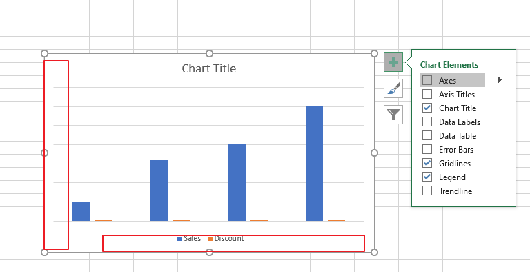
3. To hide all axes, clear the Axes check box.

4. To hide one or more axes, hover over Axes to display a right arrow.

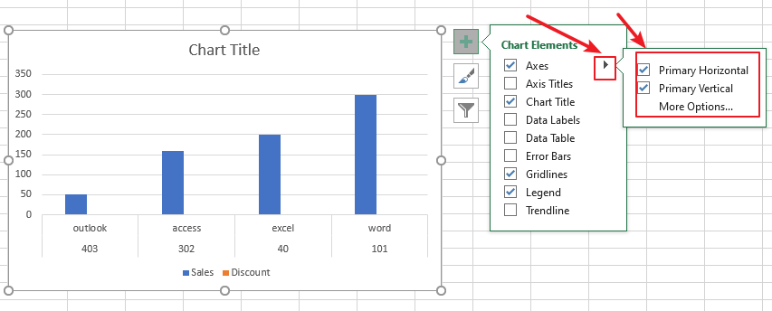
5. Select the arrow to display a list of axes that can be displayed or hidden on the chart.

6. Clear the check box for the axes you want to hide.

7. Select the check boxes for the axes you want to display.

What Is an Axis?

An axis on a chart or graph in Excel or Google Sheets is a horizontal or vertical line containing units of measure. The axes border the plot area of column charts, bar graphs, line graphs, and other charts. An axis displays units of measure and provides a frame of reference for the data displayed in the chart. Most charts, such as column and line charts, have two axes that are used to measure and categorize data:

The vertical axis: The Y or value axis.

The horizontal axis: The X or category axis.

All chart axes are identified by an axis title that includes the units displayed in the axis. Bubble, radar, and pie charts are some chart types that do not use axes to display data.

3-D Chart Axes

In addition to horizontal and vertical axes, 3-D charts have a third axis. The z-axis, also called the secondary vertical axis or depth axis, plots data along the third dimension (the depth) of a chart.

Vertical Axis

The vertical y-axis is located along the left side of the plot area. The scale for this axis is usually based on the data values that are plotted in the chart.

Horizontal Axis

The horizontal x-axis is found at the bottom of the plot area, and contains category headings taken from the data in the worksheet.

Secondary Vertical Axis

A second vertical axis, which is found on the right side of a chart, displays two or more types of data in a single chart. It is also used to chart data values.

A climate graph or climatograph is an example of a combination chart that uses a second vertical axis to display both temperature and precipitation data versus time in a single chart.

Thanks for letting us know!

Get the Latest Tech News Delivered Every Day

Subscribe

In this video, we’ll take a look at the axes you’ll find in Excel charts.

A chart axis works like a reference line or scale for data plotted in a chart.

Excel has two primary types of chart axes. The first type is called a value axis, which is used to plot numeric data. Often, the vertical axis in a chart is a value axis.

The other primary axis type is called a category axis, which often appears as a horizontal axis. A category axis is used to group dates or text.

When you hover your mouse over an axis in an Excel chart, Excel will display the axis name. The axis type will always appear in parentheses.

The number of axes you see in a chart varies by chart type. Pie charts, doughnut charts, sunburst charts, and treemap charts have no axes.

Excel’s standard two dimensional charts have two axes, as you can see in these examples of a bar chart, column chart, line chart, and area chart.

Many chart types allow a secondary vertical axis. In this example, a secondary vertical axis is used to plot net profit. So, in this case the chart has 3 axes.

Three dimensional charts in Excel have a third axis, the depth axis. The depth axis is also called a series axis or z axis. It allows data to be plotted along the depth of a chart.

Not all chart types display axes the same way. XY scatter charts and bubble charts show numeric values on both the horizontal axis and the vertical axis.

For example, this xy scatter chart shows how the cost of a backpacking tent generally decreases as weight increases.

In the chart, both of these items have numeric values, and the data points are plotted on the x and y axes relative to their numeric values.

In column, line, and area charts, you’ll see numeric values on the vertical axis and categories on the horizontal axis.

For example, in this column chart, the vertical axis is a value axis plotting sales, and the horizontal axis is a category axis plotting quarters.

In this line chart, the interest rate is plotted on the vertical axis, and time is plotted across the horizontal category axis.

Chart axes can be displayed or hidden using the Chart Elements menu. For example, I can hide and unhide the vertical axis in this chart using the checkbox.

Excel provides a lot of control over how axes are formatted and displayed.

We’ll cover these settings in more detail in upcoming videos.

Sometimes, when you create a chart in Excel, you may want to switch the axis in the chart (i.e., interchange the X and the Y-axis)

It’s really easy, and in this short tutorial, I will show you how you can switch axis in Excel charts with a few clicks.

So let’s get started!

Understanding Chart Axis in Excel Charts

If you create a chart (for example, a column or bar chart), you will get the X and Y-axis.

The X-axis is the horizontal axis, and the Y-axis is the vertical axis.

Axis has values (or labels) that are populated from the chart data.

Let’s now see how to create a scatter chart, which will further make it clear what an axis is in an Excel chart.

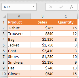
For creating a chart, I will be using the below data set, which contains products in column A, Sales value in column B, and Quantity value in column C.

In order to create a chart, you need to follow the below steps:

1. Select a range of values that you want to present on a chart (in this example B1:C10)
2. Go to the Insert tab
3. Select Insert Scatter chart icon
4. Choose the Scatter chart

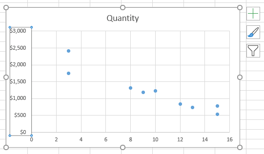
As a result, you get the scatter chart as shown below (where I have highlighted the axis using the arrow).

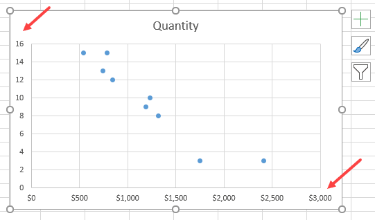
This chart has the X-axis (horizontal) with values from the Sales column and Y-axis (vertical) with values from the Quantity column.

When you create a chart in Excel, it automatically decides the range that needs to be shown on the axis.

Now that’s all good!

But what if I want a chart where Sales are on Y-Axis and Quantity on X-axis?

Thankfully, Excel allows you to easily switch the X and Y axis with a few clicks.

Let’s see how to do this!

Now, if you want to display Sales values on the Y-axis and Quantity values on X-axis, you need to switch the axis in the chart.

Below are the steps to do this:

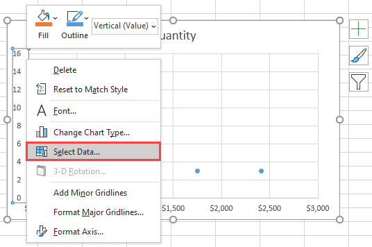
1. You need to right-click on one of the axes and choose Select Data. This way, you can also change the data source for the chart.

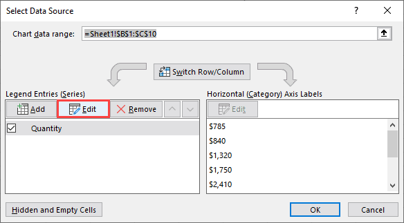
1. In the ‘Select Data Source’ dialog box, you can see vertical values (Series), which is X axis (Quantity). Also, on the right side, there are horizontal values (Category), which is the Y axis (Sales). You have to click on the Edit on the left side in order to switch axes.

1. In the pop-up window, you can see that Series X values are range “=Sheet1!$B$2:$B$10”, and the Series Y values are range “=Sheet1!$C$2:$C$10”.

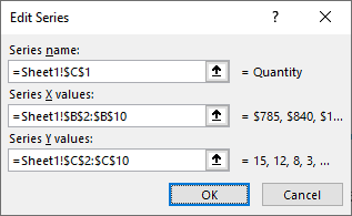
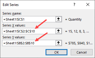
1. In order to switch values, you have to swap these two ranges, so that the range for series X becomes a range for series Y and vice versa. So, in Series X values, enter “=Sheet1!$C$2:$C$10”, and in Series Y values, enter “=Sheet1!$B$2:$B$10”.

1. After you confirm changes, you will be redirected back to the Select Data Source window and click OK.

Finally, your chart has a switched axis. As you can see, Sales values are now on the Y-axis, and Quantity values are on the X-axis.

Also read: How to Add Secondary Axis in Excel Charts?

Rearrange the Data to Specify the Axis

The above method works great when you have already created the chart, and you want to swap the axis.

But if you haven’t created the chart already, one way could be to rearrange the data so that Excel picks up the data and plots it on the X and Y axis as per your needs.

Excel, by default, sets the first column of the data source on the X-axis and the second column on the Y-axis.

In this case, you can just move Quantity in column B and Sales in column C.

Switching the axis option in a chart gives you more flexibility for adjusting the chart axis. Also, this way, you don’t need to change any data in your sheet.

So these are two simple and easy ways to switch the axis in Excel charts.

While I have shown an example of a scatter chart in this tutorial, you can use the same steps to switch axis in case of any chart in Excel.

I hope you found this Excel tutorial useful!

Other Excel tutorials you may also like:

• How to Move a Chart to a New Sheet in Excel
• How to Add Axis Titles in Excel?
• How to Insert an Excel file into MS Word (3 Easy Ways)
• How to Create Bar of Pie Chart in Excel?
• How to Insert Chart Title in Excel?
• How to Add Border to a Chart in Excel?
• How to Create a Waterfall Chart in Excel?
• How to Make Box Plot (Box and Whisker Chart) in Excel?

Excel has some useful chart types that can be used to plot data and show analysis.

A common scenario is where you want to plot X and Y values in a chart in Excel and show how the two values are related.

This can be done by using a Scatter chart in Excel.

For example, if you have the Height (X value) and Weight (Y Value) data for 20 students, you can plot this in a scatter chart and it will show you how the data is related.

Below is an example of a Scatter Plot in Excel (also called the XY Chart):

In this tutorial, I will show you how to make a scatter plot in Excel, the different types of scatter plots, and how to customize these charts.

What is a Scatter Chart and When To Use It?

Scatter charts are used to understand the correlation (relatedness) between two data variables.

A scatter plot has dots where each dot represents two values (X-axis value and Y-axis value) and based on these values these dots are positioned in the chart.

A real-life example of this could be the marketing expense and the revenue of a group of companies in a specific industry.

When we plot this data (Marketing Expense vs. Revenue) in a scatter chart, we can analyze how strongly or loosely these two variables are connected.

Creating a Scatter Plot in Excel

Suppose you have a dataset as shown below and you want to create a scatter plot using this data.

The aim of this chart is to see whether there is any correlation between the marketing budget and the revenue or not.

For making a scatter plot, it’s important to have both the values (of the two variables that you want to plot in the scatter chart) in two separate columns.

The column on the left (Marketing Expense column in our example) would be plotted on the X-Axis and the Revenue would be plotted on the Y-Axis.

Below are the steps to insert a scatter plot in Excel:

1. Select the columns that have the data (excluding column A)

1. Click the Insert option

1. In the Chart group, click on the Insert Scatter Chart icon

1. Click on the ‘Scatter chart’ option in the charts thats show up

The above steps would insert a scatter plot as shown below in the worksheet.

The column on the left (Marketing Expense column in our example) would be plotted on the X-Axis and the Revenue would be plotted on the Y-Axis. It’s best to have the independent metric in the left column and the one for which you need to find the correlation in the column on the right.

Adding a Trend Line to the Scatter Chart

While I will cover more ways to customize the scatter plot in Excel later in this tutorial, one thing that you can do immediately after building the scatter plot is to add a trend line.

It helps you quickly get a sense of whether the data is positively or negatively correlated, and how tightly/loosely correlated it is.

Below are the steps to add a trendline to a scatter chart in Excel:

1. Select the Scatter plot (where you want to add the trendline)
2. Click the Chart Design tab. This is a contextual tab which only appears when you select the chart

1. In the Chart Layouts group, click on the ‘Add Chart Element’ option

1. Go to the ‘Trendline’ option and then click on ‘Linear’

The above steps would add a linear trendline to your scatter chart.

Just by looking at the trendline and the data points plotted in the scatter chart, you can get a sense of whether the data is positively correlated, negatively correlated, or not correlated.

In our example, we see a positive slope in the trendline indicating that the data is positively correlated. This means that when the marketing expenses go up then the revenue goes up and if the marketing expenses go down then the revenue goes down.

In case the data is negatively correlated, then there would be an inverse relation. In that case, if the marketing expenses go up then the revenue would go down and vice versa.

And then there is a case where there is no correlation. In this case, when the marketing expenses increase, their revenue may or may not increase.

Note that the slope only tells us whether the data is positively or negatively correlated. it doesn’t tell us how closely it’s related.

For example, in our example, by looking at the trendline we cannot say how much the revenue will go up when the marketing expense increases by 100%. This is something that can be calculated using the correlation coefficient.

You can find that using the below formula:

=CORREL(B2:B11,C2:C11)

The correlation coefficient varies between -1 and 1, where 1 would indicate a perfectly positive correlation and -1 would indicate a perfectly negative correlation

In our example, it returns 0.945, indicating that these two variables have a high positive correlation.

Identifying Clusters using Scatter Chart (Practical Examples)

One of the ways I used to use scatter charts in my work as a financial analyst was to identify clusters of data points that exhibit a similar kind of behavior.

This usually works well when you have a diverse data set with less overall correlation.

Suppose you have a data set as shown below, where I have 20 companies with their revenue and profit margin numbers.

When I create a scatterplot for this data, I get something as shown below:

In this chart, you can see that the data points are all over the place and there is a very low correlation.

While this chart doesn’t tell us much, one way you can use it to identify clusters in the four quadrants in the chart.

For example, the data point in the bottom left quadrant are those companies where the revenue is low and the net profit margin is low, and the companies in the bottom right quadrant are those where the revenue is high but the net profit margin is low.

This used to be one of the highly discussed charts in the management meeting when we used to identify prospective customers based on their financial data.

Different Types of Scatter Plots in Excel

Apart from the regular scatter chart that I have covered above, you can also create the following scatter plot types in Excel:

• Scatter with Smooth Lines
• Scatter with Smooth Lines and Markers
• Scatter with Straight Lines
• Scatter with Straight Lines and Markers

All these four above scatter plots are suitable when you have fewer data points and when you’re plotting two series in the chart.

For example, suppose you have the Marketing Expense vs Revenue data as shown below and you want to plot a scatter with smooth lines chart.

Below are the steps to do this:

1. Select the dataset (excluding the company name column)
2. Click the Insert tab
3. In the Charts group, click on the Insert Scatter Chart option
4. Click on Scatter with Smooth Lines and Markers options

You will see something as shown below.

This chart can quickly become unreadable if you have more data points. This is why it is recommended to use this with fewer data points only.

I have never used this chart in my work as I don’t think it gives any meaningful insight (since we can’t plot more data points to it).

Customizing Scatter Chart in Excel

Just like any other chart in Excel, you can easily customize the scatter plot.

In this section, I will cover some of the customizations you can do with a scatter chart in Excel:

Adding / Removing Chart Elements

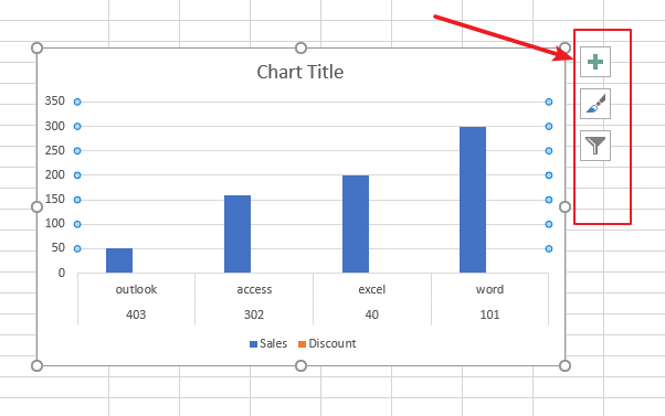
When you click on the scatter chart, you will see plus icon at the top right part of the chart.

When you click on this plus icon, it will show you options that you can easily add or remove from your scatter chart.

Here are the options that you get:

• Axes
• Axis Title
• Chart Title
• Data Labels
• Error Bars
• Gridlines
• Legend
• Trendlines

Some of these options are already present in your chart, and you can remove these elements by clicking on the checkbox next to the option (or add these by clicking the checkbox if not checked already).

For example, if I want to remove the Chart Title, I can simply uncheck the option and it would be gone,

In case you need more control, you can click on the little black arrow that appears when you hover the cursor hover over any of the options.

Clicking on it will give you more options for that specific chart element (these open as a pane on the right side).

Note: All the screenshots I have shown you are from a recent version of Excel (Microsoft 365). In case you’re using an older version, you can get the same options when you right-click on any of the chart elements and click on the Format option.

Let’s quickly go through these elements and some of the awesome customizations you can do to scatter charts using it.

Axes

Axes are the vertical and horizontal values that you see right next to the chart.

One of the most useful customizations you can do with axes is to adjust the maximum and minimum value it can show.

To change this, right-click on the axes in the chart and then click on Format axes. This will open the Format Axis pane.

In the Axis option, you can set the minimum and maximum bounds as well as the major and minor units.

In most cases, you can set this to automatic, and Excel will take care of it based on the dataset. But in case you want specific values, you can change them from here.

One example could be when you don’t want the minimum value in the Y-axis to be 0, but something else (say 1000). Changing the lower bound to 1000 will adjust the chart so that the minimum value in the vertical axis would then be 1000.

Axis Title

The Axis title is something you can use to specify what the X and Y-axis represent in the scatter chart in Excel.

In our example, it would be the Net Income for the X-axis and Marketing Expense for the Y-axis.

You can choose to not show any axis title, and you can remove these by selecting the chart, clicking on the plus icon, and then unchecking the box for Axis title.

To change the text in the axis title, simply double-click on it and then type whatever you want as the axis title.

You can also link the Axis title value to a cell.

For example, if you want the value in cell B1 to show up in the vertical axis title, click on the axis title box and then enter =B1 in the formula bar. This will show the value in cell B1 in the axis title.

You can do the same for the horizontal axis title and link it to a specific cell. This makes these titles dynamic and if the cell value changes, the axis titles will also change.

If you need more control on formatting the axis titles, click on any axis, right-click and then click on Format Axis Title.

With these options, you can change the fill and border of the title, change the text color, alignment, and rotation.

Chart Title

Just like Axis titles, you can also format the Chart title in a scatter plot in Excel.

A chart title is usually used to describe what the chart is about. For example, I can use ‘Marketing Expense Vs Revenue’ as the chart title.

If you don’t want the chart title, you can click and delete it. And in case you don’t have it, select the chart, click on the plus icon and then check the Chart Title option.

To edit the text in the Chart title, double-click on the box and manually type the text you want there. And in case you want to make the chart title Dynamic, you can click the title box and then type the cell reference or the formula in the formula bar.

To format the chart title, right-click on the Chart Title and then click on the ‘Format Chart Title’ option. This will show the Format Chart Title pane on the right.

With these options, you can change the fill and border of the title, change the text color, alignment, and rotation.

Data Labels

By default, data labels are not visible when you create a scatter plot in Excel.

But you can easily add and format these.

Do add the data labels to the scatter chart, select the chart, click on the plus icon on the right, and then check the data labels option.

This will add the data labels that will show the Y-axis value for each data point in the scatter graph.

To format the data labels, right-click on any of the data labels and then click on the ‘Format Data Labels’ option.

This will open the former data labels pane on the right, and you can customize these using various options listed in the pane.

Apart from the regular formatting such as fill, border, text color, and alignment, you also get some additional label options that you can use.

In the ‘Label Contains’ options, you can choose to show both the X-axis and the Y-axis value, instead of just the Y-axis.

You can also choose the option ‘Value from Cells’. which will allow you to have data labels that are there in a column in the worksheet (it opens a dialog box when you select this option and you can choose a range of cells whose values would be displayed in the data labels. In our example, I can use this to show company names in the data labels

You can also customize the position of the label and the format in which it’s shown.

Error Bars

While I have not seen error bars being used in scatter charts, Excel does have an option that allows you to add these error bars for each data point in the scatterplot in Excel.

To add the error bars, select the chart, click on the plus icon, and then check the Error Bars option.

And if you want to customize these error bars further, right-click on any of these error bars and then click on the ‘Format Error Bars’ option.

This will open the ‘Format Error Bars’ pane on the right, where you can customize things such as color, direction, and style of the error bars.

Gridlines

Gridlines are useful when you have a lot of data points on your chart as it allows the reader to quickly understand the position of the data point.

When you create a scatterplot in Excel, gridlines are enabled by default.

You can format these gridlines by right-clicking on any of the gridlines and clicking on the Format Gridlines option.

This will open the Format Gridlines pane on the right way you can change the formatting such as the color, thickness,  of the gridline.

Apart from the major gridlines that are already visible when you create the scatter diagram, you can also add minor gridlines.

Between two major gridlines, you can have a few minor gridlines that further improve the readability of the chart in case you have a lot of data points.

To add minor horizontal or vertical gridlines, select the chart, click the plus icon, and hover the cursor over the Gridlines option.

Click the thick black arrow there appears and then check the ‘Primary Minor Horizontal’ or ‘Primary Minor Vertical’ option to add the minor gridlines

Legend

If you have multiple series plotted in the scatter chart in Excel, you can use a legend that would denote what data point refers to what series.

By default, there is no legend when you create a scatter chart in Excel.

To add a legend to the scatter chart, select the chart, click the plus icon, and then check the legend option.

To format the legend, right-click on the legend that appears and then click on the ‘Format Legend’ option.

In the Format Legend pane that opens up, you can customize the fill color, border, and position of the legend in the chart.

Trendline

You can also add a trendline in the scatter chart that would show whether there is a positive or negative correlation in the data set.

I’ve already covered how to add a trendline to a scatter chart in Excel in one of the sections above.

3D Scatter Plot in Excel (are best avoided)

Unlike a Line chart, Column chart, or Area chart, there is no inbuilt 3D scatter chart in Excel.

While you can use third-party add-ins and tools to do this, I cannot think of any additional benefit that you will get with a 3D scatter chart as compared to a regular 2D scatter chart.

In fact, I recommend staying away from any kind of 3D chart as it has the potential of misrepresenting the data and portions in the chart.

So this is how you can create a scatter plot in Excel and customize it to make it fit your brand and requirements.

I hope you found this tutorial useful.

Other Excel tutorials you may also like:

• How to Spot Data Point in Excel Scatter Chart
• KPI Dashboard in Excel – Extract List of Companies from the Scatter Chart
• How to Make a PIE Chart in Excel
• How to Create an Area Chart in Excel
• How to Create Combination Charts in Excel
• Creating Actual vs Target Chart in Excel
• Calculate Area Under Curve in an Excel

This post will guide you how to show or hide chart Axis in your current worksheet in Excel 2013/2016. How do I show or hide Axes or 3-D chart Axes, Horizontal Axis, Vertical Axis or secondary Vertical Axis in your chart in Excel.

Normally, Once you create a newly chart based on your data in your worksheet, the vertical Axis and the horizontal Axis are displayed automatically in Excel. But for some cased, it is not necessary to display all or any of the axes for your specified chart. You can try to hide chart axis in Excel.

What is Axis in Excel

---

Each axis is a line on a chart that together define its structure and which the data plotted on the graph is measured against. The Y axis is the vertical access, in other words the one that goes up and down. The X access is horizontal and so it goes across a chart. The Y axis is sometimes known as the value axis. Having an axis is common on scatter diagrams or X-Y Charts, bar charts and others. You do not have one on a pie chart. Most of Chart types have two axes: vertical axis and horizontal axis.

In addition to vertical and horizontal axes, there is another axis called 3-D chart Axes, and also called the secondary vertical axis or depth axis, and it will plot data along the third dimension of a chart.

The secondary vertical axis shows the values for the associated data series, and it works well in a chart that show a combination of column and line charts.

Hide and Display Chart Axes

---

If you want to hide one or more axes in your excel chart in your current worksheet, and just do the following steps:

Step1: select a blank area of your chart, then the Chart Tools will be displayed on the right side of the chart.

Step2: select Chart Elements button on the Chart Tools, and click the plus sign(+), and the Chart Elements menu will appear.

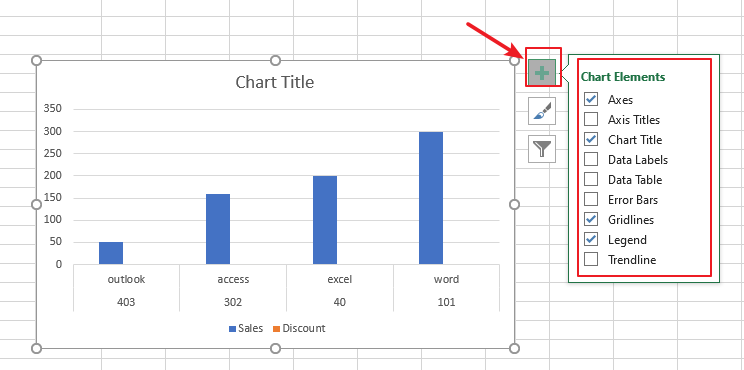
Step3: if you want to hide all chart axes, just uncheck the Axes check box.

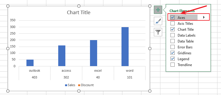
Step4: if you want to hide primary or secondary axis or more axes, and you need to click the right arrow to display a list of axes that can be hidden or displayed on the chart as you need. You just need to uncheck the check box for the axes that you want to hide.

Step5: To show one or more chart axes or one specified axis, and you just need to follow the above steps to check the check box for the axes that you want to display.